Characterizing Magnetohydrodynamic Turbulence in the Small Magellanic Cloud

Abstract

We investigate the nature and spatial variations of turbulence in the Small Magellanic Cloud (SMC) by applying several statistical methods on the neutral hydrogen (HI) column density image of the SMC and a database of isothermal numerical simulations. By using the 3rd and 4th statistical moments we derive the spatial distribution of the sonic Mach number (${\cal M}_{s}$) across the SMC. We find that about 90% of the HI in the SMC is subsonic or transonic. However, edges of the SMC ‘bar’ have ${\cal M}_{s}\sim 4$ and may be tracing shearing or turbulent flows. Using numerical simulations we also investigate how the slope of the spatial power spectrum depends on both sonic and Alfvén Mach numbers. This allows us to gauge the Alfvén Mach number of the SMC and conclude that its gas pressure dominates over the magnetic pressure. The super-Alfvénic nature of the HI gas in the SMC is also highlighted by the bispectrum, a three-point correlation function which characterizes the level of non-Gaussianity in wave modes. We find that the bispectrum of the SMC HI column density displays similar large-scale correlations as numerical simulations, however it has localized enhancements of correlations. In addition, we find a break in correlations at a scale of $\sim 160$ pc. This may be caused by numerous expanding shells of a similar size.

1. Introduction

In the recent decade, many advances in both observations and computational models have provided new insights into the workings and evolution of the interstellar medium (ISM). The emerging picture is that interstellar turbulence plays the key role in ISM structure formation and evolution (McKee & Ostriker 2007). In the Galaxy and the Magellanic Clouds, the ISM is turbulent on scales ranging from less than a parsec to a few kiloparsecs (Crovisier & Dickey 1983; Stanimirovic et al. 1999; Deshpande et al. 2000; Dickey et al. 2001; Elmegreen et al. 2001; Elmegreen & Scalo 2004). Although the observational evidence for the importance of turbulence in the ISM is overwhelming, many questions remain open. For example, what are the dominant energy sources and physical processes that convert kinetic energy into turbulence (Burkert 2006)? At what scales and through which modes is turbulent energy dissipated (Heyer & Zweibel 2004)? How do the level and type of turbulence depend on properties of the interstellar gas (e.g. presence/absence of star formation, presence/absence of tidal effects, or the strength of magnetic field)? Since no complete theory of astrophysical turbulence exists, studying its effects on the multiphase ISM can be challenging and calls for a combination of numerical and observational efforts.

Statistical studies have proved to be important in characterizing the magnetized turbulent ISM Lazarian (2009), however the interpretation of results is not always straight forward. Several statistical methods have been extensively used for both observational and synthetic data. These statistics include probability density functions (PDFs), wavelets, the principal component analysis, higher order moments, Velocity Coordinate Spectrum (VCS), and Velocity Channel Analysis (VCA), to name just a few (Gill & Henriksen 1990; Brunt & Heyer 2002; Kowal, Lazarian & Pogosyan 2000, 2004, 2006; Lazarian & Beresnyak 2007).

Most of these statistical methods require large datasets with a large spatial or velocity dynamic range, and produce a single, mostly one-dimensional, measure. This results in the lack of spatial information about turbulent properties across a given interstellar cloud, or a galaxy, making a connection with underlying physical properties highly difficult.

In this paper we explore a new method for obtaining spatial information about the level and nature of ISM turbulence on the neutral hydrogen (HI) observations of the Small Magellanic Cloud (SMC). The SMC, a dwarf irregular galaxy in the Local Group, has a highly gas rich ISM environment (see, Stanimirovic et al. 1999, henceforth known as SX99), and is an excellent candidate for ISM studies. Being nearby (60 kpc, Westerlund (1991)), the SMC is distant enough for all its objects to be treated as having roughly the same distance, unlike the Milky Way where distance determination is relatively uncertain.

The HI observations of the SMC, obtained using the Australia Telescope Compact Array (ATCA) and the Parkes telescope (SX99), have been used for several investigations, including the HI spatial power spectrum and the kinematic study of HI, which revealed the existence of many expanding shells of gas and three supergiant shells. The power law index of HI density and velocity distributions was derived in SX99 and Stanimirovic & Lazarian (2001), while the Genus statistic in Chepurnov et al. (2008) revealed spatial variations of HI morphology. Because the SX99 SMC data set is well studied, it is a perfect candidate to investigate new statistical methods. We can acquire new information, but also test and confirm past results, as well as validate the promise of these statistical tools for further use in other observational studies.

In this study, we investigate turbulent properties of the HI in the SMC by applying the higher order moments on the HI column density image. We then use a database of MHD simulations to bootstrap the spatial distribution of the sonic Mach number across the SMC. The crucial aspect of our approach is the confluence of observations and numerical simulations: only by combining the two we can retrieve the spatial variations of turbulent properties. This is the reason why we oscillate between observational and synthetic data in this paper. We also investigate whether and how interstellar shocks leave footprints on the HI gas by employing the bispectrum, a three point statistical measure, on the SMC HI column density image. Again, to interpret our results we apply the same statistics on the database of MHD simulated column density images.

In particular, the paper is organized as follows. We start with § 2 by providing a brief summary of previous work regarding the statistical methods used in our study. In § 3 we describe the SMC HI column density map and the database of numerical simulations of compressible MHD turbulence used for the comparison with observations. In § 4 we introduce higher order moments and their dependence on the sonic and Alfvenic Mach numbers. We then apply higher order moments on the SMC HI observations to derive an image of the sonic Mach number across the SMC, in § 5. We compare our results with an observational estimate of the sonic Mach number of the cold neutral medium (CNM) in the SMC, based on a comparison of the spin and kinetic temperature of HI absorption profiles, in § 6. In § 7 we show how the power-law slope of the spatial power spectrum depends on the sonic Mach number and use this to gauge the Alfvenic Mach number of the HI gas seen in emission. In § 8 we present an analysis of the bispectrum of the SMC, as well as a brief discussion of the noise and windowing effects. In § 9 we provide a discussion of our results, followed by our conclusions.

2. Background on statistical methods used in this study

2.1. Higher order statistical moments

Higher order statistical moments of density fluctuations have been studied extensively. For example, the variance of density fluctuations has been shown to increase with the sonic Mach number ${\cal M}_{s}$ Nordlund & Padoan (1999); Ostriker et al. (2001). Therefore, if turbulence is the dominant structuring mechanism, ${\cal M}_{s}$ can be estimated from the variance of density fluctuations. However, the observable that is the most easily available from observations for various ISM tracers is the column density. While this is a less direct measure of turbulence compared to velocity, a comparison between observations and simulations is the most straight forward in case of column densities.

Only very recently, Kowal et al. (2007), henceforth referred to as KLB, have investigated how variance, skewness and kurtosis, the 2nd, 3rd and 4th order moments respectively, depend on ${\cal M}_{s}$. They found strong correlations: as the sonic Mach number increases, so does the Gaussian asymmetry of the column density (and density) PDFs due to gas compression via shocks, resulting in the increase of variance, skewness and kurtosis. KLB used limited resolution models of 128³ in their study, while Burkhart et al. (2009), henceforth known as BFKL, saw the same trends using high resolution isothermal simulations. In both studies, the moments had little dependence on the Alfvén Mach number (${\cal M}_{A}$), or the line-of-sight (LOS) orientation used for integrating 3-D simulated data cubes. These studies are motivational, and imply that the sonic Mach number of turbulence in interstellar clouds could be characterized by variance, skewness and kurtosis of observed column density distributions.

2.2. Spatial power spectrum

The two-dimensional spatial power spectrum characterizes the energy distribution over spatial scales. SX99 found that the spatial power spectrum of individual HI velocity slices is well fit by a power-law, with an average slope of $\approx-3$. Stanimirovic & Lazarian (2001) showed that the power-law slope steepens when several channels are integrated together, and used this to estimate the density power-law slope of $-3.3$ and the velocity slope of $-3.4$. No obvious breaks or preferred scales were found over the range of 30 pc to 4 kpc. The density and velocity spectral slopes are similar, and in the case of incompressible MHD turbulence, density behaves as a passive scalar and thus scales in the same way as velocity (Monin & Yaglom(1967), Lithwick & Goldreich (2001), Cho & Lazarian 2003). However, the estimated slopes are slightly more shallow than the predictions for the Kolmogorov spectrum ($~{}k^{-11/3}$), which is expected for incompressible fluids with a weak magnetic field.

However, different types of turbulence are expected to have different spectral slopes.

For example, in incompressible fluids with a strong magnetic field, the spectrum is expected to be even steeper and scale as $~{}k^{-13/3}$ (Biskamp 2003).

When the medium is supersonic (as we will see later applies to parts of the SMC), these relations are no longer valid due to shocks forming highly asymmetric density structures. KLB demonstrated that the spectral slope of MHD turbulence becomes more shallow with increasing ${\cal M}_{s}$. This can be understood as shocks in supersonic turbulence create more small scale structure in density Beresnyak, Lazarian & Cho (2005). This behavior was found to be weakly dependent of the Alfvén Mach number.

2.3. Bispectrum

While the spatial power spectrum has long been applied on both observations and simulations, it essentially uses only the amplitude of the Fourier transform of the initial signal, while the phase information is totally ignored. The bispectrum, however, is a three point statistical measure which incorporates both the amplitude and phase of the correlation of signals in Fourier space. Because of this, it can be used to search for nonlinear wave-wave interactions and characterize how shocks affect turbulent properties of the ISM. The bispectrum has been used in cosmology and gravitational wave studies to detect departures from Gaussianity Fry (1998); Scoccimarro (2000); Liguori et al. (2006), and for the characterization of wave-wave interactions in laboratory plasmas Intrator et al. (1989); Tynan et al. (2001). The first application of the bispectrum on synthetic astrophysical MHD turbulence was in BFKL.

BFKL found a general correlation between the bispectrum of 2D column density and 3D density maps for simulated data cubes of 512³ resolution. Also, supersonic models showed a much greater degree of correlation between structures of different scales than subsonic models. While comparing models with the same sonic Mach number, models with a stronger magnetic field (i.e. sub-Alfvénic) showed enhanced correlations. These results are encouraging and suggest that the bispectrum can be also used to provide insight into the nature of the turbulence cascade.

3. Data: SMC and Numerical Simulations

3.1. HI Observations of the SMC

The small-scale HI structure of the SMC was observed with the ATCA, a radio interferometer, in a mosaicking mode (Staveley-Smith et al. 1997). Observations of the same area were obtained also with the 64-m Parkes telescope, in order to map the distribution of large-scale features. Both sets of observations were then combined (see SX99), resulting in the final HI data cube with angular resolution of 98^′′, velocity resolution of 1.65 km s^-1, and 1-$\sigma$ brightness temperature sensitivity of 1.3 K, to the continuous range of spatial scales between 30 pc and 4.4 kpc. The velocity range covered with these observations is 90-215 km s^-1. For details about the ATCA and Parkes observations, data processing, and data combination (short spacings correction) see Staveley-Smith et al. (1997) and SX99.

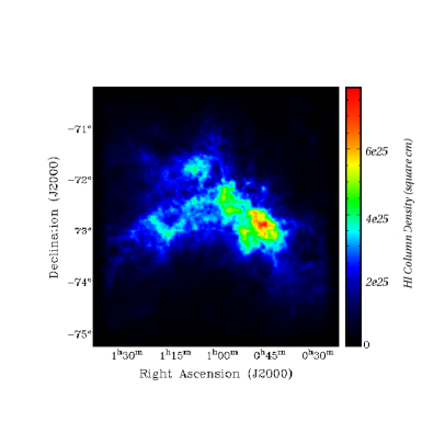
The HI column density image is shown in Figure  1. We corrected the original image by multiplying the HI column density of each pixel ($N_{HI}$ in atom cm^-2) with the correction factor $f_{c}$ derived by SX99:

$$f_{c}=\left\{\begin{array}[]{lr}1+0.667(\log N_{HI}-21.4)&:\log N_{HI}>21.4\\ 1&:\log N_{HI}\leq 21.4\end{array}\right.$$

Figure 1.— The final HI column density image after correction for self-absorption. The largest scale is $\sim 4.4$ kpc. The intensity range is in units of column density (cm^-2).

As the original Position-Position-Velocity (PPV) SMC cube has $578\times 610\times 78$ pixels, the resulting column density image is a 2D array with $578\times 610$ pixels.

3.2. A database of synthetic MHD cubes

We generate a database of 13 3D numerical simulations of isothermal compressible (MHD) turbulence by using the code of KLB and varying the input values for the sonic and Alfvénic Mach number. The sonic Mach number is defined as ${\cal M}_{s}\equiv\langle|{\bf v}|/C_{s}\rangle$, where is ${\bf v}$ is the local velocity, $C_{s}$ is the sound speed, and the averaging is done over the whole simulation. Similarly, the Alfvénic Mach number is ${\cal M}_{A}\equiv\langle|{\bf v}|/v_{A}\rangle$, where $v_{A}=|{\bf B}|/\sqrt{\rho}$ is the Alfvénic velocity, ${\bf B}$ is magnetic field and $\rho$ is density. KLB used resolution of 128³, while we use 512³. Details about KLB’s code were published (see Cho et al. 2003) and the code was used in several studies. We briefly outline the major points of their numerical setup.

The code is a second-order-accurate hybrid essentially nonoscillatory (ENO) scheme (see Cho & Lazarian, 2002) which solves the ideal MHD equations in a periodic box:

$$\frac{\partial\rho}{\partial t}+\nabla\cdot(\rho{\bf v})=0,$$ (1)

$$\frac{\partial\rho{\bf v}}{\partial t}+\nabla\cdot\left[\rho{\bf v}{\bf v}+\left(p+\frac{B^{2}}{8\pi}\right){\bf I}-\frac{1}{4\pi}{\bf B}{\bf B}\right]={\bf f},$$ (2)

$$\frac{\partial{\bf B}}{\partial t}-\nabla\times({\bf v}\times{\bf B})=0,$$ (3)

with zero-divergence condition $\nabla\cdot{\bf B}=0$, and an isothermal equation of state $p=C_{s}^{2}\rho$, where $p$ is the gas pressure. On the right-hand side, the source term $\bf{f}$ is a random large-scale driving force. We drive turbulence solenoidally, at wave scale $k$ equal to about 2.5 (2.5 times smaller than the size of the box). This scale defines the injection scale in our models in Fourier space to minimize the influence of the forcing on the generation of density structures. Density fluctuations are generated later on by the interaction of MHD waves. The time $t$ is in units of the large eddy turnover time ($\sim L/\delta V$) and the length in units of $L$, the scale of energy injection. The scale of energy dissipation is defined by the numerical diffusivity of the scheme. The magnetic field consists of the uniform background field and a fluctuating field: ${\bf B}={\bf B}_{\mathrm{ext}}+{\bf b}$. Initially ${\bf b}=0$.

We divided our models into two groups corresponding to sub-Alfvénic ($B_{\mathrm{ext}}=1.0$) and super-Alfvénic ($B_{\mathrm{ext}}=0.1$) turbulence. For each group we computed several models with different values of gas pressure (see Table 1). We ran compressible MHD turbulent models, with 512³ resolution, for $t\sim 5$ crossing times, to guarantee full development of energy cascade. Since the saturation level is similar for all models and we solve the isothermal MHD equations, the sonic Mach number is fully determined by the value of the isothermal sound speed, which is our control parameter. The models are listed and described in Table 1.

Table 1Description of the simulations - MHD, 512³

Model	$p_{gas}$	$B_{\rm ext}$	${\cal M}_{s}$	${\cal M}_{A}$	Description
1	2.00	1.00	0.1	0.7	subsonic & sub-Alfvénic
2	1.00	1.00	0.7	0.7	subsonic & sub-Alfvénic
3	0.10	1.00	2.0	0.7	supersonic & sub-Alfvénic
4	0.025	1.00	4.4	0.7	supersonic & sub-Alfvénic
5	0.01	1.00	7.0	0.7	supersonic & sub-Alfvénic
6	0.0077	1.00	8.4	0.7	supersonic & sub-Alfvénic
7	0.0049	1.00	10	0.7	supersonic & sub-Alfvénic
8	1.00	0.10	0.7	2.0	subsonic & super-Alfvénic
9	0.10	0.10	2.0	2.0	supersonic & super-Alfvénic
10	0.025	0.10	4.4	2.0	supersonic & super-Alfvénic
11	0.01	0.10	7.0	2.0	supersonic & super-Alfvénic
12	0.0077	0.10	8.4	2.0	supersonic & super-Alfvénic
13	0.0049	0.10	10	2.0	supersonic & super-Alfvénic

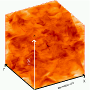
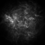
For each model, the results of MHD simulations are: the isothermal 3D density field, three components of velocity ($V_{x}$, $V_{y}$, $V_{z}$), and three components of magnetic field. As an example, Figure 2 (left) shows a density field for a sub-Alfvénic, subsonic simulation. To calculate the column density distribution we integrate the 3D density fields along a given LOS. We introduce the following nomenclature throughout the paper: “x column density” or “column density in the x direction” refers to the density cube being integrated along the x direction (parallel to the mean magnetic field). This description is similar for the y and z directions (perpendicular to $B_{ext}$). In the case of the Figure 2 (left), the LOS is along the z axis, and the magnetic field is oriented along the x axis.

Figure 2.— Left: An example of a simulated subsonic, sub-Alfv́enic (${\cal M}_{s}=0.7$, ${\cal M}_{A}=0.7$) $512^{3}$ density data cube demonstrating one possible direction of the LOS used to calculate the column density distribution. The mean magnetic field is oriented along the x direction. Here the LOS is along the z axis, although throughout the paper we integrate density fields along all three axes. Right: A supersonic column density image of a simulation with cloud boundaries, with a boundary radius similar (in pixel size) to what is seen for the SMC.

3.2.1 Scaling of the column density

In order to compare simulations with the SMC data, we apply a simple scaling to the simulated column density distributions:

$$N_{norm}=\frac{N-\langle N\rangle}{\sigma(N)},$$ (4)

where $\sigma(N)$ denotes the standard deviation and $\langle N\rangle$ denotes the arithmetic mean of the column density image. This method, often referred to as the standard score, standardizes all data sets used in this study. After the scaling, the new data set has values which represent the difference between the original data values and the sample mean, in units of the standard deviation. The same scaling was applied on the SMC HI column density image.

3.2.2 Simulating cloud boundaries

Another consideration to take into account is the fact that simulated cubes are periodic and do not have boundaries. In other words, simulations do not have a decrease in the column density values that is seen in the SMC data as one goes radially out from the center of the image. KLB showed that boundaries affect higher statistical moments of density, but have little effect on the spatial power spectrum and the bispectrum, generally only impacting the large scales.

To introduce cloud boundaries to our simulations, we multiply the simulated 3D density fields by a 3D spherical function, which has a value of one within a sphere of radius $R$ and is decaying outside of this radius with a Gaussian profile. We choose a $R$ value of 128 pixels, which is 4 times smaller then the box size. An example of the simulation with a boundary is shown in the right-hand panel in Figure 2. Please note that we impose cloud boundaries on the simulated cubes of homogeneous turbulence after turbulence has been fully developed. This results in the simulated column density profiles being similar to the SMC profile, however, is different from simulations of turbulence being developed within cloud boundaries.

4. Higher Order Moments: Simulated data

The most straightforward statistical properties of a distribution are the mean value and the variance. The mean arithmetic value and the variance of the distribution of, for example, column density $\xi$ are given by:

$$\bar{\xi}=\frac{1}{N}\sum_{i}^{N}\xi_{i}$$ (5)

and

$$\sigma_{\xi}^{2}=\frac{1}{N-1}\sum_{i}^{N}(\xi_{i}-\bar{\xi})^{2}$$ (6)

where $N$ is the number of samples or points of the mesh in the case of simulation data. The mean value is a less important property in our studies so we do not consider it here; however, it is required to calculate higher moments. Variance measures the width of the distribution and is always positby the third and fourth-order statistical moment. Skewness is defined as:

$$\gamma_{\xi}=\frac{1}{N}\sum_{i=1}^{N}{\left(\frac{\xi_{i}-\overline{\xi}}{\sigma_{\xi}}\right)^{3}}.$$ (7)

If a distribution $\xi$ is Gaussian, its skewness is zero. Negative skewness indicates the data are skewed in the left direction (the tail of the PDF is extended to the left, or towards low density values), while positive values imply that the distribution is skewed in the right direction (the tail of the PDF is extended to the right, or towards high density values).

Kurtosis is a measure of whether a quantity has a distribution that is peaked or flattened compared to a Gaussian distribution. Kurtosis is defined in a similar manner to skewness, only is derived from the forth order statistical moment. If a data set has positive kurtosis then the PDF of data values will have a distinct sharp peak near the mean and elongated tails. If a data set has a negative kurtosis then its PDF will be flat at the mean. Kurtosis is defined as:

$$\beta_{\xi}=\frac{1}{N}\sum_{i=1}^{N}\left(\frac{\xi_{i}-\overline{\xi}}{\sigma_{\xi}}\right)^{4}-3.$$ (8)

Figure 3.— Variation of the variance (left), skewness (middle), and kurtosis (right) with the sonic Mach number derived from the final snapshot of each simulation with cloud boundaries applied. For all simulations ${\cal M}_{A}$=0.7. Plotted data points are averages from data sets integrated along different LOS, with error bars representing the standard deviation between column density images with different LOS. As skewness and kurtosis increase almost linearly with ${\cal M}_{s}$, a linear function was fit over the range ${\cal M}_{s}\sim 1-8$ and is shown with a dashed-line. The measured skewness and kurtosis of the SMC HI column density image are: skewness$=1.52\pm 0.01$ and kurtosis$=2.45\pm 0.02$. Both of these values suggest that the HI in the SMC is supersonic, with a sonic Mach number $\geq 3$ within the error bars. This is discussed in Section 5.

Variance, skewness and kurtosis of simulated column densities depend on turbulent properties, specifically the sonic Mach number. This is shown in Figure 3 for the simulated column density distributions with cloud boundaries. Error bars are computed by estimating the standard deviation between models with the same sonic Mach number but differing LOS orientations. All three moments depend almost linearly on the sonic Mach number, for ${\cal M}_{s}\mathrel{\hbox{\hbox to0.0pt{\hbox{\lower 4.0pt\hbox{$\sim$}}\hss}\hbox{$>$}}}1-2$. KLB noticed a similar trend for supersonic simulations but focused only on ${\cal M}_{s}=0.2-2$. Our simulations extend this result all the way to ${\cal M}_{s}=8$. For ${\cal M}_{s}\mathrel{\hbox{\hbox to0.0pt{\hbox{\lower 4.0pt\hbox{$\sim$}}\hss}\hbox{$<$}}}0.5$ KLB found that both skewness and kurtosis have a rather flat dependence on the sonic Mach number, while the variance continues to decreases gradually for subsonic models. The increase of higher order moments with ${\cal M}_{s}$ can be explained in that as the Mach number increases, the abundance of small-scale density structure increases, resulting in a broader density PDF. BFKL showed that the increase of higher-order moments with ${\cal M}_{s}$ is not a resolution effect, since they replicated the result of KLB, (who used cubes of 128³ resolution) with cubes of 512³ resolution.

Which one of three high-order moments represents the best statistics to describe turbulence in observational data? While variance has a linear dependence over a broad range of ${\cal M}_{s}$ values, it depends on the exact scaling of the data set, making a direct comparison between simulations and observations difficult. On the other hand, skewness and kurtosis are, by definition, normalized by the standard deviation and do not have this problem. In addition, variance changes with the length along the LOS, since perturbations can add up in a random walk fashion. All of this, as well as the result by KLB that kurtosis is the least affected by cloud boundaries, suggest that for our immediate comparison of observations with the MHD simulations, the higher order moments, skewness and kurtosis, are more appropriate statistics.

4.1. Spatial Distribution of Skewness and Kurtosis

While it is useful to know the Mach number of the ISM in a global sense, even more interesting is to see how it varies spatially and whether it correlates with local star forming regions where high turbulence is expected. To characterize small scale departures from Gaussian distributions within the column density distributions, we create moment maps of the simulated column densities using a circular moving kernel. We do this by moving a circle of a given radius $r$ across the image and calculating the skewness and kurtosis at all points.

Figure 4.— The standard error in skewness (SES) and kurtosis (SEK) vs. radius of the circular kernel (related to the number of points or pixels within the kernel used to calculate the skewness/kurtosis). SES$=\sqrt{6/N}=\sqrt{\frac{6}{\pi r^{2}}}$, while SEK$=\sqrt{24/N}=\sqrt{\frac{24}{\pi r^{2}}}$. We choose $r=35$ pixels to retain good resolution and low SEK/SES. These error measurement describes how large the statistics must be before they are deemed significant deviations from Gaussianity. If statistics are in this range then they are deemed generally Gaussian. If statistics are outside of this range then departures from Gaussianity have occurred.

First we must decide on a kernel size that will enclose enough pixels to provide reliable statistics. According to Tabachnick & Fidell (1996), the standard error in skewness (SES) can be estimated by $\sqrt{6/N}$ and the standard error in kurtosis (SEK) can be estimated by $\sqrt{24/N}$, where $N$ is the number of points used to calculate the skewness/kurtosis. Generally, if a value of skewness/kurtosis falls within $\pm 2\times$SES/SEK, then the distribution is considered to be normal, while values of skewness/kurtosis larger than twice the absolute value of SES/SEK imply significant non-Gaussianity. Figure  4 shows $2\times$ SES and SEK as a function of the kernel radius $r$. Clearly, SES/SEK is proportional to $1/r$; the smaller the radius, the higher the absolute value of SES/SEK. Thus, we select $r=35$ pixels, which corresponds to the point where $2\times$ SES/SEK starts to deviate from zero and ensures that Gaussianity is represented by $2\times$ SES/SEK$\sim 0$.

Using a circular moving kernel we generate 3rd and 4th moment maps of simulated column density distributions. To ensure there are no resolution artifacts, we briefly explore correlations between skewness and kurtosis of the derived moment maps on a pixel-to-pixel basis. Based on the work by KLB and BFKL, and also our Figure 3, we expect for supersonic models a correlation of both skewness and kurtosis with the sonic Mach number, and that skewness and kurtosis agree in sign and relative value. However, as subsonic models show unexpected behavior at low resolutions (from the KLB study), the dependence of skewness and kurtosis on the sonic Mach number is not strong.

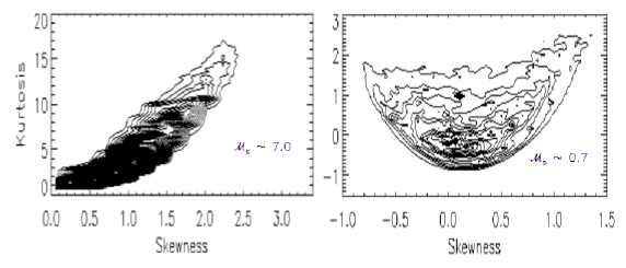
Figure 5 shows pixel-to-pixel comparison between skewness and kurtosis for two example models: a supersonic with ${\cal M}_{s}=7.0$ (left panel) and a subsonic with ${\cal M}_{s}=0.7$ (right panels). It is evident that the supersonic model shows a good correlation between kurtosis and skewness, while the subsonic model does not. This is exactly as expected. This result proves that our approach of deriving moment maps is not resolution limited although we use a smaller number statistics within each circular kernel ($\pi r^{2}=1380$ pixels). This also highlights another interesting property: regions of moment maps with a good correlation between skewness and kurtosis could be interpreted by supersonic MHD turbulence, while a poor correlation may be caused by subsonic turbulence. We present in the appendix another technique that could be used to further identify subsonic regions.

Figure 5.— Kurtosis vs. Skewness for isothermal simulations with a kernel of $r=35$ pixels. The left is a supersonic model, while the right is a subsonic model. The supersonic model shows good correlation between skewness and kurtosis while the subsonic model does not.

5. Higher order moments: the SMC HI column density image

We first calculate the higher order moments of the whole SMC HI column density image. We find that the skewness is 1.52$\pm 0.01$, and the kurtosis is $2.45\pm 0.02$. The estimated uncertainties are determined by calculating twice the SES or SEK. Figure 3 suggests that on average the HI in the SMC is supersonic with ${\cal M}_{s}\mathrel{\hbox{\hbox to0.0pt{\hbox{\lower 4.0pt\hbox{$\sim$}}\hss}\hbox{$>$}}}3$.

To characterize small scale departures from the Gaussian distribution within the SMC we create 3rd and 4th moment maps of the SMC using a circular kernel, as discussed for simulations in Section 4.1. We repeat a similar process for the SMC as we did with the simulations. We use a radius of $r=35$ and calculate moments in a circular kernel moving across the SMC. This is equivalent to convolving the original HI image with a Gaussian function with a FWHM of 30^′. The resultant moment images therefore have a lower resolution than the original HI image. After this we create a mask which cuts off pixels below a column density of $1.26\times 10^{21}$ cm^-2 in the HI column density image, to exclude increase in noise along the edges of the image. This is done to eliminate noisy pixels in moment maps, since pixels along the edge have significantly smaller column density values.

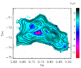
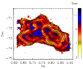
Figures 6 shows the distribution of skewness and kurtosis across the SMC (the HI column density image was standardized using the standard score method), with overlaid HI contours smoothed to 30^′ resolution. These maps retain the overall shape of the SMC, which can be seen in the HI contours. Familiar features of the SMC, such as the east wing and bar, regions of high star formation, can be picked out in these maps.

Figure 6.— (Left) Skewness of the HI column density derived using a circular kernel with $r=35$ pixels. HI contours are overlaid. (Right) Kurtosis of the HI column density with the HI contours overlaid. The contours show the HI column density and range from 20 to 90%, with a step of 15%.

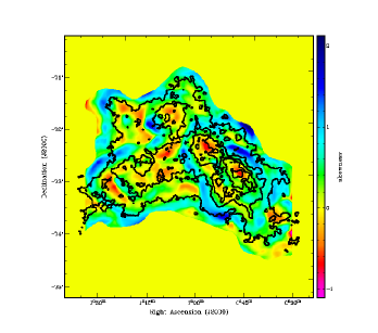
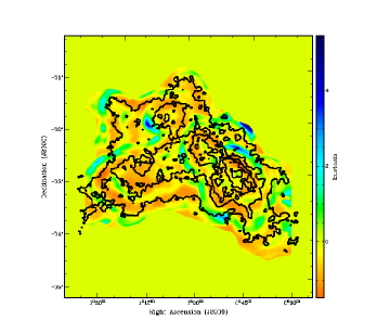
Generally, skewness ranges from $-0.5$ to 1, with several discrete regions reaching higher positive or negative values. For kurtosis, most pixels range from $-1$ to 1, with again several exceptions. Based on Figure 3, this suggest that large areas in the SMC have ${\cal M}_{s}=0-2$ and are subsonic or transonic. Along most of the bar the skewness and kurtosis correlate well. This suggests that the MHD turbulence could be the cause of local departures from Gaussianity in the HI column density distribution. We warn once again that both our study and earlier work find strong dependence of skewness and kurtosis on the sonic Mach number only for supersonic models, while the dependence for subsonic models is rather weak. Interpreting subsonic turbulence is therefore difficult, and poor correlation between skewness and kurtosis could be due to either subsonic turbulence or some other physical mechanisms. Several interesting regions stand out in Figure 6.

• Along the HI bar and the Eastern Wing region both skewness and kurtosis are negative, reaching values even lower than what is seen in Figure 3 for global averages. Based on expectations from numerical simulations this could be explained by the subsonic isothermal MHD turbulence, as shown in Figure 5. Most of the HI bar and the Wing therefore could be explained as being subsonic, with several discrete concentrations with almost no turbulence, probably tracing quiescent regions and potential sites of future star formation. However, as subsonic regions are hard to constrain from simulations, additional processes may be also playing an important role.

• From HI peaks radially outward, both skewness and kurtosis gradually increase. The highest values of both skewness ($\sim 2$) and kurtosis ($\sim 3-4$) are found along the HI bar and correspond to areas of compressed HI contours. These regions could be interpreted as having the highest level of turbulence (with ${\cal M}_{s}=\sim 4$) in the SMC. This suggests that the most turbulent regions may be associated with the shearing flows and/or shocks between the bar and the surrounding HI.

• Sudden change in the behavior of both skewness and kurtosis can be noticed around RA 01^h 10^m, Dec $-72^{\circ}$ 10^′. For example, skewness flips from high positive to high negative values over an angular scale of $\sim 60^{\prime}$. Interestingly, this flip happens in the direction of an HI extension towards the LMC and again may be pointing out streaming or tidal motions caused by the interactions between the SMC and the LMC.

Figure 7.— Histograms of the skewness and kurtosis maps from the simulations and the SMC HI column density image (see Figure 6), derived using the moving circle kernel with $r=35$. The top row shows kurtosis, and the bottom row shows skewness. The SMC distributions are overplotted with dashed lines and agree best within the ${\cal M}_{s}=2.0$ simulations.

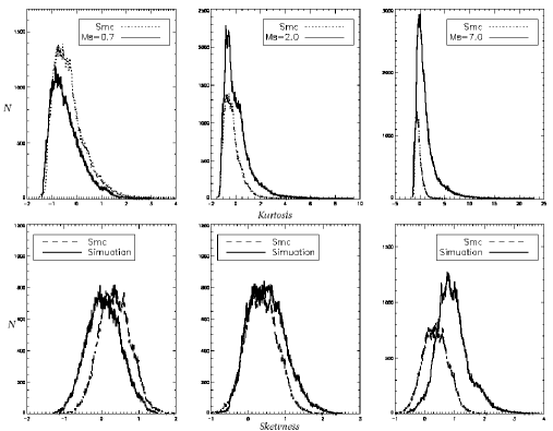
In order to compare the range of values found in the SMC and the simulations we plot several histogram of the skewness and kurtosis values in Figure 7. These figures show that the majority of SMC pixels generally match well with the mildly supersonic models with ${\cal M}_{s}\sim 1-2$. However, the SMC distribution appears to be more narrow in terms of both skewness and kurtosis values than the ${\cal M}_{s}\sim 2$ simulation. For subsonic and very supersonic models, the values of skewness and kurtosis of the SMC are not in the range of the simulations.

Figure 8.— (Left) The sonic Mach number image derived from the HI column density image of the SMC overlaid with the HI column density contours. The circle in the bottom-left shows the angular resolution of the image. (Right) Same as on the left but overlaid with the H$\alpha$ contours smoothed to the same resolution. The H$\alpha$ image is from Kennicutt et al. (1995).

5.1. The ${\cal M}_{s}$ map of the SMC

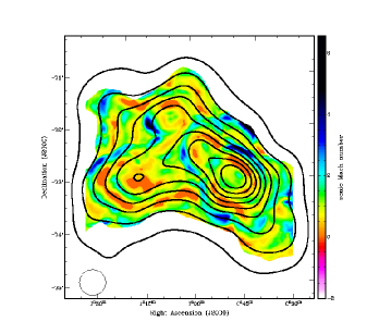
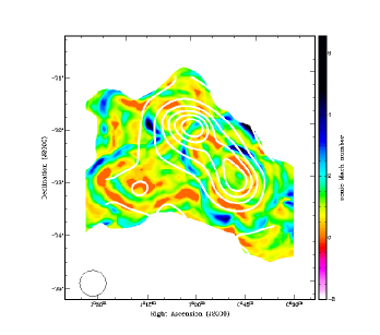
As shown above, with our limited angular resolution of 30^′ we see strong hints that different regions in the SMC have different turbulent properties, suggesting spatial variations of ${\cal M}_{s}$. We would now like to combine all this information into an image of ${\cal M}_{s}$ for the SMC. As already discussed, based on the KLB study, kurtosis is the least prone to effects caused by cloud boundaries and as Figure 3 suggests has an almost linear shape for ${\cal M}_{s}\sim 1-8$. Therefore, we fit a linear function for all values of kurtosis $>\sim-1$. This function can be inverted to estimate ${\cal M}_{s}$: ${\cal M}_{s}\sim({\rm kurtosis}+1.44)/1.05$. Pixels in the ${\cal M}_{s}$ image with corresponding kurtosis $<-1$ are set to zero and most likely mark subsonic regions, or could be caused by additional processes. The resultant map is shown in Figure 8 (left).

As expected already, most of the area of the SMC bar and the Eastern Wing could be interpreted as having subsonic or transonic Mach numbers, ${\cal M}_{s}\sim 0-2$. Several concentrated regions across the SMC indicate very quiescent environments, most of them unfortunately have a size close to our angular resolution. Regions with the highest sonic Mach number, ${\cal M}_{s}\sim 4$, are found around the bar and correspond to compressed HI contours.

We can quantify the fraction of HI with different ${\cal M}_{s}$. The most likely quiescent regions (set to zero in our map) comprise 8% of the mapped area. Regions with $0<{\cal M}_{s}\leq 1$ comprise about 40%, while about the same fraction is contained in transonic regions with ${\cal M}_{s}=1-2$. Regions with higher turbulence, ${\cal M}_{s}>2$ constitute about 10% of the area.

Figure 8 (right) shows contours of the H$\alpha$ emission (obtained by Kennicutt et al. 1995) smoothed to 30^′ and overlaid on the ${\cal M}_{s}$ map. Sites of the most recent star formation in the bar and the Eastern Wing have ${\cal M}_{s}\sim 1$, suggesting that the most turbulent regions are not associated with star formation. The most turbulent regions appear to trace shearing and tidal motions. We note though that our resolution of 30^′ is too low to trace individual star-forming regions.

As an estimate of the velocity dispersion along the LOS is often used as a possible measure of HI turbulence, we investigated how the HI velocity dispersion compares to our ${\cal M}_{s}$ map. Stanimirovic et al. (2004) found that regions with the highest dispersion ($\sim 30$ km s^-1) appear to be associated with the positions of the three largest super-giant shells. We find no obvious correlation between the HI velocity dispersion and our ${\cal M}_{s}$ map.

This lack of correlation could be due to projection effects, and/or large LOS depth of the SMC. In addition, velocity dispersion (similar to velocity centroids) is subject to the interplay of several statistical effects (Lazarian & Esquivel 2003, Esquivel & Lazarian 2005, Esquivel et al. 2007). The most obvious is the contribution of both velocities and densities to the resulting measure. More subtle, but still important, are effects of velocity-density correlations and non-Gaussianity. These effects make centroids unreliable when dealing with supersonic turbulence (Esquivel et al. (2007). Effects of phase transitions resulting in the existence of cold and warm HI and the pliable equation of state corresponding to interstellar HI are likely to act in a similar way. Thus the velocity dispersions obtained from spectral lines are substantially affected by densities, which are the quantities that we deal in this study. They should be distinguished from the true velocity dispersions, which, unfortunately, are not available through spectral line observations.

6. Comparison with the observationally inferred ${\cal M}_{s}$ of the CNM

Constraining the sonic Mach number of the warm neutral medium (WNM) observationally is highly difficult due to the lack of direct measurements of the HI temperature. This is the main reason why in the previous section we used the HI column density image of the SMC and a database of numerical simulations to explore spatial variations of ${\cal M}_{s}$. To investigate reliability of our results we compare our derived ${\cal M}_{s}$ distribution with results from an observational method which constrains temperature of the cold HI, and therefore ${\cal M}_{s}$ of the CNM. This method is based on the comparison of the spin temperature ($T_{s}$) with the upper limit on the kinetic temperature ($T_{k,max}$) for CNM clouds seen in HI absorption.

For observational data we use HI absorption and emission observations of 29 radio continuum sources behind the SMC by Dickey et al. (2000). For each of the sources Dickey et al. (2000) provided the FWHM linewidth of the absorption spectra, and estimated the spin temperature of the CNM seen in absorption. By assuming Doppler broadening of HI velocity profiles, we can estimate the upper limit on the kinetic temperature as $T_{k,max}=(FWHM/0.215)^{2}$. As shown in Heiles & Troland (2003), the ratio of $T_{k,max}$ and the spin temperature, $T_{s}$, is related to the 1D mean square turbulent velocity:

$$V_{t,1D}^{2}=\frac{kT_{s}}{m_{H}}\left(\frac{T_{k,max}}{T_{s}}-1\right),$$ (9)

where $k$ is the Boltzmann constant and $m_{H}$ is the mass of the hydrogen atom. Multiplying this by 3 gives the mean square 3D turbulence velocity $V_{t,3D}^{2}$ of the CNM. To estimate the sonic Mach number we need to divide $V_{t,3D}$ by the sound speed $C_{s}=\sqrt{kT_{s}/\mu m_{H}}$. We adopt a mean atomic weight of $\mu=1.22$ for the ISM of SMC abundance (see Mao et al. 2008). Using this, we can write:

$${{\cal M}_{s}}^{2}=\frac{{V_{t,3D}}^{2}}{{C_{s}}^{2}}=3.7\left(\frac{T_{k,max}}{T_{s}}-1\right).$$ (10)

For each of 29 radio continuum sources from Dickey et al. (2000) we derive $T_{k,max}$ and use the estimated $T_{s}$ to calculate the sonic Mach number of the CNM clouds. Dickey et al. (2000) used three different methods to estimate the spin temperature. As our aim is to compare ${\cal M}_{s}$ with values derived from the LOS integrated HI emission profiles, we use their LOS averaged spin temperature (or $T_{\rm ew}$). The median value of the spin temperature is 43 K.

A histogram of derived ${\cal M}_{s}$ values is shown in Figure 9. The median Mach number for the whole sample of 29 sources is ${\cal M}_{s}=4.7$, and the histogram peaks around ${\cal M}_{s}=3.5-4$. This suggests that the internal CNM macroscopic motions are highly supersonic. To compare these values with the ones derived using the method of higher-order statistical moments we show a histogram of data points from the ${\cal M}_{s}$ map in the right panel of Figure 9. While the observed histogram suffers from the low number statistics, due to a small number of suitable (strong) sources, the two histograms have a similar shape: almost a Gaussian central distribution with a tail at higher Mach values. Obviously, the observationally inferred ${\cal M}_{s}$ values suggest at least a factor of 2 higher level of turbulence across the SMC than what we derived using higher statistical moments. This is not surprising as the observed values trace predominately the CNM, while the ${\cal M}_{s}$ map was derived using the HI column density image and therefore is affected by both CNM and WNM. We discuss this further in §  9. In any case, to sample better CNM turbulence across the SMC future sensitive HI absorption observations of continuum sources behind the SMC are clearly needed.

Figure 9.— (Left) Histogram of the sonic Mach number of the CNM clouds in the SMC derived from the ratio $T_{s}/T_{k,max}$ using the HI absorption profiles against radio continuum sources. (Right) Histogram of the sonic Mach number from the ${\cal M}_{s}$ map derived using the higher statistical moments (see Figure 8).

7. Spatial Power Spectrum of Column Density

The slope of the Fourier transform of the two point autocorrelation function, or the spatial power spectrum, also provides information on important properties of turbulence flows. In particular, the slope of the power spectrum is known to depend on the sonic Mach number. With a database of numerical simulations we explore whether the slope of the spatial power spectrum depends also on the Alfvén Mach number. The Alfvén Mach number dependence would be especially interesting as we could use higher-order statistical moments to estimate the sonic Mach number, and from there the Alfvén Mach number and the strength of the magnetic field.

The power spectrum is defined as:

$$P(k)=\sum_{|\vec{k}=k|}{A(\vec{k})\cdot{A}^{*}(\vec{k}})$$ (11)

where $k$ is the wavenumber and $A(\vec{k})$ is the Fourier transform. Stanimirovic & Lazarian (2001) estimated the power-law slope of $-3.3$ for the spatial power spectrum of the HI column density image of the SMC. We measure the power spectrum slope for various simulated column densities.

Figure  10 shows how the power spectral slope changes with the sonic Mach number. The slope is increasingly shallow for supersonic models and levels off for very high Mach number turbulence. This is expected as higher Mach number turbulence has more density irregularities and more power on small scales. We have shown in this figure slopes for two values of ${\cal M}_{A}$: 0.7 (dashed line) and 2.0 (dotted line). For both strong and weak magnetic fields, the power spectrum slope increases with ${\cal M}_{s}$, however this increase is steeper for super-Alfvenic and subsonic turbulence. For all cases the error bars were calculated from the standard deviation in the power spectral slope derived from column density images for three different LOS orientations.

The SMC has a power spectrum slope of $-3.3$ and spatially mostly ${\cal M}_{s}<2$. Based on the difference between slopes expected for sub-Alfvénic and super-Alfvénic turbulence in Figure 10, it is likely that the super-Alfvénic description fits better the slope of the SMC.

Figure 10.— Power spectral slope vs. sonic Mach number for a sub-Alfvénic (${\cal M}_{A}=2.0$, dotted line) and a super-Alfvénic (${\cal M}_{A}=0.7$, dashed line) simulation. The spectral slope of the SMC ($-3.3$) is shown as a straight line.

8. Bispectrum

8.1. Calculation of the bispectrum

The bispectrum is closely related to the power spectrum. In a discrete system, the power spectrum is defined by Equation (11). In a similar way, the bispectrum is defined as:

$$B(k_{1},k_{2})=\sum_{\vec{k_{1}}=k_{1}}\sum_{\vec{k_{2}}=k_{2}}A(\vec{k_{1}})\cdot A(\vec{k_{2}})\cdot{A}^{*}(\vec{k_{1}}+\vec{k_{2}})$$ (12)

where $\vec{k_{1}}$ and $\vec{k_{2}}$ are the wave numbers of two interacting waves, and $A(\vec{k})$ is the original discrete time series data with finite number of elements with $A^{*}(\vec{k})$ representing the complex conjugate of $A(\vec{k})$.

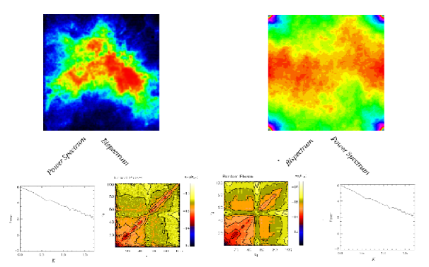
The bispectrum is a complex function which measures both phase and magnitude information between different wave modes. As this is the first application of the bispectrum on the HI data we show in Figure 11 a visual example of the difference between the power spectrum and the bispectrum. This figure shows the original HI column density image of the SMC (top left), and the same image but with manipulated phases (top right). To obtain the top right image we Fourier transformed the SMC image and randomized the phases with a Gaussian random distribution but left the amplitudes the same. Even though the phases of the top images are very different, the power spectrum uses only amplitude information and is identical for both images, as shown in the bottom panels of Figure  11. However, the bispectrum looks very different for the two images, as expected, and offers an insight into the phase information.

In practice, our calculation of the bispectrum involves performing a Fast Fourier Transform (FFT) of the column density functions and the application of Equation 12. We randomly choose wavevectors and their directions, $k_{1}$ and $k_{2}$ and iterate over them, calculating $k_{3}=k_{1}+k_{2}$. We limit the maximum length of the wave vectors to half of the box size. We normalize direction vectors to unity, calculate positions in Fourier space, and finally, compute the bispectrum, which yields a complex 2D array. When plotting the bispectrum (Figures 12-15) we plot bispectral amplitudes, which give information about the degree of mode correlations in the original column density distribution.

Figure 11.— This figure illustrates differences between the bispectrum and the spatial power spectrum. The image at the top left is the original SMC HI column density image, while the image on the right has the same amplitudes however the phases have been randomized with a random Gaussian distribution. As expected, the power spectrum of the two images is identical, but the bispectrum shows a significant difference.

8.2. Bispectrum of MHD Simulations

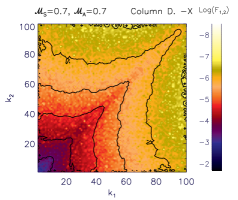
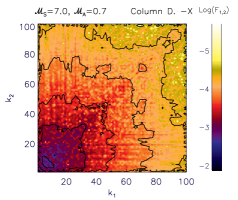
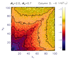
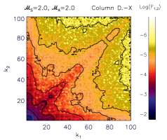
In order to interpret the bispectrum of the SMC HI column density we first compute the bispectrum of the MHD simulations (scaled by the standard score method and without applying cloud boundaries) and look for dependence of wave-wave correlations on the sonic and Alfvén Mach numbers. Figure 12 shows the bispectrum of simulated column density distributions for the case of fixed ${\cal M}_{A}=0.7$ and two extreme cases of ${\cal M}_{s}$: 0.7 and 7.0. In Figure 13 we fix ${\cal M}_{s}=2.0$ and look at two cases of ${\cal M}_{A}$: 0.7 and 2.0.

The first thing to notice in the bispectral contour maps is that the $k_{1}=k_{2}$ case always shows high correlation since this is a trivial case of two wave numbers being the same. For $k_{1}\neq k_{2}$ the bispectral amplitude and isocontour shape vary with turbulent properties but generally amplitude decreases gradually radially from $k_{1}=k_{2}=0$. Models with circularly/broad-shaped isocontours have high amplitudes and wave-wave correlations, while models with more narrow isocontours have lower amplitudes and therefore weaker correlations. For a fixed ${\cal M}_{A}$, supersonic models show a higher degree of wave-wave correlations over subsonic models. For a fixed ${\cal M}_{s}$, models with a higher magnetic field (sub-Alfvénic, e.g. ${\cal M}_{A}=$0.7) show somewhat stronger correlations then the models with a weaker magnetic field (super-Alfvénic) although this difference is not striking.

Figure 12.— The amplitude of the bispectrum for the scaled simulated column density, derived by integrating along the x direction. The left plot shows a subsonic model, while the right plot is for a supersonic model. Both models have ${\cal M}_{A}$=0.7. These figures show the degree of correlation between wavenumbers $k_{1}$ and $k_{2}$. The supersonic model has higher bispectral amplitudes, and more circular isocontours, therefore a stronger correlation between wave modes.

Figure 13.— The amplitude of the bispectrum for the scaled simulated column density. The left plot shows a sub-Alfvénic model, while the right plot is for a super-Alfvénic model. Both models have ${\cal M}_{s}$=2.0. These figures show the degree of correlation between wavenumbers $k_{1}$ and $k_{2}$. While the difference in amplitudes is less pronounced than in the previous figure, the model with a higher magnetic field (i.e. sub-Alfvénic) has more circular isocontours and therefore a slightly enhanced correlations between wave modes.

8.3. Bispectrum of the SMC

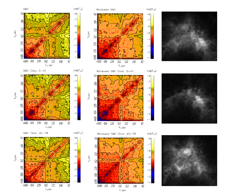
The bispectrum of the SMC HI column density is shown in Figure 14. The top row (first column) shows the bispectrum of the column density derived by integrating all 78 velocity channels. The middle and bottom rows show the bispectrum of the first (for channels 1 to 42) and the last half (for channels 43 to 78) of the data cube. To facilitate interpretation the wavenumbers $k_{1}$ and $k_{2}$ are shown in terms of linear size. While there are small differences in the bispectral amplitudes, there is essentially no significant difference in the contour shape for the three bispectra.

To properly compare the SMC bispectrum with simulations we apply a windowing function on the SMC column density image to simulate the effect of periodic boundaries. We use the Hanning window $w(n)$ function, defined as:

$$w(n)=0.5\left(1-\cos\frac{2\pi n}{N-1}\right)$$ (13)

where $N$ is the number of pixels along the x or y axis, and $n$ ranges from 0 to $N-1$. This windowing function makes the map periodic in the Fourier space. The second column of Figure 14 shows the resultant bispectra for all three cases of HI column density integrations. The windowing seems to slightly change bispectral amplitudes on the large scales, but leaves the general structure of the bispectral contours intact, although some smoothing effects are observed. The increase in large scale correlations is at a level of $\sim 10$%.

Figure 14.— The amplitude of the bispectrum for the SMC HI column density. The left column shows the bispectrum for the scaled unwindowed SMC image, while the right column shows the effects of a Hanning window on the bispectrum. The first row shows the SMC column density image derived by integrating over all 78 velocity channels. The second row is for the image derived by integrating over channels 1-42, while the third row shows the bispectrum of the image obtained by integrating the HI data cube over channels 43-78. The appropriate column density images used to derive the bispectrum are shown in the right-hand column. The bispectrum shows the degree of correlation between wavenumbers $k_{1}$ and $k_{2}$ in at varying depths of integration. We display the bispectral amplitude for spatial scales 4400–80 pc as the bispectrum is very noisy at smaller scales.

Before interpreting the SMC bispectrum we briefly investigate how the presence of noise in the observational data affects the bispectrum. We made the noise image of the HI column density by taking a single velocity channel from the SMC HI data cube without HI emission and integrating this image over the whole velocity range. The bispectrum of the noise image (normalized using the standard score method) is shown in Figure  15 (right). In the case of purely Gaussian noise, we expect a random distribution over the whole space of wavelengths. As a result, the bispectrum will have a gradual increase in amplitude, with the highest amplitude being at large $k$ (or small scale). Figure  15 (left) illustrates this effect for a pure Gaussian distribution. The bispectrum of the SMC noise image shows essentially the same trend, suggesting that we are dealing mainly with Gaussian (random) noise. As is obvious from Figures 12-14, the bispectral amplitude increases in the opposite direction (from large to small scales). The effect of noise is therefore the most important at the smallest spatial scales, and we keep this in mind when interpreting the bispectrum.

Figure 15.— (Left) The amplitude of the bispectrum of a pure Gaussian distribution. It gradually increases from almost zero at small $k$ to $10^{-3}$ at large $k$. (Right) The amplitude of the bispectrum derived for a single emission-less channel from the SMC HI data cube.

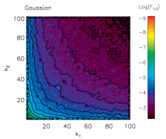
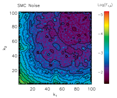
Figure 14 shows the degree of wave-wave correlations in the HI distribution. Modes are obviously strongly correlated at the largest scales and show weaker correlation at small scale. This trend is similar to what was found for various MHD simulations, and obviously very different from the case of Gaussian noise. In addition, the $k_{1}=k_{2}$ line shows the strongest correlations, as is also seen in the simulations. However, contrary to simulations where the level of correlation gradually decreases along this line, we see significant small-scale variations. Several local peaks are noticeable and a strong break at mid-scales. The break occurs around $k_{1}=k_{2}\approx 160$ pc and is seen in all three integrations of the HI data cube. This could be due to a lack of interactions between turbulent eddies at the scale of $\sim 160$ pc, caused possibly by numerous expanding shells in the SMC. Hatzidimitriou et al. (2005) and Stanimirovic (2007) showed that shells in the SMC range in size from 30 to 800 kpc, however the radius distribution peaks at $\sim 60$ pc. The break in the bispectrum may be signifying the lack of correlations on scales close to the typical shell diameter, or some additional physical processes.

We can also compare the bispectrum of the SMC with the bispectra of various simulations. By visual inspection of Figures 12-13, the closest simulation to the SMC in terms of contour shapes is the one for ${\cal M}_{s}=2.0$ and ${\cal M}_{A}=2.0$. Further work in this area is required to derive a real measure to quantitatively compare observed and simulated bispectra.

9. Discussion and Summary

9.1. Turbulence properties of the HI gas in the SMC

Using 3rd and 4th statistical moments of the HI column density image and boothstreping turbulent information from a database of isothermal MHD simulations, we have mapped spatial variations of the sonic Mach number across the SMC. While most of the HI seen in emission in the SMC appears to be subsonic or transonic, several supersonic regions have emerged from our study. It is interesting that these regions do not correlate well with the most recent sites of star formation and seem to point out to large scale shearing or tidal flows. Commonly, it is believed that supernovae and superbubbles are the main drivers of galactic turbulence (McCray & Snow 1979), with a typical size of $\sim 100$ pc. While we do not have high enough resolution to see changes on such small scales ($\sim 10^{\prime}$) in our derived map of ${\cal M}_{s}$, most of the star-forming bar of the SMC appears to have subsonic or transonic properties when viewed at resolution of 30^′.

The most turbulent regions in the SMC may be tracing some kind of shearing flows between the SMC bar and the surrounding HI. This suggests that SMC’s chaotic history with the LMC and our own Milky Way has probably left strong turbulent imprints on the HI gas. The lack of a turnover in the HI spatial power spectrum on the largest observed scales is also indicative of the fact that turbulent energy injection happens largely on scales larger than the size of the SMC Stanimirovic & Lazarian (2001). Similarly, Goldman (2000) suggested that the HI turbulence in the SMC was induced by large-scale flows from tidal interactions with the Milky Way and the LMC about $2\times 10^{8}$ yrs ago. Such large-scale bulk flows could have generated turbulence through shear instabilities, and this turbulence has not have had enough time to decay.

Most of the HI in the SMC has a sonic Mach number of 1-2. This is on average at least two times smaller than what we inferred from HI absorption observations for the CNM in the SMC, ${\cal M}_{s}\sim$3.5-4. Similarly, for the CNM in the Milky Way Heiles & Troland (2003) found ${\cal M}_{s}\sim 3$ with a large dispersion. A sonic Mach number of about 4-5 is commonly assumed for cold gas in molecular clouds (Federrath et al. 2009). For example, Heyer et al. (2006) measured from CO observations ${\cal M}_{s}=4.2\pm 0.17$ for the Rosette molecular cloud, and ${\cal M}_{s}=4.7\pm 0.12$ for G216-2.5. On the other hand, Hill et al. (2008) found that the distribution of the warm ionized medium (WIM) in the Milky Way can be best fit by models for mildly supersonic turbulence with ${\cal M}_{s}\sim 1.4-2.4$. Turbulent properties of the HI in emission in the SMC are therefore closer to properties of the WIM in the Milky Way than properties of the CNM. This may suggest a large fraction of warm relative to cold HI being traced in HI emission.

In the Milky Way, the HI is known to consist of at least two components with different temperature: the WNM with $T_{warm}=6000$ K and the CNM with $T_{cold}=70$ K. In addition, there could be a substantial amount of gas at intermediate temperatures Heiles & Troland (2003). Due to its lower metallicity, the HI in the SMC has different properties. Dickey et al. (2000) found $T_{cold}=40$ K, in agreement with theoretical expectations by Wolfire et al. (1995) whereby the existence of the two-phase medium is possible only at higher pressures compared with the range that applies for solar neighborhood conditions. They also estimated the fraction of cold HI in the SMC to be $\mathrel{\hbox{\hbox to0.0pt{\hbox{\lower 4.0pt\hbox{$\sim$}}\hss}\hbox{$<$}}}15$%. This is lower than $\sim 25$% found for the Milky Way.

As our simulations are isothermal it is obvious to wonder how does the multi-phase HI affect our statistics and conclusions. We investigate this in Figure 16 by producing a simulated data cube from a weighted combination of two cubes, one subsonic (${\cal M}_{s}$=0.7) and one supersonic. The subsonic cube represents contribution from warmer gas, while the supersonic cube represents the cold gas. We combined the two cubes with different emphasis on warm vs cold gas, obtained the column density image of the resultant cube, and calculated its moments.

Figure 16 shows that for the case when the supersonic cube has ${\cal M}_{s}$=2.0 skewness of the final cube with up to 50% of subsonic gas will be biased towards supersonic gas and will appear dominated by cold gas. If we increase the sonic Mach number of the supersonic cube to 4.0, the dominance of the higher turbulence is even more pronounced. A cube with up to 60-70% of subsonic gas and 25% of supersonic gas, will still have high skewness biased by the supersonic contribution. Considering that the HI column density image results in the mean ${\cal M}_{s}=1-2$, significantly lower than what is expected for the cold HI, the fraction of the CNM along any LOS is most likely $\mathrel{\hbox{\hbox to0.0pt{\hbox{\lower 4.0pt\hbox{$\sim$}}\hss}\hbox{$<$}}}25$%. This supports the Dickey et al. (2000) estimate of the fraction of cold HI in the SMC being about 15%.

Figure 16.— Skewness vs. percent of gas that is subsonic for column density of a $512^{3}$cube weighted with supersonic and subsonic gas. Supersonic gas generally dominates the skewness of the column density PDF.

9.2. Is the HI in the SMC sub-Alfvénic or Super-Alfvénic?

Two different statistical approaches in our study suggest that the HI gas in the SMC seen in emission is super-Alfvénic. As we have shown in Figure  10, in addition to the sonic Mach number the spectral slope of the spatial power spectrum is sensitive to the Alfv́enic Mach number for ${\cal M}_{s}<2$. The sub-Alfvénic models generally show steeper slopes due to large scale influence of magnetic fields. Thus, if one independently knows the sonic Mach number, it is possible to estimate the Alfv́enic one using just the column density data. While the dependence of the spectral slope on the Alfv́enic Mach number has not received much attention in the past, it is somewhat expected. Essentially, magnetization decreases compression in the shocks. Strong magnetic forces mix up density clumps preventing formation of isolated peaks, which results in a steeper spectrum. In addition, in the sub-Alfvénic case we expect oblique shocks to be disrupted by Alfvén shearing, which in turn, produces more small scale shocks Beresnyak, Lazarian & Cho (2005).

Another indication that the HI in the SMC is super-Alfvénic comes from the bispectrum. The very sharp decrease in the bispectral amplitudes from large to small scales observed for the SMC is the closest to the trend found for simulated data for the case of ${\cal M}_{s}\sim 2$ and ${\cal M}_{A}\sim 2$. Detailed comparison between simulated and observed bispectra awaits future work, however this qualitative comparison is certainly encouraging.

Assuming on average ${\cal M}_{s}\sim 1-2$, the power spectrum slope suggests a super-Alfvénic HI in the SMC with ${\cal M}_{A}\sim 1-3$. This is generally in agreement with the observationally inferred strength of the magnetic field by Mao et al. (2008). Using their estimate for $B_{\rm ext}=2$ $\mu$G, a radius of the SMC of 2 kpc, the total hydrogen mass of $4.2\times 10^{9}$ M_⊙, and a typical velocity dispersion of 20 km s^-1(Stanimirovic et al. 2004), we estimate ${\cal M}_{A}\sim 3$. As the Alfv́enic Mach number shows the nature of the interplay between gas pressure and magnetic fields, it appears that the gas pressure in the SMC dominates over the magnetic pressure.

9.3. Intermittency in mode correlations?

Our bispectrum analysis of the SMC HI data was the first attempt to apply bispectrum on observed astrophysical data. While more detailed comparison between observations and simulations awaits future work, we clearly see trends in the bispectral amplitudes similar to what was found for simulations of supersonic MHD turbulence. The most interesting finding is, however, the effect of small-scale variations in the $k_{1}=k_{2}$ correlations and a strong break in correlations at a scale of 160 pc. Such small-scale variations, or jumps, have not been seen in the bispectrum of simulated data. We can speculate about several possible scenarios that could explain their existence. The jumps could be caused by the energy injection due to processes other than turbulence affecting specific spatial scales. Alternatively, the jumps may be marking the presence of colder or multi-phase gas. Similarly, the observed break in the bispectrum at about 160 pc is intriguing. As we already pointed out, it is interesting that most expanding shells in the SMC (more than 500 were cataloged so far) have a diameter of $\sim 120$ pc. The break could be due to the lack of correlations on scales similar to the distance between two shell centers. Obviously this will require further studies.

9.4. Limitations of the present study

A natural question to ask is how results presented in this paper depend on the resolution of numerical simulations. For example, Kritsuk et al. (2007) investigated how resolution of numerical simulations affects the power spectrum of density. These authors found that the spectral index estimates based on low resolution simulations bear large uncertainties due to the bottle neck contamination, and that the power spectra of $512^{3}$ simulations are substantially shallower then models with resolution of $1024^{3}$. However, while Kritsuk et al. (2007) only examined hydrodynamic turbulence, Beresnyak et al. (2008) showed that the slopes were very different between the MHD and pure hydrodynamic cases. For instance, the slopes for hydrodynamic simulations showed a pronounced and well defined bottleneck effect, while the MHD slopes were much less affected. This is indicative of MHD turbulence being less local than the Kolmogorov turbulence, and suggests that our simulations will be less affected by resolution. In addition, Kritsuk et al. (2007) found a difference in the slope between hydrodynamic $512^{3}$ and $1024^{3}$ simulations to be 0.17. This would result in a change of $d{\cal M}_{s}\sim 0.5$ only and will not change our interpretation. We also add that in the case of higher statistical moments and the bispectrum BFKL confirmed trends noticed by KLB at lower resolution of 128³.

Another issue that should be further addressed and that could affect our results is the type of numerical forcing of turbulence. Federrath et al. (2009) recently investigated the effects of solenoidal vs. compressive (divergence-free vs. curl-free) forcing on a variety of statistics including PDFs and higher order moments. They found that both types of driving mechanisms are compatible with observations of molecular clouds however, depending on the data studied, one type could be superior then the other in terms of the statistics and reproduced observables. This implies that different regions in the SMC may exhibit statistical signatures of either compressive or solenoidally driven turbulence.

9.5. Summary

We have investigated a new method for constraining turbulent properties of the ISM, specifically the sonic Mach number, by using the HI column density image and a database of numerical simulations with a range of sonic and Alfv́enic Mach numbers. By applying the 3rd and 4th statistical moments on both observed and simulated data we have derived the spatial distribution of the sonic Mach number across the SMC with angular resolution of 30^′. To provide an estimate of the Alfv́enic Mach number we used two approaches: the spatial power spectrum and the bispectrum. Using the database of numerical simulations we have shown that the spatial power spectrum varies with both the sonic and Alfv́enic Mach numbers. If the sonic number is known the Alfv́enic number can be constrained from this dependence. The bispectrum shows the level of correlation between turbulent eddies of different size and depends greatly on the sonic Mach number, and somewhat on the Alfv́enic Mach number. By comparing the bispectra of observations and simulations we have gauged the importance of magnetic fields relative to the gas pressure in the SMC. The following results were discussed in the paper.

• Skewness and kurtosis of the HI column density generally correlate well and are within the range expected from MHD simulations. This suggests that departures from Gaussianity could be interpreted as being governed by MHD turbulence.

• Most of the HI in the SMC bar and the Eastern Wing is subsonic or transonic with ${\cal M}_{s}\sim 0-2$. Sites of most recent star formation have ${\cal M}_{s}\sim 1$. Regions with the highest skewness and kurtosis, which could be interpreted as having ${\cal M}_{s}\sim 4$, correspond to the edges of the bar. The most turbulent regions are most likely tracing tidal or shearing flows. The fraction of the SMC with different turbulent properties is: 10% with ${\cal M}_{s}>2$, 80% with $0<{\cal M}_{s}<2$, and about 10% with very low values of ${\cal M}_{s}$.

• Using HI absorption profiles from Dickey et al. (2000) we have estimated that the CNM in the SMC is highly supersonic with ${\cal M}_{s}=3.5-4$. This is at least a factor of two higher than what we measured from the higher statistical moments for the HI gas seen in emission. One possible reason for this discrepancy could be that HI emission is dominated by warm gas and the fraction of the CNM in the SMC is $\mathrel{\hbox{\hbox to0.0pt{\hbox{\lower 4.0pt\hbox{$\sim$}}\hss}\hbox{$<$}}}20$%.

• The slope of the spatial power spectrum and the bispectrum suggest that the HI in the SMC is super-Alfv́enic with ${\cal M}_{A}\sim 1-3$. This is implies that the gas pressure dominates over the magnetic pressure.

• The bispectrum of the HI column density shows large scale wave correlations suggesting a large scale energy injection mechanism. Contrary to simulations which show a smooth decrease of wave-wave correlations from large to small scales, the SMC bispectrum shows localized enhancements of correlations and at least one prominent break at $\sim 160$ pc. We speculate that the multi-phase medium, and/or energy injection by processes other than turbulence, could be responsible for the correlation jumps. The break on the other hand appears at a scale similar to the diameter of the majority of expanding shells in the SMC.

Figure 17.— Kurtosis vs. Skewness for isothermal simulations. The left is subsonic while the right is supersonic. These figure are similar to 5 except that the beam was modified with 7 extra points set to zero. The supersonic models remain relatively unchanged in their trend while subsonic models with the modified distribution obtain a very tight anti-correlation due to extra points pushing them away from Gaussianity. The supersonic model is unaffected because it is already very positively skewed. This could be employed as an additional method to detect subsonic gas using moments

Figure 18.— Kurtosis and Skewness map with beams modified with 7 zero points side by side. Areas where they do not agree in sign (dark blue in skewness and dark blue/red in kurtosis) point to anti-correlation , which indicates regions that are potentially subsonic. These regions correspond to areas of low kurtosis and skewness in the previous maps, yet are more clearly seen here. The largest of these subsonic regions is seen along the bridge between the bar and the east wing (See Figure 5).

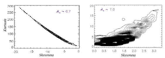
In Figure 17 we plot kurtosis vs. skewness in a manner similar to Figure 5. The difference between this figure and Figure 5 is that we added seven zero points into the beam (instead of 3841 points there are now 3848 points). This produces almost no change in the supersonic models since they already have high positive skewness and kurtosis. Supersonic models still show strong correlation between skewness and kurtosis.

However a big change is seen in the subsonic skewness vs. kurtosis. The additional zero points shift the distribution from Gaussian (the mean of our simulations with no scaling applied is unity) to negative skewness and very peaked kurtosis producing a tight anti-correlation. Because this technique only strongly affects subsonic areas we can use it to locate subsonic turbulence in the SMC with skewness and kurtosis by looking for anti-correlation and very high values. These properties also hold for simulations with cloud boundaries imposed. Note that one must use caution here and carefully examine the distribution of data.

The application of this technique to the SMC data is shown in Figure 18. This plot shows the skewness and kurtosis maps of the SMC side by side with the modified beam. Indeed, most regions are unchanged from the analysis in Section 5. However a few regions stick out with signatures that are subsonic, that is, anti-correlation between skewness and kurtosis. Two regions of the highest kurtosis are located in the area between the HI bar and the Eastern Wing. While kurtosis reaches values of 4-8, the corresponding skewness values are negative, $\sim-1$. Again, such combination of skewness and kurtosis may correspond to simulations of subsonic isothermal MHD turbulence, and/or points out additional processes at work.

References

- Beresnyak, Lazarian & Cho (2005) Beresnyak, A., Lazarian, A. & Cho, J., 2005, ApJ, 624, L93
- Biskamp (2003) Biskamp, D. (2003), Magnetohydrodynamical Turbulence, (Cambridge University Press, Cambridge).
- Brunt & Heyer (2002) Brunt, C., & Heyer, M.,2002,ApJ, 566, 27
- Burkert (2006) Burkert, A., 2006, C. R. Physique 7
- Burkhart et al. (2009) Burkhart, B. Falceta-Goncalves, D., Kowal, G., Lazarian, A., 2009, ApJ, 693, 250 (BFKL)
- Cho & Lazarian (2002) Cho, J. & Lazarian, A. 2002, Phys. Rev. Lett., 88, 5001
- Cho & Lazarian (2003) Cho, J. & Lazarian, A., 2003, MNRAS, 345, 325
- Chepurnov & Lazarian (2009) Chepurnov, A., & Lazarian, A., 2009, ApJ, 693, 1074
- Chepurnov et al. (2008) Chepurnov, A., Lazarian, A., Gordon, J., & Stanimirovic., S., ApJ, 688, 1021
- Crovisier & Dickey (1983) Croviser, J., & Dickey, M., 1983, A&A, 122, 282
- Deshpande (2000) Deshpande et al.,2000, ApJ, 543, 227
- Dickey et al. (2000) Dickey et al., 2000, ApJ, 536, 756
- Elmegreen & Scalo (2004) Elmegreen, B., & Scalo, J., ARA&A, 42, 211
- Esquivel & Lazarian (2005) Esquivel, A., & Lazarian, A., 2005, ApJ, 631, 320
- Esquivel & Lazarian (2009) Esquivel, A., & Lazarian, A., 2009, ApJ in press
- Esquivel et al. (2003) Esquivel, A., Lazarian, A., Pogosyan, D., & Cho, J., 2003, MNRAS, 342, 325
- Esquivel et al. (2007) Esquivel et al., 2007, MNRAS, 381, 1733
- Federrath et al. (2009) Federrath, C., et al.,2009, AA, in press
- Fry (1998) Fry, J. N. 1998, Annals of the New York Academy of Sciences 848, 62
- Gill & Henriksen (1990) Gill, A.G., & Henriksen, R.N., 1990, ApJ, 365, L27
- Goodman et al. (2009) Goodman, A. et al.,2009, ApJ, 692, 91
- Hatzidimitriou (2005) Hatzidimitriou et al., 2005, MNRAS, 360,1771
- Heiles & Troland (2003) Heiles, C., Troland, T., 2003, ApJ, 586, 1067
- Heyer & Zwiebel (2004) Heyer, M., & Zwiebel, E., 2004, Ap&SS, 292, 9
- Hill et al. (2008) Hill, A. S., Benjamin, R. A., Kowal, G., Reynolds, R. J., Haffner,. L. M. & Lazarian, A., 2008, ApJS
- Intrator et al. (1989) Intrator, T., Meassick, S., Browning, J., Majeski, R. & Hershkowitz, N. 1989, Phys. Fluids B, 1, 271-273
- Kennicutt (1995) Kennicutt et al. 1995, AJ, 109, 594
- Kowal, Lazarian & Beresnyak (2007) Kowal, G., Lazarian, A. & Beresnyak, A., 2007, ApJ, 658, 423 (KLB)
- Kowal et al. (2009) Kowal et al., 2009, ApJ, 700,63
- Kritsuk (2007) Kritsuk et al., 2007, ApJ, 665, 416
- Lazarian (2007) Lazarian, A., 2007, JQSRT, 106, 225
- Lazarian (2009) Lazarian, A., 2009, SSR, 143, 357
- Lazarian et al. (2001) Lazarian et al.,2001, ApJ, 555, 130
- Lazarian & Pogosyan (2004) Lazarian, A. & Pogosyan, D., 2004, ApJ, 616, 943
- Lazarian & Pogosyan (2006) Lazarian,A. & Pogosyan,D., 2006,ApJ, 652, 1348
- Lazarian & Pogosyan (2000) Lazarian, A. & Pogosyan,D., 2000, ApJ, 537, 720
- Lazarian & Vishniac (1999) Lazarian, A., & Vishniac, E., 1999, ApJ, 511, 193
- Levy, Puppo & Russo (1999) Levy, D., Puppo, G. & Russo, G., 1999, Mathematical Modeling and Numerical Analysis, 33, 547
- Liguori et al. (2006) Liguori, M., Hansen, F. K., Komatsu, E., Matarrese, S. & Riotto, A., 2006, PhRvD, 73, 3505
- Lithwick & Goldreich (2001) Lithwick, Y. & Goldreich, P., 2001, ApJ, 562, 279
- Liu & Osher (1998) Liu, X.-D. & Osher, S., 1998, Journal of Computational Physics, 141, 1
- Mao et al. (2008) Mao et al. 2009, ApJ, 688, 1029
- McCray & Snow (1979) McCray, R.,& Snow, P, 1979, A&AA, 17, 213
- McKee & Ostriker (2007) McKee, C., Ostriker, E., 2007,
- Monin, A.S.& Yaglom, A.M. (1967) Monin, A.S.& Yaglom, A.M.,1967, Statistical Fluid Mechanics, MIT Press
- Montgomery et al. (1987) Montgomery, D., Brown, M. R., Matthaeus, W. H., 1987, J. Geophys. Res., 92, 282
- Nordlund & Padoan (1999) Nordlund, A. K. & Padoan, P., 1999, Interstellar Turbulence, proceedings of the 2nd Guillermo Haro Conference, Cambridge University Press
- Ostriker et al. (2001) Ostriker, E. C., Stone, J. M. & Gammie, C. F., 2001, ApJ, 546, 980
- Scoccimarro (2000) Scoccimarro, R., 2000, ApJ, 544, 597
- Stanimirovic et al. (1999) Stanimirovic, S., Staveley-Smith, L., Dickey, J. M., Sault, R. J., & Snowden,S. L., 1999, MNRAS, 302, 417 (SX99)
- Stanimirovic & Lazarian (2001) Stanimirovic, S. & Lazarian, A., 2001, ApJ, 551, L53
- Stanimirovic (2001) Stanimirovic, S., 2001, Astrophysics and Space Science, 277, 87
- Stavely-Smith et al. (1997) Staveley-Smith, L., Sault, R. J., Hatzidimitriou, D., Kesteven, M. J., & McConnell, D. 1997, MNRAS, 289, 225
- Stanimirović& Staveley-Smith (2004) Stanimirović, S., Staveley-Smith, L., & Jones, P. A. 2004, ApJ, 604, 176
- Stanimirović (2007) Stanimirović, S.,2007, IAU Symposium, 237, 84 Stutzki, J., Bensch, F., Heithausen, A., Ossenkopf, V., & Zielinsky, M., 1998, A&A, 336, 697
- Tabachnick & Fidell (1996) Tabachnick, B. G., & Fidell, L. S. (1996). Using multivariate statistics (3rd ed.). New York: Harper Collins.
- Tynan et al. (2001) Tynan, G. R., Moyer, R. A., Burlin, J. & Holland, C. 2001, Phys. Plasmas, 8, 2691
- Westerlund (1991) Westerlund, B. E. 1991, in The Magellanic Clouds, IAU Symp., 148, 15