A posteriori inclusion of parton density functions in NLO QCD final-state calculations at hadron colliders:
The APPLGRID Project
Abstract
A method to facilitate the consistent inclusion of cross-section measurements based on complex final-states from HERA, TEVATRON and the LHC in proton parton density function (PDF) fits has been developed. This can be used to increase the sensitivity of LHC data to deviations from Standard Model predictions. The method stores perturbative coefficients of NLO QCD calculations of final-state observables measured in hadron colliders in look-up tables. This allows the a posteriori inclusion of parton density functions (PDFs), and of the strong coupling, as well as the a posteriori variation of the renormalisation and factorisation scales in cross-section calculations. The main novelties in comparison to original work on the subject are the use of higher-order interpolation, which substantially improves the trade-off between accuracy and memory use, and a CPU and computer memory optimised way to construct and store the look-up table using modern software tools. It is demonstrated that a sufficient accuracy on the cross-section calculation can be achieved with reasonably small look-up table size by using the examples of jet production and electro-weak boson (, ) production in proton-proton collisions at a center-of-mass energy of TeV at the LHC. The use of this technique in PDF fitting is demonstrated in a PDF-fit to HERA data and simulated LHC jet cross-sections as well as in a study of the jet cross-section uncertainties at various centre-of-mass energies.
1 Introduction
The Large Hadron Collider (LHC) at CERN will collide protons at a centre-of-mass energy of up to GeV. The combination of its high collision rate and centre-of-mass energy will make it possible to probe new interactions at very short distances. Such interactions might be revealed in the production of cross-sections of particles at very high transverse momentum () as a deviation from the Standard Model theory.
The sensitivity to new physics depends on experimental uncertainties in the measurements and on theoretical uncertainties in the Standard Model predictions. It is therefore important to work out a strategy to minimise both the experimental and theoretical uncertainties from LHC data. Residual renormalisation and factorisation scale uncertainties in next-to-leading order (NLO) QCD calculations for single inclusive jet cross-sections are typically about and should hopefully be reduced as NNLO calculations become available. However, in some kinematic regimes, PDF uncertainties can be substantially larger than the uncertainties from higher-order corrections, for example at large . One strategy to reduce such uncertainty is to use single inclusive jet or Drell-Yan cross-sections at lower to constrain the proton parton density function (PDF) uncertainties at high .
In order to further constrain PDF uncertainties, it would be useful to be able to include final state data such as and rapidity distributions for -boson and jet production in global NLO QCD PDF fits, without recourse to inexact methods like the use of simple factor correcting of LO cross-sections (factors). We propose here a method for a consistent inclusion of final-state observables in global QCD analyses.
For inclusive data, like the proton structure function in deep-inelastic scattering (DIS) the perturbative coefficients are known analytically. During the fit the cross-section can therefore be quickly calculated from the strong coupling () and the PDFs and then be compared to the measurements. However, final state observables, where detector acceptances or jet algorithms are involved in the definition of the perturbative coefficients (called “weights” in the following), have to be calculated using NLO QCD Monte Carlo programs. Typically such programs need about one day of CPU time to accurately calculate the cross-section. It is therefore necessary to find less time consuming methods.
Any NLO QCD calculation of a final-state observable involves Monte Carlo integration over a large number of events. For deep-inelastic scattering and at hadron colliders this must usually be repeated for each new PDF set, making it impractical to consider many ‘error’ PDF sets, or carry out PDF fits. Here, the “a posteriori” inclusion of PDFs is discussed, whereby the Monte Carlo run calculates a look-up table (in momentum fraction, , and momentum transfer, ) of cross-section weights that can subsequently be combined with an arbitrary PDF. The procedure is numerically equivalent to using an interpolated form of the PDF.
Many methods have been proposed to solve this problem in the past [1, 2, 3, 4, 5]. In principle the highest efficiencies can be obtained by taking moments with respect to Bjorken- [1, 2], because this converts convolutions into multiplications. This can have notable advantages with respect to memory consumption, especially in cases with two incoming hadrons. On the other hand, there are complications such as the need for PDFs in moment space and the associated inverse Mellin transforms.
Methods in -space have traditionally been somewhat less efficient, both in terms of speed and in terms of memory consumption. They are, however, somewhat more transparent since they provide direct information on the values of relevance. Furthermore they can be used with any PDF. The use of -space methods can be further improved by using methods developed originally for PDF evolution [6, 7, 8].
Our method [9] bears a number of similarities to that of the fastNLO project [10] and the two approaches were to some extent developed in parallel. Relative to fastNLO, we take better advantage of the sparse nature of the -dependent weights, allow for more flexibility in the scale choice by keeping explicitly the scale dependence as an additional dimension in the weighting table and provide a means to evaluate renormalisation and factorisation scale-dependence a posteriori. We also provide a broader range of processes, since in addition to di-jet production, we include W- and Z-boson production. In order to make easy use of the large number of weight files for practically all inclusive jet spectra and di-jet mass spectra made available by the fastNLO project, we provide a software interface to make use of these weight tables within the APPLGRID framework.
2 PDF-independent representation of cross-sections
2.1 Representing the PDF on a grid
We make the assumption that PDFs can be accurately represented by storing their values on a two-dimensional grid of points and using -order interpolations between those points. Instead of using the parton momentum fraction and the factorisation scale , we use a variable transformation that provides good coverage of the full and range with uniformly spaced grid points:
| (1) |
The parameter should be chosen of the order of , but need not necessarily be identical. The parameter serves to increase the density of points in the large region111For a fixed total number of bins, as the bins at large get finer, the low- ones become wider. and can be chosen according to the needs of the concrete application.222In case of the function is analytically invertible, for a numerical inversion has to be applied.
The PDF is then represented by its values at the 2-dimensional grid point , where and denote the grid spacings, and is obtained elsewhere by interpolation:
| (2) |
where , are the interpolation orders. The interpolation function is 1 for , and otherwise is given by:
| (3) |
Defining to be the largest integer such that , and are defined as:
| (4) |
Given finite grids whose vertex indices range from, , for the grid and, , for the grid, one should additionally require that eq. (2) only uses available grid points. This can be achieved by remapping, , and, .
2.2 Representing the final state cross-section weights on a grid (DIS case)
To illustrate the method we take the case of a single flavour in deep-inelastic scattering (DIS).
Suppose that we have an NLO Monte Carlo program that produces events, . Each event has an value, , a value, , as well as a weight, . We define as the number of powers in the strong coupling in event . Normally one would obtain the final result of the Monte Carlo integration for one sub-process from:333Here, and in the following, renormalisation and factorisation scales have been set equal for simplicity.
| (5) |
where is the PDF of the flavour under consideration.
Instead one introduces a weight grid and then for each
event one updates
a portion of the grid with:
| (6) | |||
The final result for , for an arbitrary PDF and an arbitray , can then be obtained subsequent to the Monte Carlo run:
| (7) |
where the sums with indices and run over the number of grid points and we have explicitly introduced and such that:
| (8) |
2.3 Including renormalisation and factorisation scale dependence
If one has the weight matrix determined separately order by order in , it is straightforward to vary the renormalisation and factorisation scales a posteriori (we assume that they were set equal in the original calculation).
It is helpful to introduce some notation related to the DGLAP evolution equation:
| (9) |
where the and are the LO and NLO matrices of DGLAP splitting functions that operate on vectors (in flavour space) of the PDFs. Let us now restrict our attention to the NLO case where we have just two values of in eq. 7. For example, in jet production in DIS, and . Introducing and corresponding to the factors by which one varies and respectively, for arbitrary and we may then write:
| (10) | |||
where and () is the number of colours (flavours). Though this formula is given for an -space based approach, a similar formula applies for moment-space approaches. Furthermore it is straightforward to extend it to higher perturbative orders.
To obtain the full DIS cross-section a summation of the weights and the parton densities over the contributing sub-processes is required.
2.4 The case of two incoming hadrons
In hadron-hadron scattering one can use analogous procedures but with one more dimension. Besides , the weight grid depends on the momentum fractions of the first () and second () hadrons.
The analogue of eq. 7 is given by:
| (11) |
where is the number of sub-processes and the initial state parton combinations are specified in eqs. 2.4.1, 20 and 18.
The combinations of the incoming parton densities (defining the number of sub-processes) often can be simplified by making use of the symmetries in the weights. In the case of jet production only seven sub-processes are needed (see section 2.4.1). The case of -boson and -boson production is treated in the Appendix A. The case of -quark production is discussed in ref. [11].
An automated way to find the sub-processes is discussed in Appendix B.
2.4.1 Sub-processes for jet production in hadron-hadron collisions
In the case of jet production in proton-proton collisions the weights generated by the Monte Carlo program can be organised in seven possible initial-state combinations of partons:
| (12) |
where denotes gluons, , quarks and , quarks of different flavour, and we have used the generalised PDFs defined as:
| (13) | |||||
where is the PDF of flavour for hadron and () denotes the first or second hadron.444 In the above equation and in the following we follow the standard PDG Monte Carlo numbering scheme [12], where gluons are denoted as , quarks have values from - and anti-quarks have the corresponding negative values.
2.5 Including scale dependence in the case of two incoming hadrons
It is again possible to choose arbitrary renormalisation and factorisation scales. Specifically for NLO accuracy:
| (14) | |||
where is calculated as , but with replaced with , and analogously for .
2.6 Reweighting to a different center-of-mass energy
From a weight grid calculated at a particular centre-of-mass energy it is also possible to calculate a cross-section at a different centre-of-mass energy by using transformed parton momentum fractions and adding a flux factor in the cross-section convolution as given by eq. 11 or eq. 2.5:
| (15) |
and the momentum fractions in the generalised parton densities are replaced by:
| (16) |
When it can occur that or , in which case the parton densities should be set to zero. One should be aware that a jet transverse momentum that corresponds to moderate values with centre-of-mass energy (and correspondingly low density of grid points in ) may correspond to large when using a smaller . In such cases, it can happen that the low density of grid points in is no longer sufficient, given that PDFs vary more rapidly at large than at moderate .
Special care is also needed when taking insofar as there will be kinematic regions accessible with the larger values that were not probed at all in the original NLO calculation at centre-of-mass energy . As a concrete example, with , there can be events with three jets having respectively . Such events contribute to the inclusive jet spectrum at . However, taking a grid calculated with (where such events are kinematically disallowed) and using it to determine the inclusive jet spectrum with , this kind of contribution will be left out.
3 Technical implementation
To test the scheme discussed above, the NLO QCD Monte Carlo programs NLOJET++ [13] for jet production and MCFM [16, 17] for the production of - and -boson are used. To illustrate the performance of the method jet and - and -boson production are used as examples. However, it is worth noting that these these two programs give access to many of the NLO QCD calculations presently available.
The weight grid of eq. 11 is filled (for each cross-section bin) in the user module of the NLO program, where one has access to the event weights and the partons’ momenta. This object is called “grid” in the following. At this point the cross-section definition is specified and the physical observables that are being studied are defined (e.g. using a jet algorithm).
The weight grid for each value of the observable in question is represented as a multidimensional object with one dimension each for , and , one for the sub-process in question, and one for the order in . The task is to store the weight grid in such a way that as little memory as possible is used and the information can be extracted in a fast way. In the following several options to reduce the necessary memory are discussed:
The simplest structure for a software implementation of the weight grid is a multidimensional array (for , and ), like the TH3D-class available in the ROOT analysis framework.
The overhead of storing empty bins can be largely reduced by calculating the , and boundaries of the weight grid using the NLO QCD program in a special run before the actual filling step. At the beginning of the filling step the adjusted boundaries of the weight grids are then read-in and an optimised weight grid is constructed.
Since the rectilinear region bounded by limits in , and may contain many phase-space points that are unoccupied, additional memory can be saved by using methods to avoid storing elements in the weight grid that are not filled. Since the occupied regions are continuous, but irregular, grid formats for truly sparse matrices (such as the Harwell-Boeing format) are not used. Instead a custom format is favoured where the grid, lower- and upper-limits in each dimension are stored along with all the elements in between.
This is illustrated in Fig. 1 for a simple two-dimensional grid. For the three-dimensional structure, each of the row-column elements would itself be a column with its own lower and upper range delimiters. The resulting saving of memory is usually around a factor of four, even after taking into account the additional storage for the range delimiters.555 If additional savings are required in the future, packing the range delimiters for each sparse one dimensional structure into a single integer will halve this additional overhead, but will slightly increase the access time due to the unpacking.

Since the grid itself knows the index of the first and last filled element in each row, column etc., it is possible to only iterate over those elements of the grid that contain data. Similarly when interrogating the grid for the value of an element, it is possible to ascertain whether the element is in the occupied, or unoccupied region of the grid and return the value of the filled element if filled, or 0 otherwise. This makes accessing the unfilled members of the grid much faster than otherwise.
The actual implementation for the grid666 The complete code including the interfaces to NLOJET++ and MCFM is available from http://svn.hepforge.org/applgrid. involves a number of related classes written in C++777A FORTRAN interface is also available so that the basic functionality can be accessed from within user FORTRAN code.. The grid for a given cross-section is represented by a concrete instance of a master class, appl::grid. This class has a number of constructors that allow the cross-section it will calculate to be defined in terms of a fixed number of regular or variable width bins in the cross-section observable.
For each bin in the observable, the master class has a number of instances of an internal class – one for each order of – so that for a cross-section with bins, with contributions at leading order and next-to-leading order, the master class would contain a total of instances of the internal class.
This internal class, appl:igrid, encodes all the information required to create the cross-section, at one particular order, for that bin. The class contains the -to-, -to- and -to-, -to- transform pairs, and a subclass that encodes information on how to generate the generalised internal sub-processes for the particular interaction from the basic parton distribution functions. It also contains instances of the sparse grid class in , and described above, for each of the sub-process.
When requested to perform the convolution, the master class calls the convolute method of the subclass for each order of the cross-section in each bin. The convolute method of the subclass performs the convolution over , and for each of the sub-processes.
For each bin in the observable, the master class takes the cross-sections from the subclasses for each order from each bin and adds them to arrive at the final cross section for that bin.
The subclass for the generalised internal sub-processes are very basic classes which encode the number of sub-processes, i.e. seven in the case of jet production, and twelve in the case of -boson production, and simply take the 13 parton distribution values for each incoming hadron at a given scale, and generate the internal processes from these.
When the grid is saved to a ROOT file888Technically, the grid is transformed to TH3D-histograms that are stored in the output ROOT file. the master class encodes the complete status of the internal grids, which transform pair, and which sub-process is required etc., so that once reading from the file, everything required to calculate the cross section (e.g. sub-process definition, CKM matrix elements etc.) is available. In this way all information to perform the cross-section calculation is available from the output file from a single function call by the user and the only additional information required is an input function for generating the PDFs and another one for calculating . We use the HOPPET program [8] to calculate the DGLAP splitting functions needed for the cross-section convolution when the renormalisation and factorisation is varied (see eq. 2.3).
All the various choices in the weight grid architecture and other information needed to calculate the cross-section are encoded in the output file. They are described in the following:
-
•
The centre-of-mass energy at which the weight grid has been produced.
-
•
The choice of the coordinate transform function. By default the form of eq. 1 is used. However, any other function can be provided by the user.
-
•
The interpolation order as given by eq. 2.
-
•
The number of grid points to be used for each dimension , and .
-
•
The definition of the sub-processes via a x matrix.
-
•
The CKM matrix elements or other constants needed to calculate the cross-sections.
-
•
The required number of the points on the grid can be optionally reduced with the aid of reweighting factor in the filling step. This flattens out the PDF in the region where it is steeply falling.
By default the following functional form is used for the reweighting999Such a PDF reweighting was first introduced in ref.[10].:
(17) The parameter can be adjusted to flatten out the change of the PDF at low- while the parameter can be optimised for the high- region. The factor prevents the weight from being zero for .
Reasonable values for the parameters and have been determined by fitting the sum of the up, down and gluon PDFs. For the CTEQ6 PDFs [18], values of to and to have been found for the range GeV. The variation comes from a slight dependence of the and parameters on . For other PDFs, the results of the fit can be slightly different.
The user can change the parameters or provide another functional form.
4 Accuracy of the weight grids
The choice of the weight grid architecture depends on the required accuracy, on the exact cross-section definition and on the available computer resources. For each possible application the weight grid architecture has to be carefully chosen in order to achieve the required accuracy with the available computer memory and computing time. For instance, for observables where the PDFs are steeply falling, e.g. the inclusive jet cross-section at high transverse momentum in the forward region, a fine grid in is needed. The memory usage of weight grids for one cross-section should be kept small since, e.g. in global PDF fits, it might be necessary to read in a large number of weight grids. In addition, the convolution time depends on the number of grid nodes, and so keeping memory requirements as small as possible is in any case desirable. The number of points needed in the weight grid is kept modest by using the higher-order interpolation functions of eq. 2, and optionally also by introducing a PDF weight, as in eq. 17 during the filling step, or by using a sparse structure.
In the following, the influence of the grid architecture on the achievable accuracy in the cross-section calculation is discussed. The computer memory use and execution speed are also investigated. The production of jets and of - and -bosons at LHC are used as examples.
In our test runs, to be independent from statistical fluctuations (which can be large, in particular in the NLO case), in addition to the weight grid, reference histograms are filled using the NLO QCD calculation without weights in the standard way. The result obtained from the weight grid is then compared to these reference histogram.

4.1 Jet production at hadron colliders
The single inclusive jet cross-section as a function of the jet transverse momentum () is calculated for jets in the central rapidity () region of and in the forward rapidity region of . Jets are defined via the seedless cone jet algorithm as implemented in NLOJET++, which corresponds to the seedless algorithm of ref. [19] (or SISCone [20]), except for small differences in the split–merge procedure which are irrelevant at this order. The cone radius has been set to , the overlap fraction to .101010 These choices are related to the fact that some of the NLOJET++ runs were performed some time in the past. A modern cone-algorithm (in the class of those with a split–merge procedure) would be SISCone [20], and a value of would be recommended [21]. The renormalisation and factorisation scales are set to , where is the of the highest jet in the required rapidity region111111 Note that beyond LO the will in general differ from the of the other jets, so when binning an inclusive jet cross-section, the of a given jet may not correspond to the renormalisation scale chosen for the event as a whole. For this reason separate grid dimensions for the jet and for the renormalisation scale are used. This requirement has been efficiently circumvented in some moment-space approaches [2]..
To discuss the dependence of the weight grid performance on the grid architecture, a default weight grid is defined from which variations in a single parameter are studied systematically. The default weight grid consists of bins in and bins in . The points are distributed according to eq. 1 with and th order interpolation is used. No PDF reweighting (see eq. 17) is used.
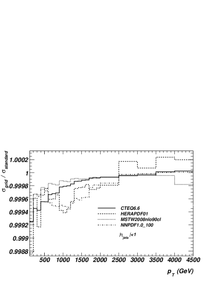
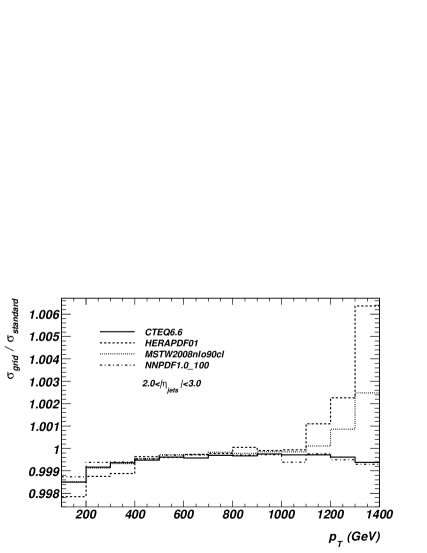
The ratio of the cross-section calculated with the default weight grid to the reference cross-section calculation is shown in Fig. 2 for the jet cross section in the central rapidity region () (a) and the forward rapidity region () (b). The weight grid is produced in a run where the CTEQ6mE PDF [18] has been used to calculate the jet cross-section. This PDF is used as standard in the following. To show the independence of the weight grid performance on the used PDF, Fig. 2 also includes more recent PDFs based on the analyses of a large variety of data (global analysis) like CTEQ6.6 [22] and MSTW2008 [23] or only using inclusive DIS data based on combined H1 and ZEUS data (HERAPDF01) [24]. In addition, we include a PDF that does not use a parameterised input distribution NNPDF [25]. Further comparisons of the jet cross-sections calculated with these PDFs can be found in section 5.
In the central region the cross-section calculated with the weight grid reaches an accuracy of about % for all tranverse jet momenta and all PDFs. In the forward region a similar performance is achieved for transverse jet momenta up to GeV. For transverse jet momenta above that value the performance degrades to and a variation with the PDF is observed.
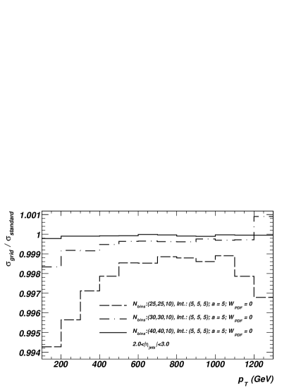
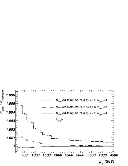
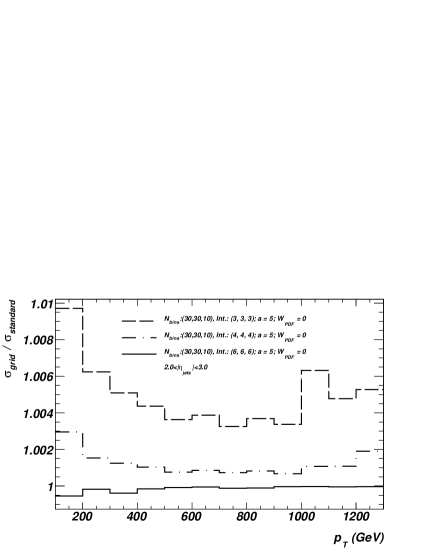
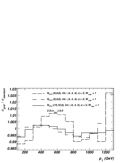
The dependence of the accuracy on the number of -bins is illustrated in Fig. 3. If only -bins are used, the accuracy is in the central and in the forward rapidity region. The accuracy decreases towards low jet transverse momenta. More accuracy is achieved by a larger number of -bins. For bins the accuracy is . For -bins the improvement is small, but visible. A very sensitive kinematic region is the forward region with very high transverse momenta. In this region at least -bins are needed to get an accuracy of .
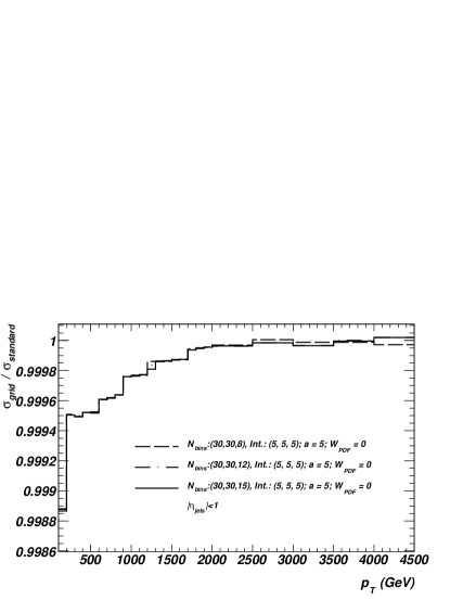
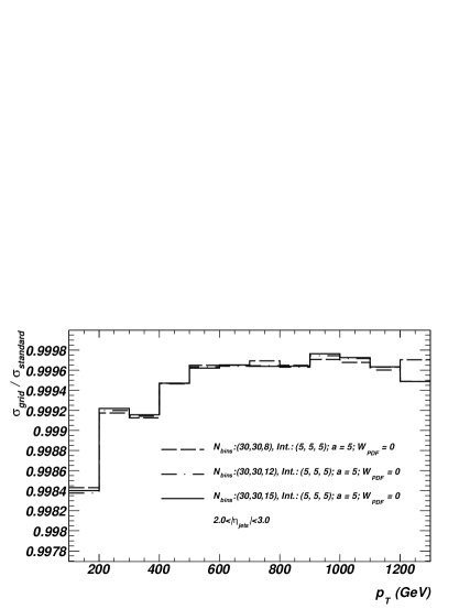
Fig. 4 shows the dependence of the accuracy on the number of -bins. This dependence is rather small. When a large enough number of -bins is chosen, no change is observed for to bins in .
The dependence on the interpolation order (as defined in eq. 3) is shown in Fig. 5. While varying the default interpolation order to and gives similar results within , the interpolation order leads to an accuracy loss of at low transverse jet momenta in the central regions, and by at low and high transverse jet momenta in the forward region.
In conclusion, the results in Figs. 2-5 demonstrate that an accuracy of % can be reached with a reasonable weight grid size. The most critical parameter is the number of -bins, which must be large enough to accommodate strong PDF variations in certain phase space regions. In comparison, the dependence on the number of bins is rather weak. The interpolation between the grid points is sufficiently accurate to allow the grid technique to be used and fifth order interpolation produces reasonable results. The achieved accuracy is probably sufficient for all practical applications.
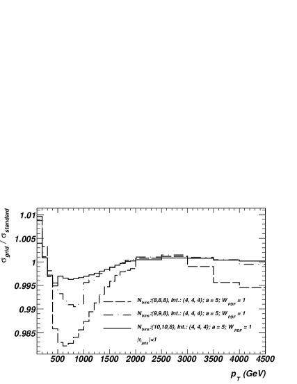
In applications where a very small weight grid is needed, one can also introduce a PDF-weight to flatten out the -dependence of the PDFs (see eq. 17). The PDF weight is calculated using and . This is illustrated in Fig. 6, where grids with very low number of -bins (, , ) and eight bins are used, the interpolation is lowered to . Even with the smallest weight grid an accuracy of is achieved using the PDF-weight. For a somewhat larger weight grid with -bins the accuracy is in all phase space regions.
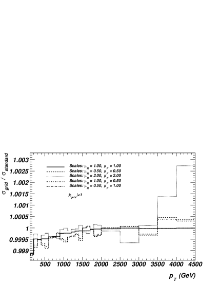
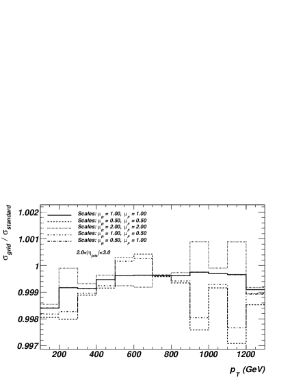
One of the important theoretical uncertainties in NLO QCD calculations is the variation of the results with the choice of the factorisation and renormalisation scale. Eq. 2.5 allows the calculation of the cross-section for any scale choice a posteriori from one weight grid produced at a fixed scale choice. The results from scale variations by a factor of up and down is shown in Fig. 7. The renormalisation and factorisation scales are either varied together or varied individually. The weight grid result has been calculated with a single weight grid and the reference cross-sections have been calculated by repeating the standard NLO QCD calculation for each of the scale variations. The cross-section calculated with the weight grid reproduces the standard results to within about % in the central region and % in the forward region.
4.2 Reweighting jet cross-sections to a different centre-of-mass energy
As outlined in section 2.6 a weight grid produced at a given centre-of-mass energy can also be used to calculate the cross-section at a lower or higher centre-of-mass energy. This procedure works if the coverage in in the weight grid is large enough. For instance, when lowering the centre-of-mass energy to calculate the jet cross-section at a fixed transverse jet momentum, it might happen that the required large values are not present in the weight grid produced at a higher centre-of-mass energy. The variation of the centre-of-mass energy has therefore to be done with care by the user.
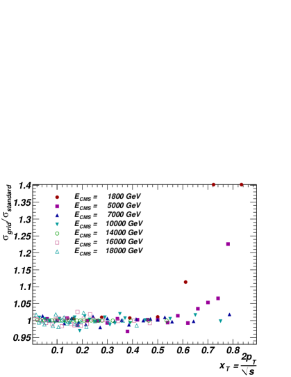
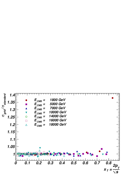
As an example, the accuracy of the jet cross-section calculation using the default weight grid at a fixed centre-of-mass energy of GeV is investigated. Reference cross-sections are calculated at various centre-of-mass energies, i.e. , , , , , and GeV. Since the calculations at the various centre-of-mass energies are statistically independent, each reference cross-section as well as the default weight grid at GeV needs to be calculated with large event samples. Each of the calculations is done with events produced with NLOJET++ .
In order to make the comparisons more meaningful the jet transverse momentum is transformed to . For central jets the variable gives approximately the momentum fraction of the incoming parton with respect to the proton. Fig. 8a) shows the ratio of the cross-section calculated with the standard weight grid produced at GeV to the cross-section calculated at various centre-of-mass energies in the standard way as a function of . For most points, the calculations agree within . The observed fluctuations are statistical.
For large changes in centre-of-mass energy and large values the approximation of the standard grid becomes inaccurate. For instance, for GeV and the weight grid calculation gives a result that is higher than the standard calculation. This discrepancy increases further for large values. The ratio of the last two values becomes very large.121212In Fig. 8a) they are drawn at for better visibility of the rest of the points.
Fig. 8b) shows the result for a larger grid using bins in and bins in . With such a grid the deviations are mostly reduced to statistical fluctuations. Only the largest value for the lowest centre-of-mass energy exhibts a deviation by % from the standard calculation.
A small grid with a PDF weighting leads to large discrepancies to the standard calculation and cannot be used.
In conclusion, the grid technique gives a good accuracy to compute the jet cross-section at various centre-of-mass energies. For very high transverse momenta and extreme centre-of-mass variations a large grid might be required.
4.3 W-boson production at hadron colliders
To further demonstrate the performance of the weight grid method, the production of -bosons at LHC energies is taken as example. The observable that will be examined is the transverse-momentum distribution of the positron from W+-boson decays, when the positron is either central , or very forward, .
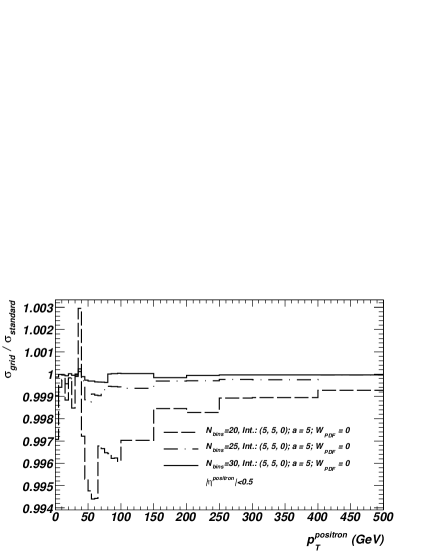
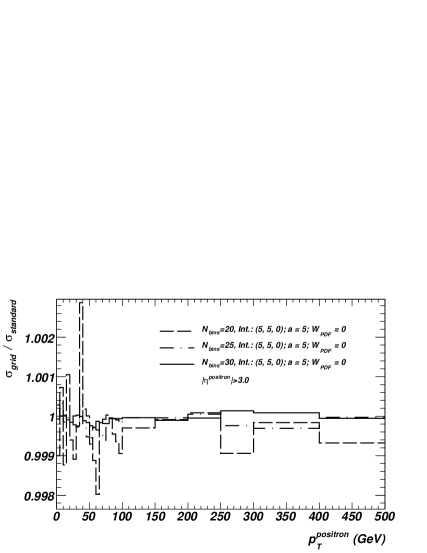
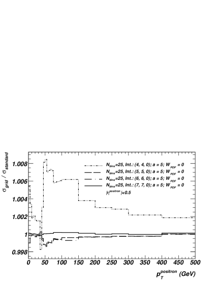

As in the previous section, a default weight grid is defined and variations in a few parameters are studied. The default weight grid consists of bins in . The points are distributed according to eq. 1 with and a fifth order interpolation is used. No PDF weight (see eq. 17) is used. The cross-sections are calculated with the factorisation and renormalisation scale fixed to the mass of the -boson. Therefore, the weight grid need only be two dimensional.
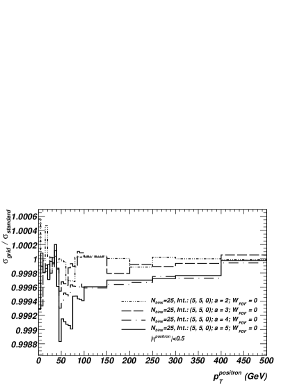
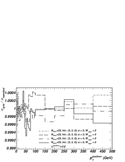
The influence of the number of bins in is shown in Fig. 9. If the number of bins in is too small () the cross-section is reproduced to about in the central region and in the forward region.
For the default weight grid, lowering the interpolation order from to results in an accuracy loss of about over much of the range, as shown in Fig. 10. The accuracy for positrons with low transverse momenta degrades to . The good precision for can only be improved using .
Fig. 11 shows the dependence on the grid spacing parameter corresponding to the parameter in eq. 1. The -values in the cross-section calculation are not large and consequently a fine spacing at large (corresponding to a large parameter) is not needed and the result improves for low values. An accuracy of better than is achieved for all variations.

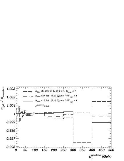
Finally, Fig. 12 shows that, if a PDF weighting is used, it is possible to use very small grid sizes. For a weight grid with only eight -bins an accuracy of can be achieved. In this case the gain in accuracy is small when increasing the number of -bins. Only in the forward region and for high transverse energies the increase in the number of -bins is beneficial.
In summary, a sufficient accuracy is achieved with about -bins and a fifth order interpolation. An equidistant grid spacing () is sufficient.
4.4 CPU and computer memory performance
The execution time for each call to the filling routine for the grid has been studied on a GHz PowerPC and a GHz Intel Xeon running Linux, using a dummy structure with points in each dimension. Fig. 13 shows the performance for various grid architectures. The grids are based on either the ROOT TH3D class, the custom sparse class (SparseMatrix3d) described in the section 3, or the TMatrixDSparse class which implements the 2-dimensional Harwell-Boeing matrix representation. In the latter case, a sparse 1-dimensional structure of TMatrixDSparse matrices using the classes of the SparseMatrix3d has been used to create a sparse 3-dimensional structure.
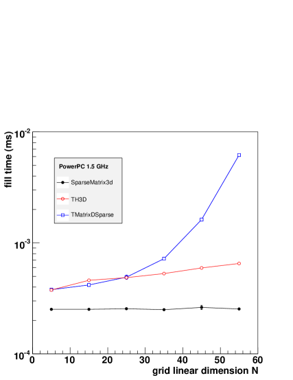
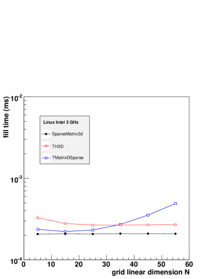
As expected the Harwell-Boeing based class is very quick for filling when the grid is small, but as the grid size becomes larger, since the occupation is reasonably large, the number of entries that must be examined becomes large and the filling time increases rapidly. For the TH3D and custom sparse structures, the filling time is largely independent of the grid size.
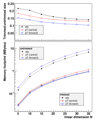
The reduction in memory occupied by the custom sparse grid structure after trimming away unoccupied elements is illustrated in Fig. 14. The bottom-left plot shows the absolute size of the stored elements in MBytes, both before, and after trimming away unfilled elements. The top-left plot shows the fraction of the total, untrimmed grid size, occupied by the filled elements. As the grid spacing decreases, the overall grid size naturally increases.
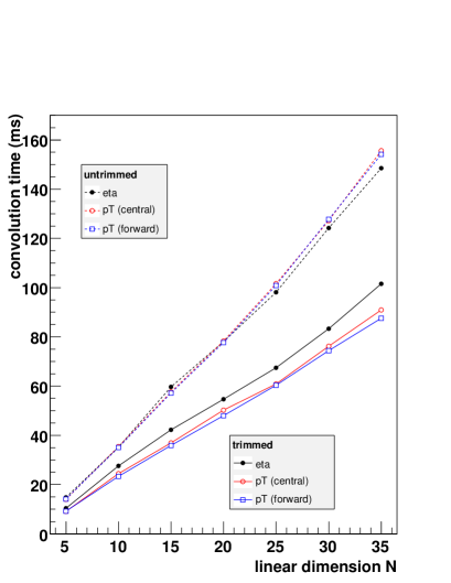
The execution time using the grid to perform the final cross-section calculation including the PDF convolution has also been studied using a 1.5 GHz PowerPC. The results are based on calculations of differential cross-sections with respect to the positron pseudo-rapidity and transverse momentum in -boson production using MCFM [16, 17], as presented in section 4.3. The cross sections involve 20 and 24 bins for the lepton pseudo-rapidity and transverse energy distributions respectively. Fig. 14b shows the convolution time for grids with bins in dimensions and for the sparse structure. Results are given for the trimmed and untrimmed structures In the case of the untrimmed grid, all data elements are retained in the convolution, even those with no entries.
Excluding the unfilled data elements in the convolution improves the convolution time by a factor approaching two. In addition, we see that the convolution time varies approximately linearly with the grid linear dimension. This is because the most costly part of the convolution is the calculation of the PDF at the grid nodes. With independent grid nodes for and , there are evaluations of the PDF for each observable bin, and so the convolution scales linearly with .
In conclusion, the custom sparse structure using trimmed blocks gives the best performance.
5 Application example: Calculation of NLO QCD uncertainty for inclusive jet cross-sections for proton proton collisions at various centre-of-mass energies
As an example in this section the uncertainties of the inclusive jet cross-section in the central region () are evaluated from the default grid obtained at a centre-of-mass energy of GeV. The jet cross-sections are calculated at various centre-of-mass energies. The most recent PDF parameterisations along with their associated uncertainties are used, i.e. CTEQ6.6 [22], MSTW2008 [23], HERAPDF01 [24] and NNPDF [25].
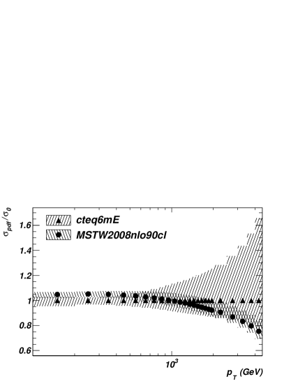
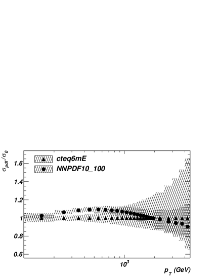
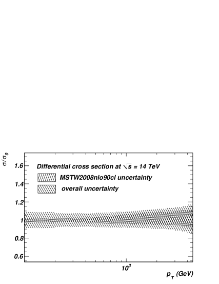
Fig. 15 shows the effect of the PDF uncertainty from CTEQ6.6 (a), MSTW2008 (b), HERAPDF01 (c) and NNPDF (d) on the inclusive jet cross-section with respect to the central value of the somewhat older PDF, CTEQ6mE [18]. The uncertainty from the CTEQ6mE PDF is also overlayed. The band illustrates the result of adding the jet cross-sections obtained for each of the PDF variations131313 The uncertainty band is obtained using eq. 51 and eq. 52 in ref. [23] for the HERA, MSTW and the CTEQ PDFs. This formula has also been suggested earlier in ref. [26]. For the NNPDF eq. 164 in ref. [25] is used. The uncertainty in the NNPDF corresponds to the standard deviation of all variations, while in the case of the other PDFs it corresponds to the 90% confidence limit. For better comparison, the uncertainties of the NNPDF and the HERAPDF01 have been scaled up using eq. in ref. [25]. . The marker indicates the central value. Fig. 16 shows the PDF uncertainty together with the renormalisation and factorisation scale uncertainty added in quadrature with respect to the central value for each of the PDFs.
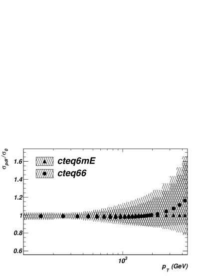

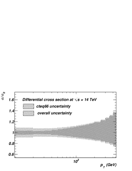
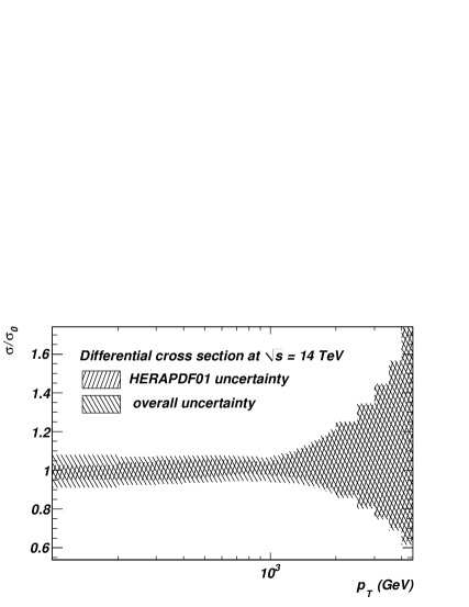
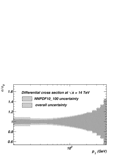
For GeV the jet cross-section obtained with CTEQ6.6 is about smaller than from CTEQ6mE. Above this value the CTEQ6.6 cross-section increases with respect to the one from CTEQ6mE as the jet increases. At GeV it is about equal and at GeV it is about larger. The uncertainty is reduced for the CTEQ6.6 PDF. The uncertainty is about % for GeV, about % at GeV and about % at GeV.
The MSTW2008 PDF gives a jet cross-section that is larger than the one obtained with CTEQ6mE at GeV and is about the same at GeV and then further decreases. The uncertainty is only about % for GeV and then increases to about at GeV. The MSTW2008 PDF gives a smaller uncertainty than the CTEQ6.6 PDF. It seems that the differences between the jet cross-section calculated with CTEQ6.6 and MSTW2008 are a bit larger than the individual uncertainties.
The result obtained with the HERAPDF01 is more similar to the one obtained from MSTW2008 than the one from CTEQ6.6. At low the central value is about higher than the one from CTEQ6mE. In the region GeV the HERAPDF01 predicts a lower jet cross-section than the other PDFs. The uncertainty is about for GeV and then increases to about at GeV. The small uncertainty of the jet cross-section calculated with the HERAPDF01 is remarkable, since only DIS data are used. However, model and parametrization uncertainties are not included in this cross-section calculation. The MSTW and CTEQ sets do not yet include the most recent HERA data. The NNPDF predicts jet cross-sections that are higher than the one from the other PDFs; in particular in the region GeV. The uncertainty is about at low , at GeV and at GeV.
The overall uncertainty, i.e. including the PDF and the scale variation added in quadrature, is shown in Fig. 16. It is about up to a of about GeV and then increases towards higher . It is about % at GeV. For very high the PDF uncertainty dominates.
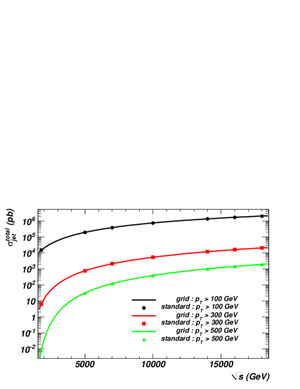
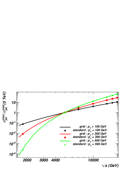

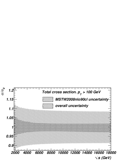
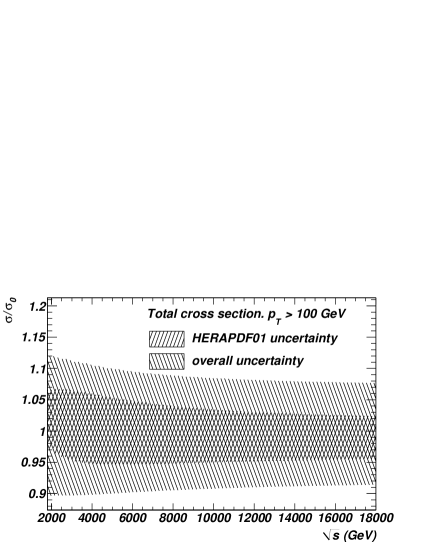
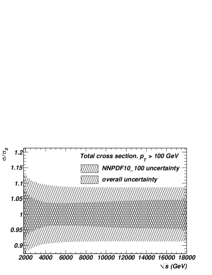
Fig. 17a) shows the total inclusive cross-section for central jets () integrated for GeV, GeV and GeV as a function of the centre-of-mass energy. The markers denote the reference cross-section calculated in the standard way. The lines are obtained from a weight grid produced at GeV. The cross-section calculation from the default weight grid reproduces the reference cross-sections within (see also section 4.2). For each jet transverse momentum threshold the total jet cross-section rises with increasing centre-of-mass energy. Fig. 17b) shows the centre-of-mass energy dependence of the jet cross-section normalised to the jet cross-section at GeV for each jet transverse momentum threshold. As expected the centre-of-mass energy dependence is strongest for high transverse jet momenta.
Fig. 18 shows for each of the considered PDF sets the PDF uncertainty along with the renormalisation and factorisation scale uncertainty added in quadrature for jets with GeV as a function of the centre-of-mass energy . Both the PDF and the scale uncertainties only depend weakly on the centre-of-mass energy. For high centre-of-mass energies the uncertainties are a bit smaller.
6 Application example: PDF fit including DIS data and jet production data at hadron colliders
An important application of the method outlined above, is the consistent inclusion of final state measurements from hadronic colliders into the final extraction of PDFs by NLO QCD fits. Measurements of final states – such as jet production or the production of lepton pairs via the Drell-Yan process – can provide important additional constraints on the proton PDFs, complementary to those from inclusive DIS data.
As a simple “proof-of-principle” example, the grid technique outlined in this paper has been used to include simulated LHC jet data into a NLO QCD fit. The fit framework used here is based on the recent ZEUS-JETS PDF, derived from a fit to inclusive DIS and jet data from HERA. Jet cross-sections from the TEVATRON or any other data than that from HERA are not used. Full details of the data-sets, PDF parameterisation and other assumptions are given elsewhere[5].
To represent the LHC data for inclusion in the fit, jet production from proton-proton collisions at a centre-of-mass energy of GeV was simulated using the JETRAD[27] program, using the CTEQ6.1 PDF[28]. Single inclusive jet cross sections, differential in , were obtained in three regions of rapidity: , and . A grid with default parameters, as described in Sec. 4.1, was produced and interfaced to the ZEUS NLO QCD fit program. Several fits were performed, using different assumptions on the statistical and systematic uncertainties on the simulated data. The PDF uncertainties were calculated using the Hessian method[29, 30], with 141414Note that a using in the Hessian method is generally considered to underestimate the PDF uncertainties. However, the main aim of this study is to provide a proof-of-principle example of the use of the grids discussed in this paper, and not to provide qualitative estimates of weight expected PDF uncertainties. Furthermore, all fits shown in this section have used the same definition of the PDF uncertainties, such that any comparison should still be valid..
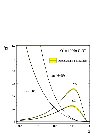
A representative result is shown in Fig. 19. In this example, the statistical uncertainty on the simulated LHC jet data corresponds to an integrated luminosity of and uncorrelated systematic uncertainties have been assumed to be at a level of . A precise jet energy scale uncertainty of (corresponding to on the generated cross-sections) has also been assumed, and is included as a correlated systematic in the fit. Fig. 19 a) shows the up-valence, down-valence, total sea and gluon PDF distributions as a function of , at . The shaded band shows the results of the fit including the simulated LHC jet data. In Fig. 19 b), the fractional uncertainties on the gluon PDF, at a number of values, are shown.
Comparison with the results from a fit which does not include the simulated LHC jet data indicates that some constraint on the high- gluon could be provided by the LHC single inclusive jet data151515Note that the fit without the simulated LHC jet data is not identical to the ZEUS-JETS fit since the standard ZEUS fit[5] uses the Offset method to determine the PDF uncertainties. The ZEUS fit shown here is a modified version of the published analysis, with uncertainties determined using the Hessian method, with . Different treatments of experimental uncertainties in PDF analyses are discussed extensively elsewhere[29, 30, 31, 32].. However, this is reliant on a very precise knowledge of the jet energy scale.
In fact, according to this study, a precise knowledge of the jet energy scale is the key factor. Other fits, which assumed a smaller integrated luminosity ( ) or larger uncorrelated systematics (), still indicated an improvement on the gluon uncertainties, provided the jet energy scale uncertainty was kept at a level of . However, fits in which the latter uncertainty was assumed to be larger, indicated little or no improvement in the gluon uncertainty compared to the reference. More details can be found in ref. [33].
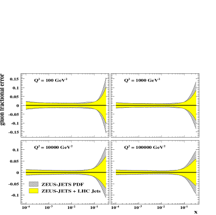
Such precision on the jet energy scale is achievable, but will require a lot of experimental work on the understanding of the LHC detectors. The inclusion of TEVATRON jet cross-sections in the NLO QCD fit might provide further constrains. However, it may be the case that ratios of jet cross sections – for example, in different rapidity regions – may have substantially smaller systematic uncertainties, while retaining sensitivity to the gluon density in the proton. Further constraints on the proton PDFs are also expected from Drell-Yan data measured at LHC or any other data than those from HERA. Such data sets can now be consistently included in NLO QCD fits.
Conclusions
A technique has been developed to store the perturbative coefficients calculated by a NLO QCD Monte Carlo program in a look-up table (grid) allowing for a posteriori inclusion of an arbitrary parton density function (PDF) set and of alternative values of the strong coupling constant as well as for a posteriori variation of the renormalisation and factorisation scale. This extends a technique that has already been successfully used to analyse HERA data to the more demanding case of proton-proton collisions at LHC energies.
The technique can be used to constrain PDF uncertainties by allowing the consistent inclusion of final state observables in global QCD PDF fit analyses. This will help to increase the sensitivity of the LHC to find new physics as deviations from the Standard Model predictions.
An accuracy of better than % can be reached with reasonably small look-up tables for the single inclusive jet cross-section in the central rapidity region , for jet transverse momenta () from to and about for jets in the forward rapidity region . Similar accuracy can be achieved for the differential cross-sections in rapidity and transverse momentum of electrons produced in and -boson decays. This was examined in the central and very forward regions for transverse momentum up to .
The look-up tables provide a powerful tool to quickly evaluate the PDF and scale uncertainties of the cross-section at various centre-of-mass energies. The most recent PDFs predict jet cross-sections in the central rapidity region within a few percent accuracy over a large range of jet transverse momenta.
This technique has been successfully applied to a PDF fit using inclusive deep-inelastic scattering and jet data measured at the electron-proton collider HERA and using simulated LHC jet cross-sections. An improvement on the uncertainty of the gluon density can only be achieved if the jet energy scale is very precisely known. A more comprehensive analysis will be possible in the future, since the grid technique can be applied to most of the available NLO QCD calculations.
Acknowledgements
We would like to thank J. Campbell, T. Kluge, Z. Nagy, K. Rabbertz, T. Schörner-Sadenius, M. H. Seymour, P. Uwer and M. Wobisch for useful discussions on the grid technique and A. Vogt for discussions on moment-space techniques. We thank Z. Nagy for help and support with NLOJET++ and J. Campbell for help and support with MCFM. C. Gwenlan and M. Sutton would like to thank the UK Science and Technology Facilities Council for support. G. P. Salam would like to thank Rutgers University for hospitality while this work was being completed. F. Siegert would like to thank CERN for the Summer Student Program. P. Starovoitov would like to thank for the support given from INTAS. We would also like to thank J. Ribassin for the work he did towards the MCFM interface.
Appendix A: sub-processes for W- and Z-boson production
The production of - and -bosons in proton-proton collisions involves flavour-dependent electro-weak couplings. Therefore, the number of sub-processes that need to be defined is larger than in the case of jet production. To reduce the number of sub-processes as much as possible, quarks are assumed to be massless and the CKM matrix elements [34, 35] to describe the contributions of the various quark flavours are used.
In the case of -boson production combinations of initial state partons need to be distinguished:
| (18) |
where denotes gluons and denotes up (down)-type quarks. Use is made of the generalised PDFs defined as:
| (19) |
where is the PDF of flavour for hadron and () denotes the first or second hadron.
In the case of -boson production161616The case of -boson can be treated in an analogous way. initial state combinations are needed:
| (20) |
where the generalised PDFs are used. They are defined as:
| (21) |
where are the CKM matrix elements.171717 The CKM matrix elements are stored together with the weight grid in the same file. This ensures that the same values are used in the NLO calculation and in the PDF combinations. This choice can be changed a posteriori according to the needs to the user. In MCFM, only four non-zero CKM matrix elements are used.
For simplicity in the former equations we omitted the top contribution, since the parton densities are zero for most practical applications.
Appendix B: Automated identification of sub-processes
In general there are ( flavour) possible PDF combinations for proton proton collisions. In order to store only the minimal amount of information, one needs to establish which of those combinations always come with correlated weights, or equivalently one should identify the underlying physical sub-processes. So far, for each process under study, the sub-processes have been identified manually, on a case-by-case basis. However, the sub-processes can also be found in an automated way.
To simplify the discussion (without loss of generality) it will be convenient to assume that the PDFs are always evaluated at fixed values of . For each event and for each of the PDF combination (with PDF weight ), the NLO QCD program calculates matrix-element weights . The total weight for the event is . The PDF combinations are called channels in the following.
To identify the sub-processes, one determines the weights for events, giving a matrix, whose (event) index labels the rows and whose (PDF channel) index labels the columns. One then carries out an eigenvalue decomposition of the matrix. If denotes the eigenvalue and and the left and right eigenvectors (with components , etc.), then as long as the there are no degenerate eigenvalues, an orthonormality relation can be written:
| (22) |
where the normalisation is our specific choice. Then one can rewrite the matrix as
| (23) |
it being straightforward, for example, to verify that both sides satisfy and . Let us now assume that only of the eigenvalues are non-zero.181818This contradicts the requirement that the eigenvalues be non-degenerate. In practice the rounding errors in the original calculation of the cause the nominally zero eigenvalues to be slightly non-zero, thus alleviating this issue in practice. Then eq. 23 can be interpreted as follows: there are relevant sub-processes; each corresponds to a sub-process that multiplies a linear combination of PDF channels in which the contribution of channel is . In event , sub-process comes with a weight . It will be convenient to denote this by . By virtue of the orthornormality condition eq. 22, we have that , i.e. to determine the weight of sub-process (whose PDF channel combination is given by the left eigenvector ) we take the right-eigenvector that corresponds to this channel and use it to right-multiply the full weight matrix, so to as to eliminate all but the contribution to the sub-process.
The next step is to observe that the sub-processes determined for the first 169 events should hold for all remaining events.191919This is guaranteed as long as the NLO Monte Carlo weights include all sub-processes for each of the first 169 events. So now for any event , we can determine the weight for sub-process , , using the determined from the initial events. Having stored the one can then subsequently reconstruct the full as .
We have verified, in the context of a number of MCFM processes, that this approach is viable in practice202020For carrying out this step in practice, we found the ALGLIB library to be useful, because it provides the necessary software tools written in C++ and has the option of using the mpfr multiple-precision library (available on most distributions), which turned out to be necessary in order to get numerically convergent results for the full set of flavours. The ALGLIB algorithms are translations of the LAPACK ones. . However, it is has yet to be fully integrated with the rest of our grid code and the results shown above are based on the manual sub-process decompositions explicitly spelled out in sections 2.4.1 and in the Appendix A.
One should be aware that while the automated suprocess decomposition yields a number of subprocesses that is identical to what can be found with manual decomposition, the specific linear combinations of PDF channels are usually different. To help understand why, one can take the example of jet production with the 7 subprocesses of eq. 2.4.1. There, rather than using and channels, one might have chosen instead to store weights for the combinations of and channels. More generally, one would have been free to base the grid on any 7 linearly independent combinations of the channels of eq. 2.4.1. For the automated channel decomposition process, the particular independent linear combinations that emerge depend on the random weights of the events used to identify the channels.
References
- [1] D. Graudenz, M. Hampel, A. Vogt and C. Berger, Z. Phys. C 70 (1996) 77
- [2] D. A. Kosower, Nucl. Phys. B 520 (1998) 263
- [3] M. Stratmann and W. Vogelsang, Phys. Rev. D 64 (2001) 114007
- [4] M. Wobisch, Internal Report PITHA 00/12 and DESY-THESIS-2000-049, PhD-thesis RWTH Aachen, 2000
- [5] S. Chekanov et al., (ZEUS Collab.), Eur. Phys. J. C 42 (2005) 1
- [6] P. G. Ratcliffe, Phys. Rev. D 63 (2001) 116004
- [7] M. Dasgupta and G. P. Salam, Eur. Phys. J. C 24 (2002) 213
- [8] G. P. Salam and J. Rojo, Comput. Phys. Commun. 180 (2009) 120
- [9] T. Carli, G. P. Salam and F. Siegert, Contributed to HERA and the LHC: A Workshop on the Implications of HERA for LHC Physics, Geneva (Switzerland); hep-ph/0510324 (2005)
- [10] T. Kluge, K. Rabbertz and M. Wobisch, Proceedings of the DIS 2006 conference, Tsukuba (Japan); hep-ph/0609285 (2006)
- [11] A. Banfi, G. P. Salam and G. Zanderighi, JHEP 07 (2007) 026
- [12] S. Eidelman et al., Phys. Lett. B 592 (2004) 1
- [13] Z. Nagy, Phys. Rev. D 68 (2003) 094002
- [14] Z. Nagy, Phys. Rev. Lett. 88 (2002) 122003
- [15] Z. Nagy and Z. Trocsanyi, Phys. Rev. Lett. 87 (2001) 082001
- [16] J. M. Campbell and R. K. Ellis, Phys. Rev. D 60 (1999) 113006
- [17] J. M. Campbell and R. K. Ellis, Phys. Rev. D 62 (2000) 114012
- [18] J. Pumplin et al. (CTEQ Collab.), JHEP 07 (2002) 012
- [19] G. C. Blazey et al., hep-ex/0005012 (2000)
- [20] G. P. Salam and G. Soyez, JHEP 0705 (2007) 086
- [21] M. Cacciari, G. P. Salam and G. Soyez, JHEP 0804 (2008) 005
- [22] P. M. Nadolsky et al., (CTEQ Collab.), Phys. Rev. D78 (2008) 013004
- [23] A. D. Martin, W. J Stirling, R. S. Thorne and G. Watt, Eur. Phys. J. C63 (2009) 189–285
- [24] H1 and ZEUS collaborations, H1prelim-08-045; ZEUS-prel-08-003 (2008)
- [25] R. Ball et al., Nucl. Phys. B 809 (2009) 1–63
- [26] J. M. Campbell and J. W. Huston and W. J. Stirling, Rept. Prog. Phys. 70 (2007) 89
- [27] W. T. Giele, E. W. N. Glover and D. A. Kosower, Nucl. Phys. B 403 (1993) 633
- [28] D. Stump et al., (CTEQ Collab.), JHEP 0310 (2003) 046
- [29] M. Botje, J. Phys. G 28 (2002) 779
- [30] S. I. Alekhin, IHEP-2000-17 and hep-ex/000504 (2000)
- [31] A.M. Cooper-Sarkar, J. Phys. G 28 (2002) 2609
- [32] R.S. Thorne et al., J. Phys. G 28 (2002) 2717
- [33] A.M. Cooper-Sarkar, Proceedings of the DIS 2007 conference, Munich (Germany); hep-ph/0707.1593 (2007)
- [34] M. Kobayashi and T. Maskawa, Prog. Theor. Phys. 49 (1973) 652
- [35] N. Cabibbo, Phys. Rev. Lett. 10 (1963) 531.