Computing the Bayes Factor from a Markov chain Monte Carlo Simulation of the Posterior Distribution

Abstract

Computation of the marginal likelihood from a simulated posterior distribution is central to Bayesian model selection but is computationally difficult. The often-used harmonic mean approximation uses the posterior directly but is unstably sensitive to samples with anomalously small values of the likelihood. The Laplace approximation is stable but makes strong, and often inappropriate, assumptions about the shape of the posterior distribution. It is useful, but not general. We need algorithms that apply to general distributions, like the harmonic mean approximation, but do not suffer from convergence and instability issues. Here, I argue that the marginal likelihood can be reliably computed from a posterior sample by careful attention to the numerics of the probability integral. Posing the expression for the marginal likelihood as a Lebesgue integral, we may convert the harmonic mean approximation from a sample statistic to a quadrature rule. As a quadrature, the harmonic mean approximation suffers from enormous truncation error as consequence . This error is a direct consequence of poor coverage of the sample space; the posterior sample required for accurate computation of the marginal likelihood is much larger than that required to characterize the posterior distribution when using the harmonic mean approximation. In addition, I demonstrate that the integral expression for the harmonic-mean approximation converges slowly at best for high-dimensional problems with uninformative prior distributions. These observations lead to two computationally-modest families of quadrature algorithms that use the full generality sample posterior but without the instability. The first algorithm automatically eliminates the part of the sample that contributes large truncation error. The second algorithm uses the posterior sample to assign probability to a partition of the sample space and performs the marginal likelihood integral directly. This eliminates convergence issues. The first algorithm is analogous to standard quadrature but can only be applied for convergent problems. The second is a hybrid of cubature: it uses the posterior to discover and tessellate the subset of that sample space was explored and uses quantiles to compute a representative field value. Qualitatively, the first algorithm improves the harmonic mean approximation using numerical analysis, and the second algorithm is an adaptive version of the Laplace approximation. Neither algorithm makes strong assumptions about the shape of the posterior distribution and neither is sensitive to outliers. Based on numerical tests, we recommend a combined application of both algorithms as consistency check to achieve a reliable estimate of the marginal likelihood from a simulated posterior distribution.

Keywords: Bayesian computation, marginal likelihood, algorithm, Bayes factors, model selection

1 Introduction

A Bayesian data analysis specifies joint probability distributions to describe the relationship between the prior information, the model or hypotheses, and the data. Using Bayes theorem, the posterior distribution is uniquely determined from the conditional probability distribution of the unknowns given the observed data. The posterior probability is usually stated as follows:

$$P(\boldsymbol{\theta}|{\cal M},{\bf D})=\frac{\pi(\boldsymbol{\theta}|{\cal M})L({\bf D}|\boldsymbol{\theta},{\cal M})}{Z}$$ (1)

where

$$Z\equiv P({\bf D}|{\cal M})=\int d\boldsymbol{\theta}\,\pi(\boldsymbol{\theta}|{\cal M})L({\bf D}|\boldsymbol{\theta},{\cal M})$$ (2)

is the marginal likelihood. The symbol ${\cal M}$ denotes the assumption of a particular model and the parameter vector $\boldsymbol{\theta}\in\Omega$. For physical models, the sample space $\Omega$ is most often a continuous space. In words, equation (1) says: the probability of the model parameters given the data and the model is proportional to the prior probability of the model parameters and the probability of the data given the model parameters. The posterior may be used, for example, to infer the distribution of model parameters or to discriminate between competing hypotheses or models. The latter is particularly valuable given the wide variety of astronomical problems where diverse hypotheses describing heterogeneous physical systems is the norm (see Gelman et al.,, 2003, for a thorough discussion of Bayesian data analysis).

For parameter estimation, one often considers $P({\bf D}|{\cal M})$ to be an uninteresting normalization constant. However, equation (2) clearly admits a meaningful interpretation: it is the support or evidence for a model given the data. This see this, assume that the prior probability of some model, ${\cal M}_{j}$ say, is $P({\cal M}_{j})$. Then by Bayes theorem, the probability of the model given the data is $P({\cal M}_{j}|{\bf D})=P({\cal M}_{j})P({\bf D}|{\cal M}_{j})/P({\bf D})$. The posterior odds of Model $j=0$ relative to Model $j=1$ is then:

$$\frac{P({\cal M}_{0}|{\bf D})}{P({\cal M}_{1}|{\bf D})}=\frac{P({\cal M}_{0})}{P({\cal M}_{1})}\frac{P({\bf D}|{\cal M}_{0})}{P({\bf D}|{\cal M}_{1})}.$$

If we have information about the ratio of prior odds, $P({\cal M}_{0})/P({\cal M}_{1})$, we should use it, but more often than not our lack of knowledge forces a choice of $P({\cal M}_{0})/P({\cal M}_{1})=1$. Then, we estimate the relative probability of the models given ${\bf D}$ over their prior odds by the Bayes factor $P({\bf D}|{\cal M}_{0})/P({\bf D}|{\cal M}_{1})$ (see Lavine and Schervish,, 1999, for a discussion of additional concerns). When there is no ambiguity, we will omit the explicit dependence on ${\cal M}$ of the prior distribution, likelihood function, and marginal likelihood for notational convenience.

The Bayes factor has a number of attractive advantages for model selection (Kass and Raftery,, 1995): (1) it is a consistent selector; that is, the ratio will increasingly favor the true model in the limit of large data; (2) Bayes factors act as an Occam’s razor, preferring the simpler model if the “fits” are similar; and (3) Bayes factors do not require the models to be nested in any way; that is, the models and their parameters need not be equivalent in any limit. There is a catch: direct computation of the marginal likelihood (eq. 2) is intractable for most problems of interest. However, recent advances in computing technology together with developments in Markov chain Monte Carlo (MCMC) algorithms have the promise to compute the posterior distribution for problems that have been previously infeasible owing to dimensionality or complexity. The posterior distribution is central to Bayesian inference: it summarizes all of our knowledge about the parameters of our model and is the basis for all subsequent inference and prediction for a given problem. For example, current astronomical datasets are very large, the proposed models may be high-dimensional, and therefore, the posterior sample is expensive to compute. However, once obtained, the posterior sample may be exploited for a wide variety of tasks. Although dimension-switching algorithms, such as reversible-jump MCMC (Green,, 1995) incorporate model selection automatically without need for Bayes factors, these simulations appear slow to converge for some of our real-world applications. Moreover, the marginal likelihood may be used for an endless variety of tests, ex post facto.

Newton and Raftery, (1994) presented a formula for estimating $Z$ from a posterior distribution of parameters. They noted that a MCMC simulation of the posterior selects values of $\boldsymbol{\theta}\in\Omega$ distributed as

$$Z\times P(\boldsymbol{\theta}|{\bf D})=L({\bf D}|\boldsymbol{\theta})\pi(\boldsymbol{\theta})$$

and, therefore,

$$Z\times\int_{\Omega}d\boldsymbol{\theta}\,\frac{P(\boldsymbol{\theta}|{\bf D})}{L({\bf D}|\boldsymbol{\theta})}=\int_{\Omega}d\boldsymbol{\theta}\,\pi(\boldsymbol{\theta})=1$$ (3)

or

$$\frac{1}{Z}=\int_{\Omega}d\boldsymbol{\theta}\,\frac{P(\boldsymbol{\theta}|{\bf D})}{L({\bf D}|\boldsymbol{\theta})}=E\left[\frac{1}{L(\boldsymbol{\theta}|{\bf D})}\right]_{P(\boldsymbol{\theta}|{\bf D})},$$ (4)

having suppressed the explicit dependence on ${\cal M}$ for notational clarity. This latter equation says that the marginal likelihood is the harmonic mean of the likelihood with respect to the posterior distribution. It follows that the harmonic mean computed from a sampled posterior distribution is an estimator for the marginal likelihood, e.g.:

$${\tilde{Z}}=\left[\frac{1}{N}\sum_{i=1}^{N}\frac{1}{L({\bf D}|\theta_{i})}\right]^{-1}.$$ (5)

Unfortunately, this estimator is prone to domination by a few outlying terms with abnormally small values of $L_{j}$ (e.g. see Raftery et al.,, 2007, and references therein). Wolpert, (2002) describes convergence criteria for equation (5) and Chib and Jeliazkov, (2001) present augmented approaches with error estimates.

Alternative approaches to computing the marginal likelihood from the posterior distribution have been described at length by Kass and Raftery, (1995). Of these, the Laplace approximation, which approximates the posterior distribution by a multidimensional Gaussian distribution and uses this approximation to compute equation (2) directly, is the most widely used. This seems to be favored over equation (29) because of the problem with outliers and hence because of convergence and stability. In many cases, however, the Laplace approximation is far from adequate in two ways. First, one must identify all the dominant modes, and second, modes may not be well-represented by a multidimensional Gaussian distribution for problems of practical interest, although many promising improvements have been suggested (e.g. DiCicio et al.,, 1997). Trotta, (2007) explored the use of the Savage-Dickey density ratio for cosmological model selection (see also Trotta,, 2008, for a full review of the model selection problem for cosmology).

Finally, we may consider evaluation of equation (2) directly. The MCMC simulation samples the posterior distribution by design, and therefore, can be used to construct volume elements in $k$-dimensional parameter space, $d\boldsymbol{\theta}$, e.g. when $\Omega\subset\mathbb{R}^{k}$. Although the volume will be sparsely sampled in regions of relatively low likelihood, these same volumes will make little contribution to equation (2). The often-used approach from computational geometry, Delaney triangulation, maximizes the minimum angle of the facets and thereby yields the “roundest” volumes. Unfortunately, the standard procedure scales as ${\cal O}(kN^{2})$ for a sample of $N$ points. This can be reduced to ${\cal O}(N\log N+N^{k/2})$ using the flip algorithm with iterative construction (Edelsbrunner and Shah,, 1966) but this scaling is prohibitive for large $N$ and $k$ typical of many problems. Rather, in this paper, we consider the less optimal but tractable kd-tree for space partitioning.

In part, the difficulty in computing the marginal likelihood from the sampled posterior has recently led Skilling, (2006, “nesting sampling”) to suggest an algorithm to simulate the marginal likelihood rather than the posterior distribution. This idea has been adopted and extended by cosmological modelers (Mukherjee et al.,, 2006; Feroz and Hobson,, 2008). The core idea of nesting sampling follows by rewriting equation (3) as a double integral and swapping the order of integration, e.g.

$$Z=\int_{\Omega}d\theta\pi(\theta)\int_{0}^{L({\bf D}|\theta)}dy=\int_{0}^{\sup\{L({\bf D}|\theta):\theta\in\Omega\}}dy\int_{L({\bf D}|\theta)>y}d\theta\pi(\theta).$$ (6)

The nested sampler is a Monte Carlo sampler for the likelihood function $L$ with respect to the prior distrbution $\pi$ so that $L>y$. The generalization of the construction in equation (6) for general distributions and multiple dimensions is the Lebesgue integral (see §2). Clearly, this procedure has no problems with outliers with small values of $L({\bf D}|\boldsymbol{\theta})$. Of course, any algorithm implementing nested sampling must still thoroughly sample the multidimensional posterior distribution and so retains all of the intendant difficulties that MCMC has been designed to solve.

In many ways, the derivation of the nested sampler bears a strong resemblance to the derivation of the harmonic mean but without any obvious numerical difficulty. This led me to a careful study of equations (2) and (3) to see if the divergence for small value of likelihood could be addressed. Indeed they can, and the following sections describe two algorithms based on each of these equations. These new algorithms retain the main advantage of the harmonic mean approximation (HMA): direct incorporation of the sampled posterior without any assumption of a functional form. In this sense, they are fully and automatically adaptive to any degree multimodality given a sufficiently large sample. We begin in §2 with a background discussion of Lebesgue integration applied to probability distributions and Monte Carlo (MC) estimates. We apply this in §3 to the marginal likelihood computation. This development both illuminates the arbitrariness in the HMA from the numerical standpoint and leads to an improved approach outlined in §4. In short, the proposed approach is motivated by methods of numerical quadrature rather than sample statistics. Examples in §5 compare the application of the new algorithms to the HMA and the Laplace approximation. The overall results are discussed and summarized in §6.

2 Integration on a random mesh

Figure 1: Illustration of the integral $\int^{b}_{a}dx\,f(x)$ using Riemann and Lebesgue integration. For Riemann integration, we sum thin vertical rectangles of height $f(X)$ about the abscissa point $X$ for some width $dx$. For Lebesgue integration, we sum thin horizontal rectangles of width $M(Y)$ about the ordinate point $Y$ of height $dy$. In both cases, we sum the area under the curve $f(x)$. In the Lebesgue case, we must add in the rectangle of width $M(y_{0})$ and height $y_{0}$.

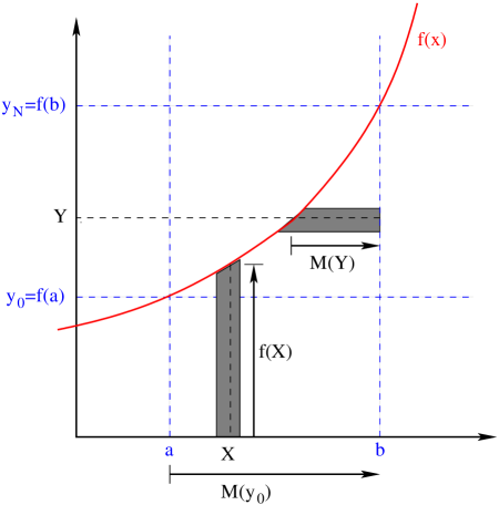
Assume that we have a MC generated sample of random variates with density $f(x)$. Recall that any moment or expectation with respect to this density may be computed as a single sum, independent of the parameter-space dimension! This powerful and seemingly innocuous property follows from the power of Lebesgue integration (e.g. Capinski and Kopp,, 2007). To see this, let us begin by considering a one-dimensional integral

$$I=\int^{b}_{a}f(x)\,dx$$ (7)

where $f(x)$ is non-negative, finite and bounded, that is: $0\leq y_{0}\leq f(x)\leq y_{N}$ for $x\in[a,b]$. More formally, we may define the Lebesgue integral $I$ over the measure of sets of points $x\in\Omega=[a,b]$ with measure $\mu$ as follows. We assume that $f(x)$ is measurable over $\Omega$ and, following Temple, (1971, §8.3), define the measure function $M(y)=\mu(x|f(x)>y)$. Clearly, $M(y)$ is monotonic with $0=M(y_{N})\leq M(y)\leq M(y_{0})$ and $\mu(\Omega)=b-a$. Let ${\cal S}:a\leq x_{0}<x_{1}<\cdots<x_{N}\leq b$ be a partition of $[a,b]$ with $\lim_{N\rightarrow\infty}x_{0}=a$ and $\lim_{N\rightarrow\infty}x_{N}=b$. In our case, the partition ${\cal S}$ is our MC sample. The choice of ${\cal S}$ induces a partition of $y$ through $y_{j}=f(x_{j})$ although the sequence in $y$ will no longer be monotonic. For convenience, reorder the $y$ such that $y_{i-1}\leq y_{i}$. Now consider the Lebesgue integral of $f(x)$ over $\Omega$,

$$I=\int^{b}_{a}f(x)\,dx=\int_{f^{-1}(y)\in\Omega}M(y)\,dy.$$ (8)

We interpret this geometrically as the area under the curve $x=f^{-1}(y)$; in other words, we have swapped the abscissa and ordinate. To see this, define

$${\cal L}_{{\cal S}}=\sum_{i=1}^{N}M(y_{i-1})(y_{i}-y_{i-1})\quad\mbox{and}\quad{\cal U}_{{\cal S}}=\sum_{i=1}^{N}M(y_{i})(y_{i}-y_{i-1})$$ (9)

for the partition ${\cal S}$. Define the interval $\lambda_{i}\equiv y_{i}-y_{i-1}$. Clearly

$${\cal U}_{{\cal S}}-{\cal L}_{{\cal S}}\leq\sum_{i=1}^{N}\left[M(y_{i})-M(y_{i-1})\right]\sup(\lambda_{j})=\left[M(b)-M(a)\right]\sup(\lambda_{j})$$ (10)

and, therefore, $\lim_{N\rightarrow\infty}({\cal U}_{{\cal S}}-{\cal L}_{{\cal S}})\rightarrow 0$ since $M(y)$ is monotonic and $\lim_{N\rightarrow\infty}\lambda_{j}\rightarrow 0$. Using this, we may evaluate the integral in equation (8) as follows:

$$I=M(y_{0})y_{0}+\lim_{N\rightarrow\infty}{\cal L}_{\cal S}=M(y_{0})y_{0}+\lim_{N\rightarrow\infty}{\cal U}_{\cal S}=M(y_{0})y_{0}+\int_{y_{0}}^{y_{N}}M(y)\,dy.$$ (11)

The sums in equation (9) have the form of a rectangular quadrature of the measure over the range of $f(x)$. This geometry is illustrated in Figure 1. Although the Lebesgue integration theory is general, the equivalence of the one-dimensional integral and equation (11) is easily seen by rewriting equation (7) as a two dimensional integral and changing the order of integration using elementary techniques as follows:

$$I=\int^{b}_{a}f(x)\,dx=\int^{b}_{a}\left\{\int_{0}^{f(x)}dy\right\}dx=M(y_{0})y_{0}+\int^{f_{max}}_{f_{min}}M(y)dy$$

where $f_{min}$ and $f_{max}$ are the minimum and maximum values of $f(x)$ in $[a,b]$.

An average of the sums in equation (9) gives us a trapezoidal rule analog:

$${\cal T}_{{\cal S}}=\frac{1}{2}\sum_{i=1}^{N}\left[M(y_{i-1})+M(y_{i})\right](y_{i}-y_{i-1}).$$ (12)

Further generalization is supported by the Lebesgue theory of differentiation. A central result of the theory is that a continuous, monotonic function in some interval is differentiable almost everywhere in the interval (Temple,, 1971). This applies to the measure function $M(Y)$. This result may be intuitively motivated in the context of our marginal likelihood calculation as follows. Our measure function describes the amount of density with likelihood smaller than some particular value. A typical likelihood surface for a physical model is smooth, continuous, and typically consists of several discrete modes. Consider constructing $M(Y)$ by increasing the value of $Y$ beginning at the point of maximum likelihood peak. Since $Y=L^{-1}$, this is equivalent to beginning at $\max(L)=Y^{-1}_{0}$ and decreasing $L$. Recall that $M(Y)$ decreases from 1 to 0 as $Y$ increases from $Y_{0}$ to $\infty$. Therefore, we construct $M(Y)$ from $M(Y+\Delta Y)$ by finding the level set corresponding to some value of $Y$ and subtracting off the area of the likelihood surface constructed from the perimeter of the set times $\Delta Y$. The function $M(Y)$ will decrease smoothly from unity at $Y_{0}$ until $Y$ reaches the peak of the second mode. At this point, there may be a discontinuity in the derivative of $M(Y)$ as another piece of perimeter joins the level set, but it will be smooth thereafter until the peak of the third mode is reached, and so on. Since we expect the contribution to $Z$ to be dominated by a few primary modes, this suggests that we can evaluate the integral $I$ numerically using the quadrature implied by equation (11) and possibly even higher-order quadrature rules. These arguments further suggest that partitioning $\Omega$ into separate domains supporting individual modes would improve the numerics by removing discontinuities in the derivative of $M(Y)$ and explicitly permitting the use of higher-order quadrature rules. This partition may be difficult to construct automatically, however.

To better control the truncation error for this quadrature, we might like to choose a uniform partition in $y$, $\lambda=\lambda_{i}$, to evaluate the sums ${\cal L}_{N}$ and ${\cal U}_{N}$. For MC integration, this is not possible. Rather, MC selects ${\cal S}$ with irregular spacings and this induces a partition of $y$. Motivated by kernel density estimation, we may then approximate $M(y)$ by

$${\tilde{M}}(y)=\frac{1}{N}\sum_{j=0}^{N}\Theta_{j}(y)$$ (13)

where $\Theta(\cdot)$ monotonically increases from 0 to 1 in the vicinity of $f(x_{j})$. For example, we may choose $\Theta$ to be the Heaviside function

$$\Theta_{j}(y)=\begin{cases}1&y<f(x_{j})\quad\mbox{or}\quad y\leq f(x_{j}),\\ 0&\mbox{otherwise}\end{cases}$$ (14)

which assigns a “step” to the upper value of the range in $y$ for each $x_{j}$. Alternatively, we may consider smoothing functions such as

$$\Theta_{j}(y)=\frac{1}{2}\left[1+\operatorname{erf}\left(\frac{y-f(x_{j})}{\alpha_{j}}\right)\right]$$ (15)

where $\operatorname{erf}(\cdot)$ denotes the error function. Then, upon substituting equation (13) into equation (11) for ${\cal U}_{\cal S}$, we get:

$${\tilde{I}}_{N}=M(y_{0})y_{0}+\sum_{j=1}^{N}M(y_{j-1})(y_{j}-y_{j-1})=\sum_{j=1}^{N}\mu_{j}f(x_{j})$$ (16)

where $\mu_{j}={\tilde{M}}(y_{i-1})-{\tilde{M}}(y_{i})$ and ${\tilde{M}}(y_{N})=0$ by construction and the final equality follows by gathering common factors of $y_{i}=f(x_{i})$ in the earlier summation.

For integration over probability distributions, we desire $x$ distributed according some probability density $g(x)$,

$$I[f]=\int_{\mathbb{R}}f(x)g(x)\,dx,$$ (17)

which yields

$$M(y)=\int_{f(x)>y}g(x)\,dx$$ (18)

with the normalization $\int g(x)\,dx=1$, and therefore, $M(y)\in[0,1]$. Despite the appearance of the density $g$ in equation (17), only the value of measure has changed, not the formalism, i.e. the points $x_{j}$ are now sampled from $g(x)$ rather than uniformly.

Let us now consider the connection between equation (16) and a classic MC integration, although we do not need this for later sections of this paper. For a classic MC integration, we choose $\mu_{j}=\mu(\Omega)/N=\mbox{constant}$ by construction, and with this substitution ${\tilde{I}}$ becomes the MC approximation:

$${\tilde{I}}_{N}^{MC}=\frac{b-a}{N}\sum_{j=1}^{N}f(x_{j}).$$

For integration over probability distributions, we assign $\mu_{j}$ to its expectation value $\mu_{j}=1/N$ and the MC integral becomes

$${\tilde{I}}_{N}^{MC}=\frac{1}{N}\sum_{j=1}^{N}f(x_{j}),$$ (19)

although intuition suggests that the explicit form from equation (16) will yield a better result.

The development leading to equation (16) remains nearly unchanged for a multidimensional integral:

$$I=\int_{\mathbb{R}^{k}}f(\boldsymbol{x})g(\boldsymbol{x})d^{k}x.$$ (20)

As in the one-dimensional case, the Lebesgue integral becomes

$$I = \int_{\mathbb{R}^{k}}f(\boldsymbol{x})g(\boldsymbol{x})\,d^{k}x$$ (21)

$$= M(y_{0})y_{0}+\lim_{N\rightarrow\infty}{\cal L}_{{\cal S}}=M(y_{0})y_{0}+\lim_{N\rightarrow\infty}{\cal U}_{{\cal S}}$$

$$= M(y_{0})y_{0}+\int_{y_{0}}^{y_{N}}M(y)\,dy.$$

where the only difference is that $M(y)$ is now the measure of the set of points with $y\leq f(\boldsymbol{x})$ with $\boldsymbol{x}\in\mathbb{R}^{k}$. Perhaps more remarkable than the similarity of equation (11) with equation (21) is that the numerical Lebesgue integral is one-dimensional independent of the dimensionality $k$. However, this does not simplify the computational work; one still needs to sample a subset of $\mathbb{R}^{k}$ to evaluate equation (21). The MC version proceeds similarly as well: replace $x_{j}$ by ${\bf x}_{j}$ in equation (19).

In summary, Monte Carlo integration is most often posed as the expectation over a distribution, which, more generally, is a Lebesgue integral. Lebesgue integration and differentiation theory suggests alternative computational approaches akin to traditional Riemann-based numerical analysis, if the underlying likelihood function and prior probability density are well-behaved functions. We will see in the next section that a truncation-error criterion applied to the marginal likelihood integral in the form of equation (21) can improve the HMA.

3 Application to the marginal likelihood integral

Now, given a MC-computed sample from the posterior distribution $P(\boldsymbol{\theta}|{\bf D})$ with prior distribution $\pi(\boldsymbol{\theta})$ and likelihood function $L({\bf D}|\boldsymbol{\theta})$, how does one compute the marginal likelihood? The integral in equation (2) states that marginal likelihood is the expectation of the likelihood with respect to the prior distribution. This is the same as equation (21) with $\boldsymbol{\theta}\in\Omega_{s}\subset\mathbb{R}^{k}$ replacing $\boldsymbol{x}$, $L({\bf D}|\boldsymbol{\theta})$ replacing $f(\boldsymbol{x})$, $\pi(\boldsymbol{\theta})$ replacing $g(\boldsymbol{x})$. Alternatively, returning to equation (3), the integral $Z\equiv P({\bf D})$ is implicitly defined by

$$P({\bf D})\int_{\Omega_{s}}\frac{d\boldsymbol{\theta}\,P(\boldsymbol{\theta}|{\bf D})}{L({\bf D}|\boldsymbol{\theta})}=\int_{\Omega_{s}}d\boldsymbol{\theta}\,\pi(\boldsymbol{\theta})\equiv J.$$ (22)

The value $J$ is the probability of $\pi$ over $\Omega_{s}$. We will assume that $\Omega_{s}\subseteq\Omega$; this implies that $J\leq 1$ since $\int_{\Omega}d\boldsymbol{\theta}\pi(\boldsymbol{\theta})=1$. In addition, the existence of equation (22) implies that $L({\bf D}|\boldsymbol{\theta})>0$ almost everywhere in $\Omega$. Defining $Y\equiv L^{-1}$, it follows that the Lebesgue integral of the integral on the left-hand-side of equation (22) is

$$K\equiv\int_{\Omega_{s}}\frac{d\boldsymbol{\theta}\,P(\boldsymbol{\theta}|{\bf D})}{L({\bf D}|\boldsymbol{\theta})}=\int M(Y)\,dY+M(Y_{0})Y_{0}$$ (23)

with measure

$$M(y)=\int_{Y({\bf D}|\boldsymbol{\theta})>y}d\boldsymbol{\theta}\,P(\boldsymbol{\theta}|{\bf D}).$$ (24)

Intuitively, one may interpret this construction as follows: divide up the parameter space $\boldsymbol{\theta}\in\Omega_{s}\subset\mathbb{R}^{k}$ into volume elements sufficiently small that $P(\boldsymbol{\theta}|{\bf D})$ is approximately constant. Then, sort these volume elements by their value of $Y({\bf D}|\boldsymbol{\theta})=L^{-1}({\bf D}|\boldsymbol{\theta})$. The probability element $dM\equiv M(Y+dY)-M(Y)$ is the prior probability of the volume between $Y$ and $Y+dY$.

Clearly $M(Y)\in[0,1]$ and may be trivially computed from a MCMC-generated posterior distribution. Using our finite MC-sampled distributed as the posterior probability, $\boldsymbol{\theta}\sim P(\boldsymbol{\theta}|{\bf D})$, and converting the integral to a sum, we have the following simple estimate for $M_{i}\equiv M(Y_{i})$:

$$M_{i}^{[l]}\equiv\frac{1}{N}\sum_{j=1}^{N}\mathbf{1}_{\{Y_{j}>Y_{i}\}},\qquad M_{i}^{[u]}\equiv\frac{1}{N}\sum_{j=1}^{N}\mathbf{1}_{\{Y_{j}\geq Y_{i}\}},\qquad M_{i}\equiv\frac{M_{i}^{[l]}+M_{i}^{[u]}}{2},$$ (25)

where we have defined the left and right end points from equation (14) and the mean separately so that $M_{i}^{[l]}\leq M_{i}\leq M_{i}^{[u]}$. The indicator function $\mathbf{1}_{\{\}}$ enforces the inclusion of a contribution $1/N$ for index $j$ only if $\{Y_{j}>Y_{i}\}$ or $\{Y_{j}\geq Y_{i}\}$ for the lower and upper form, respectively. Alternatively, these sums may be expressed using equations (13)–(16).

We may now estimate the marginal likelihood from equation (22) using the second part of equation (21) for finite $N$ by gathering terms in $Y_{i}$ to get

$$K \equiv \int M(Y)\,dY+M(Y_{0})Y_{0}$$ (26)

$$\approx {\tilde{K}}\equiv\sum_{i=0}^{N}\left(Y_{i+1}-Y_{i}\right)M_{i}+\frac{M_{0}}{L_{0}}=\sum_{i=0}^{N}\left(\frac{1}{L_{i+1}}-\frac{1}{L_{i}}\right)M_{i}+\frac{M_{0}}{L_{0}}$$ (27)

$$= \sum_{i=1}^{N}\frac{1}{L_{i}}M_{i-1}-\sum_{i=1}^{N}\frac{1}{L_{i}}M_{i}=\sum_{i=1}^{N}\frac{1}{L_{i}}(M_{i-1}-M_{i})=\frac{1}{N}\sum_{i=1}^{N}\frac{1}{L_{i}}.$$ (28)

In deriving equation (28), the leading term $M(Y_{0})Y_{0}$ from equation (21) is absorbed into the sum and $M(Y_{N})=0$. Assuming that $J=1$ in equation (22) and using equation (28) yields

$${\tilde{Z}}\equiv{\tilde{P}}({\bf D})={\tilde{J}}/{\tilde{K}}=\left({\displaystyle\frac{1}{N}\sum_{j}\frac{1}{L_{j}}}\right)^{-1}.$$ (29)

This is an alternative derivation for the “harmonic mean” approximation (HMA) to the marginal likelihood.

3.1 Convergence of $K$

The evaluation of the integral $K$ (eq. 26) may fail both due to insufficient sampling and intrinsic divergence. As an example of the former, a sparse sampling may lead to large intervals $Y_{i+1}-Y_{i}$ and inflated truncation error (eq. 27). We will consider this further in the next section. As an example of the latter, consider the textbook inference of an unknown mean $\theta$ from a sample of $N$ normally distributed points $x\sim{\cal N}(\theta,\sigma_{x}^{2})$. The likelihood function is

$$L(D|\theta)=\prod_{i=1}^{N}\frac{e^{-(x_{i}-\theta)^{2}/2\sigma_{x}^{2}}}{\sqrt{2\pi\sigma_{x}^{2}}}=L_{0}e^{-({\bar{x}}-\theta)^{2}N/2\sigma_{x}^{2}}$$ (30)

where $L_{0}=\sup\{L:x\in\mathbb{R}\}$ and ${\bar{x}}$ is the sample mean. Let the prior distribution for $\theta$ be ${\cal N}(\theta_{0},\sigma_{\theta}^{2})$. We use an MCMC algorithm to sample the posterior distribution $\theta$.

Now, let us evaluate $K$ using Lebesgue integration for this example. To begin, we need the measure function $M(Y)=\int_{L^{-1}(D|\theta)>Y}dP$ with $Y=L^{-1}$ We may use equation (30) to solve for $\theta=\theta(L)$, noting that the solution has two branches. After some algebra, we have:

$$M(Y)=1-\frac{1}{2}\left[\mbox{erf}\left(\frac{{\bar{x}}-{\bar{y}}+\Delta(Y)}{\sqrt{2{\bar{\sigma}^{2}}}}\right)-\mbox{erf}\left(\frac{{\bar{x}}-{\bar{y}}-\Delta(Y)}{\sqrt{2{\bar{\sigma}^{2}}}}\right)\right]$$ (31)

where

$${\bar{y}}\equiv\frac{\sigma_{x}^{2}\theta_{0}/N+\sigma_{\theta}^{2}{\bar{x}}}{\sigma_{x}^{2}/N+\sigma_{\theta}^{2}},\qquad{\bar{\sigma}^{2}}\equiv\frac{\sigma_{\theta}^{2}\sigma_{x}^{2}/N}{\sigma_{x}^{2}/N+\sigma_{\theta}^{2}}=\left(\frac{1}{\sigma_{\theta}^{2}}+\frac{N}{\sigma_{x}^{2}}\right)^{-1},$$

$$Y_{0}\equiv L_{0}^{-1},\qquad\Delta(Y)\equiv\sqrt{\frac{2\sigma_{x}^{2}}{N}\log(Y/Y_{0})}.$$

The value ${\bar{y}}$ is the variance weighted mean of the prior mean and the sample mean, and ${\bar{\sigma}^{2}}$ is the harmonic mean of the variance of the prior distribution and the variance of the sample mean. The value $Y_{0}$ is the minimum value for $Y$ and $\Delta(\cdot)$ describes the offset of $\theta$ with increasing $Y$. Note that $\Delta(Y_{0})=0$.

Since the values of $Y$ are obtained by a sampling, the sample will not cover $[Y_{0},\infty)$ but will be limited from above by the smallest sampled value of the likelihood $Y_{max}=L_{min}^{-1}$. We define this limited value of the Integral $K$ as

$$K(Y_{max}=L_{min}^{-1})\equiv\int_{Y_{0}}^{Y_{max}}dYM(Y)+M(Y_{0})Y_{0}=\int_{Y_{0}}^{Y_{max}}dYM(Y)+Y_{0}$$ (32)

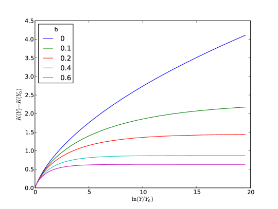
where the last equality uses $M(Y_{0})\equiv 1$. Clearly $K=K(\infty)>K(Y_{max})$. The magnitude of the truncation due to finite sampling, $K(\infty)-K(Y_{max})$, depends critically on the width of the likelihood distribution relative to the prior distribution. We describe this ratio of widths by $b\equiv\sigma_{x}^{2}/(N\sigma_{\theta}^{2})$. The convergence condition $\lim_{Y\rightarrow\infty}[K(\infty)-K(Y_{max})]\rightarrow 0$ requires that $M(Y)$ decreases faster than $Y^{-1-\epsilon}$ for some $\epsilon>0$. For $b=0$ and large $Y$, $\int^{Y}dYM(Y)$ increases as $\log(\log Y)$. For $b>0$, $\int^{Y}dYM(Y)$ decreases at least as fast $Y^{-b}$. Figure 2 shows $K(\infty)-K(Y_{0})$ as a function of $b$ and suggests that $b>0.1$ is sufficient to obtain convergence for practical values of $N$. Qualitatively, a prior distribution that limits $Y$ from above (or, equivalently, $L$ from below) will prevent the divergence.

Figure 2: The integral $K(Y)-K(Y_{0})$ is shown as a function of $Y/Y_{0}$ for various values of the ratio $b\equiv\sigma_{x}^{2}/(N\sigma_{\theta}^{2})$. For an uninformative prior distribution $\sigma_{\theta}\gg\sigma_{x}/N$ and $b\rightarrow 0$ and $K(Y)$ diverges with increasing $Y/Y_{0}$. For an informative prior distribution ${\cal O}(b)\sim 1$ and $K(Y)$ convergences quickly with $Y/Y_{0}$.

Similar asymptotic expressions for $K(Y)$ may be derived for multivariate normal distributions. For simplicity, assume that data is distributed identically in each of $k$ dimensions and, for ease of evaluation, take $\mathbf{\bar{x}}=\mathbf{\bar{y}}$. Then

$$M(Y)=\Gamma\left(\frac{k}{2},(1+b)\log(Y/Y_{0})\right)/\Gamma\left(\frac{k}{2}\right)$$ (33)

where $\Gamma(a,x)$ is the upper incomplete gamma function and $\Gamma(a)$ is the complete gamma function. Using the standard asymptotic formula for $\Gamma(a,x)$ in the limit of large $Y$, one finds that

$$M(Y)\rightarrow\frac{1}{\Gamma(k/2)}\left[\sqrt{1+b^{2}}\log\left(\frac{Y}{Y_{0}}\right)\right]^{k/2-1}\left(\frac{Y}{Y_{0}}\right)^{-1-b}\qquad\mbox{for\ }Y\gg k/2.$$ (34)

This expression reduces to equation (31) when $k=1$, but more importantly, this shows that the tail magnitude of $M(Y)$ increases with dimension $k$. Figure 3 illustrates this for various values of $k$ and $b$.

(a) $b=0.2$

(b) $b=0.6$

Figure 3: As in Figure 2, the integral $K(Y)-K(Y_{0})$ is shown as a function of $Y/Y_{0}$ for the ratio $b=0.2,0.6$ for $k$-dimensional normal data distributions. The integral $K(Y)$ converges more rapidly with increasing $b$ (as in Fig. 2) but increasingly slowly with $k$. The run of $K(Y)-K(Y_{0})$ is normalized to 1 at $Y=\infty$ to facilitate comparison.

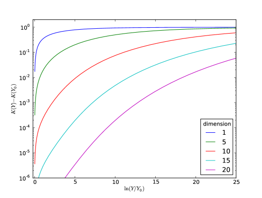
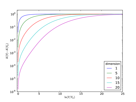
The divergence of $K$ in the limit $\sigma_{\theta}^{2}\rightarrow\infty$ shows that normally distributed likelihood function with an uninformative prior is divergent. Moreover, Figures 2 and 3 further demonstrate that weakly informative prior with very small $b$ is likely to be numerically divergent even if $K$ formally converges. Intuitively, the cause is clear: if the Markov chain never samples the wings of the prior distribution that still make significant contribution to $K$, then $K$ will increase with sample size. Analytically, the failure is caused by the measure decreasing too slowly as $Y$ increases (as described at the beginning of §3). Empirically, the convergence of the integral $K$ may be tested by examining the run of $K(Y)$ for increasing $Y$.

3.2 Application to the MCMC posterior distribution

Overall, §3 highlights the marginal likelihood as a numerical quadrature. We have considered the path of approximations leading from the quadrature to standard expression for the HMA. We have also considered the intrinsic requirements on the prior distribution so that the meausure $M(Y)$ is convergent. This development suggests that there are two sources of error in evaluating equation (22) using equations (23) and (27). The first is a truncation error of order $(Y_{i+1}-Y_{i})^{2}$. The second is a bias error resulting from specifying the computational grid by a Monte Carlo procedure. We will consider each in turn.

Thinking again in terms of numerical quadrature, we can trust the sum in equation (27) when adjacent values of $L_{j}$ are close. The error in ${\tilde{K}}$ will be dominated by the extremely small values of $L_{i}$ that lead to $h_{i}\equiv Y_{i+1}-Y_{i}\gg 1$. Specifically, the error for such a term will be $\propto h_{i}^{2}$, and a small number of such terms can dominate the error for ${\tilde{K}}$. Numerical analysis is based on functional approximation of smooth, continuous, and differentiable functions. This truncation error estimate assumes that $M(Y)$ is such a function. Although not true everywhere, we have argued in §2) that this assumption should be valid over a countable number of intervals in practice. In addition, we expect the sample to be strongly clustered about the value of the posterior mode. By the Central Limit Theorem for a likelihood dominated posterior, the distribution of $\theta$ tends toward a normal distribution. Therefore, larger $N$ will yield more extremal values of $L$ and increase the divergence of $h_{i}=L^{-1}_{i+1}-L^{-1}_{i}$. Eventually, for proper prior distributions and sufficiently large $N$, the smallest possible value of $L$ will be realized as long as $L>0$ (see eq. 22 and following discussion). Further sampling will reduce the largest intervals, and this will lead to the decrease of large $h_{i}$, and finally, convergence.

The second source of error is closely related to the first. After eliminating the divergent samples with $h_{i}\gg 1$, the sampled domain $\Omega_{s}$ will be a subset of the originally defined domain $\Omega_{s}\subset\Omega$. That is, the MCMC sample will not cover all possible values of the parameter vector $\mathbf{\theta}$. This implies that the numerical quadrature of equation (22) will yield ${\tilde{J}}<1$. Identification of these error sources immediately suggests solutions. Note that this observation does not change the problem definition in some new way, but rather, allows us to exploit the MCMC-chosen domain $\Omega_{s}$ to eliminate the divergence for small $b$ described in §3.1.

First, we may decrease the truncation error in ${\tilde{K}}$ by ordering the posterior sample by increasing values of $Y$ and truncating the sequence at the point where $h_{i}>h_{\ast}$ for some choice $h_{\ast}\ll 1$. Next, we need a consistent evaluation for ${\tilde{J}}$. We may use the sampled posterior distribution itself to estimate the sampled volume in $\Omega_{s}\subset\Omega$. This may be done straightforwardly using a space partitioning structure. A computationally efficient structure is a binary space partition (BSP) tree, which divides a region of parameter space into two subregions at each node. The most easily implemented tree of this type for arbitrary dimension is the kd-tree (short for k-dimensional tree). The computational complexity for building the tree from the $N$ sampled points in parameter space scales as ${\cal O}(N\log^{2}N)$ using the Quicksort algorithm at each successive level (this may be improved, see Cormen et al.,, 2001). Each leaf has zero volume. Each non-leaf node has the minimum volume enclosing the points in the node by coordinate planes. Assigning the volume containing a fixed number of leaves ${\bar{m}}$ (e.g. ${\bar{m}}=16$ or $32$), and some representative value of the prior probability in each node (such as a $p$-quantile or mean value), one may immediately sum product of each volume and value to yield an estimate of $J$. For modest values $N$, we will almost certainly find that ${\tilde{J}}<1$. Since the MCMC chain provides the values of $\pi(\boldsymbol{\theta})$ and $P(\theta)=\pi(\boldsymbol{\theta})L({\bf D}|\boldsymbol{\theta})$, we may use the same tree to evaluate both ${\tilde{Z}}$ and ${\tilde{J}}$ over the sampled volume $\Omega_{s}$.

The example in §3.1 suggests that evaluation of $K$ may stymied by poor convergence unless the prior distribution is restrictive. Therefore, if the value of $K$ is divergent or very slowly convergent, the evaluation of $Z$ using $K/J$ will fail whether or not we use the improved truncation criteria. Direct evaluation of the $Z$ is free from this divergence and remains an practical option in this case. The advantage of a direct evaluation is clear: the converged Markov chain samples the domain $\Omega$ proportional to the integrand of equation (2), and therefore, we expect

$$\lim_{N\rightarrow\infty}\int_{\Omega_{s}}d\boldsymbol{\theta}\pi(\boldsymbol{\theta})L({\bf D}|\boldsymbol{\theta})\gg\lim_{N\rightarrow\infty}\int_{\Omega\setminus\Omega_{s}}d\boldsymbol{\theta}\pi(\boldsymbol{\theta})L({\bf D}|\boldsymbol{\theta})\rightarrow 0$$

for large sample size by construction. We propose a hybrid of cubature and Monte Carlo integration. The BSP tree provides a tiling of multidimensional volume by using the posterior distribution to define volume elements, $\Delta V$. We use a $p$-quantile (such as the $p=0.5$ median) or mean value of the posterior probability or the prior probability to assign a probability value to each volume element. An approximation to the integrals $Z$ and $J$ follow from summing the field values over the volume elements, analogous to a multidimensional Riemann rule.

Although $\pi(\boldsymbol{\theta})L({\bf D}|\boldsymbol{\theta})\Delta V=\mbox{constant}$ for a infinite posterior sample, there are several sources of error in practice. First, the variance in the tessellated parameter-space volume will increase with increasing volume and decreasing posterior probability. This variance may be estimated by bootstrap. Secondly, the truncation error of the cubature increases with the number of points per element. As usual, there is a variance–bias trade off choosing the resolution of the tiling: the bias of the probability value estimate increases and the variance decreases as the number of sample points per volume element increases. The prior probability value will be slowing varying over the posterior sample for a typical likelihood-dominated posterior distribution, so the bias will be small. This suggests that larger numbers of points per cell will be better for the evaluation of $J$ and a smaller number will be better for $Z$. Some practical examples suggest that the resulting estimates are not strongly sensitive to the number of points per cell (${\bar{m}}=16$ or 32 appears to be a good compromise). Almost certainly, there will be a bias toward larger volume and therefore larger values of ${\tilde{Z}}$ and this bias will increase with dimension most likely.

To summarize, we have described two approaches for numerically computing $Z$ from a MCMC posterior simulation. The first evaluates of the integral $K$ by numerical Lebesgue integration, and the second evaluates $Z$ directly by a parameter space partition obtained from the sampled posterior distribution. The first is closely related to the HMA. It applies ideas of numerical analysis the integral that defines the HMA. The second is more closely related to the Laplace approximation. In some sense, Laplace approximation is an integral of a parametric fit to the posterior distribution. The tree integration described above is, in essence, an integral of a non-parametric fit to the posterior distribution. The advantage of the first method its amenability to analysis. The disadvantage is the limitation on convergence as illustrated in §3.1. The advantage of the second method is its guaranteed convergence. The disadvantage is its clear, intrinsic bias and variance. The variance could be decreased, presumably, using high-dimensional Voronoi triangulation but not without dramatic computational cost.

3.3 Discussion of previous work on the HMA

The HMA is treated as an expectation value in the literature. One of the failures pointed out by Meng and Wong, (1996) and others is that the HMA is particularly awful when the sample is a single datum. In the context of the numerical arguments here, this is no surprise: one cannot accurately evaluate a quadrature with a single point! Even for larger samples, the HMA is formally unstable in the limit of a thin-tailed likelihood function owing to the divergence of the variance of the HMA. Raftery et al., (2007) address this failure of the statistic directly, proposing methods for stabilizing the harmonic mean estimator by reducing the parameter space to yield heavier-tailed densities. This is a good alternative to the analysis presented here when such stabilization is feasible. As previously mentioned, Wolpert, (2002) presents conditions on the posterior distribution for the consistency of the HMA. Intuitively, there is a duality with the current approach. Trimming the Lebesgue quadrature sum so that the interval $Y_{i+1}-Y_{i}<h_{\ast}$ is equivalent to lopping off the poorly sampled tail of the posterior distribution. This truncation will be one-sided in the estimate of the marginal likelihood ${\tilde{Z}}$ since it removes some of the sample space. However, this may be compensated by an appropriate estimation of ${\tilde{J}}$.

4 The new algorithms

The exposition and development in §3 identifies the culprits in the failure of the HMA: (1) truncation error in the evaluation of the measure $M(Y)$; and (2) the erroneous assumption that $J=1$ when $\Omega_{s}\subset\Omega$ in practice. We now present two new algorithms, the Numerical Lebesgue Algorithm (NLA) and the Volume Tessellation Algorithm (VTA), that implement the strategies described in §3.2 to diagnose and mitigate this error. NLA computes ${\tilde{K}}$ and VTA computes ${\tilde{J}}$ and, optionally, ${\tilde{Z}}$ directly from equation (2). In the following sections, we assume that $\Omega\subset\mathbb{R}^{k}$.

4.1 Description

We begin with a converged MCMC sample from the posterior distribution. After the initial sort in the values of $L_{j}$, the NLA computes the difference $h_{j}=L^{-1}_{j-1}-L^{-1}_{j}$ with $j=N,N-1,\ldots$ to find the first value of $j=n$ satisfying $h_{j}<h_{\ast}$. The algorithm then computes the $M_{i}$ for $i=n,\ldots,N$ using equation (25). For completeness, we compute the $M_{i}$ using both the restriction $L({\bf D}|\boldsymbol{\theta})>L_{i}$ and $L({\bf D}|\boldsymbol{\theta})\geq L_{i}$ to obtain lower and upper estimate for $M(Y)$. Then, these may be combined with ${\cal L}_{S}$ and ${\cal U}_{S}$ from §2 to Riemann-like upper and lower bounds on ${\tilde{K}}$ . See the listing below for details. Excepting the sort, the work required to implement this algorithm is only slightly harder than the HMA.

The VTA uses a kd-tree to partition the $N$ samples from posterior distribution into a spatial regions. These tree algorithms split $\mathbb{R}^{k}$ on planes perpendicular to one of the coordinate system axes. The implementation described here uses the median value along one of axes (a balanced kd-tree). This differs from general BSP trees, in which arbitrary splitting planes can be used. There are, no doubt, better choices for space partitioning such as Voronoi tessellation as previously discussed, but the kd-tree is fast, easy to implement, and published libraries for arbitrary dimensionality are available. Traditionally, every node of a kd-tree, from the root to the leaves, stores a point. In the implementation used here, the points are stored in leaf nodes only, although each splitting plane still goes through one of the points. This choice facilitates the computation of the volume spanned by the points for each node as follows. Let ${\bar{m}}_{j}$ be the number of parameter-space points $\boldsymbol{\theta}^{[n]},n=1,\ldots,{\bar{m}}_{j}$ in the $j^{\mbox{th}}$ node. Let ${\bf f}^{[n]}$ denote the field quantities at each point $\boldsymbol{\theta}^{[n]}$. Some relevant field quantities include the values of the unnormalized posterior probability and the prior probability. The volume for Node $j$ is

$$V_{j}=\prod_{i=1}^{k}\left[\max(\theta^{[1]}_{i},\ldots,\theta^{[{\bar{m}}_{j}]}_{i})-\min(\theta^{[1]}_{i},\ldots,\theta^{[{\bar{m}}_{j}]}_{i})\right].$$ (35)

The set of nodes with ${\bar{m}}={\bar{m}}_{j}=2^{q}$ for some fixed integer $q$, determines an exclusive volume partition of the parameter space spanned by the point set, the frontier. The value of $q$ is chosen large enough to limit the sampling bias of field quantities in the volume but small enough resolve the posterior modes of interest. The values $q\in[2,\ldots,6]$ seem to be good choices for many applications. Each node in the frontier is assigned a representative value ${\bf f}_{\ast}$. I use $p$-quantiles with $p=0.1,0.5,0.9$ for tests here. The resulting estimate of the integrals ${\tilde{J}}$ and/or ${\tilde{Z}}$ follow from summing the product of the frontier volumes with their values ${\bf f}_{\ast}$.

4.2 Performance

Both the NLA and the VTA begin with a sort of the likelihood sequence $L$ and this scales as ${\cal O}(N\log N)$. In the NLA, the computation of the $M_{k}$ followed by the computation of ${\tilde{Z}}$ is ${\cal O}(N)$. The sequence $\{M_{k}\}$ is useful also for diagnosis as we will explore in the next section. However, in many cases, we do not need the individual $M_{i}$ but only need the differential value $M_{i}-M_{i+1}$ to compute ${\tilde{Z}}$, which contains a single term. The values of likelihood may range over many orders of magnitude. Owing to the finite mantissa, the differential value be necessary to achieve adequate precision for large $N$, and the NLA may be modified accordingly. The algorithm computes the lower, upper, and trapezoid-rule sums (eqns. 9–12) for the final integral ${\tilde{Z}}$. For large posterior samples, e.g. $N>10000$, the differences between ${\cal L}_{{\cal S}}$ and ${\cal U}_{{\cal S}}$ are small. Indeed, a more useful error estimate may be obtained by a random partitioning and subsampling of the original sequence $\{L_{k}\}$ to estimate the distribution of ${\tilde{Z}}$ (see the examples in §5). In practice, computing the marginal likelihood from a posterior sample with $N=400000$ takes 0.2 CPU seconds on a single 2Ghz Opteron processor. Although NLA could be easily parallelized over $n$ processors to reduce the total runtime by $1/n$ this seems unnecessary.

The kd-tree construction in VTA scales as ${\cal O}(kN\log^{2}N)$ followed by a tree walk to sum over differential node volumes to obtain the final integral estimates that scales as ${\cal O}(N\log N)$. This scaling was confirmed empirically using the multidimensional example described in §5.3 with dimension $k\in[1,40]$ and sample size $N\in[1000,10000000]$. Computing the marginal likelihood from a posterior sample with $N=400000$ and $k=10$ takes 4.4 CPU seconds on a single 2Ghz Opteron processor, and, therefore, the computation is unlikely to be an analysis bottleneck, even when resampling to produce a variance estimate. The leading coefficient appears to vary quite weakly the distribution, although there may be undiscovered pathological cases that significantly degrade performance. The required value of $N$ increases with parameter dimension $k$; $N=400000$ is barely sufficient for $k=40$ in tests below. Subsampling recommends the use of even larger chains to mitigate dependence of the samples. Therefore, the first practical hardware limitation is likely to be sufficient RAM to keep the data in core.

Algorithm NL. Algorithm to compute the marginal likelihood from a posterior sample by Lebesgue integration. In Line 3, the value of $h_{\ast}$ can be chosen to trim anomalous values of likelihood. In Line 9, both choices for the inequality in $\Theta_{j}$ (see eq. 14) can be computed and stored simultaneously. Combined with Line 18, we can bracket the values by lower and upper sums (algorithmic error).

0:  Likelihood values $\{L_{j}\},j=1,\ldots,N$ from the simulated posterior distribution

1:  Sort the sequence so that $\{L_{j}\geq L_{j-1}\}$

2:  $n=N$ // find the smallest $n$ obeying the threshold condition

3:  while $L_{n-1}^{-1}-L^{-1}_{n}<h_{\ast}$ do

4:     $n\leftarrow n-1$

5:  end while

6:  for $i=n$ to $N$ do

7:     $M_{i}\leftarrow 0$ // compute the measure, see eq. 25

8:     for $j=i$ to $N$ do

9:        $M_{i}\leftarrow M_{i}+1/L_{j}$ and/or $M_{i}\leftarrow M_{i}+1/L_{j+1}$

10:     end for

11:     Save the values $M_{i}$

12:  end for

13:  for $i=n$ to $N$ do

14:     $M_{i}\leftarrow M_{i}/M_{N}$ // normalize the prior measure

15:  end for

16:  ${\tilde{Z}}\leftarrow 0$ // compute the marginal likelihood, see eqns. 9–12

17:  for $i=n$ to $N$ do

18:     ${\tilde{Z}}\leftarrow{\tilde{Z}}+\left(M_{i}-M_{i+1}\right)\left\{\begin{array}[]{ll}L_{i}&\mbox{lower sum}\\ L_{i+1}&\mbox{upper sum}\\ (L_{i}+L_{i+1})/2&\mbox{trapezoidal rule}\\ \end{array}\right\}$

19:  end for

20:  Save the estimated marginal likelihood, ${\tilde{Z}}$ and algorithmic error

Algorithm VT. Algorithm to estimate $J=\int_{\Omega_{s}}d\boldsymbol{\theta}\,\pi(\boldsymbol{\theta}|{\cal M})$ over the domain $\Omega_{s}\subset\Omega$ sampled by the MCMC algorithm using the space partitioning kd-tree.

0:  Likelihood values $\{L_{j}\},j=1,\ldots,N$ from the simulated posterior distribution

1:  Change variables $Y_{j}=1/L_{j}$

2:  Sort the sequence so that $\{Y_{j-1}\leq Y_{j}\}$

3:  Create an empty point set ${\cal P}$

4:  $n\leftarrow 1$ // find the largest $n$ obeying the threshold condition

5:  while $Y_{n+1}-Y_{n}<h_{\ast}$ do

6:     $n\leftarrow n+1$

7:     Add $(\boldsymbol{\theta}^{[n]},{\bf f}^{[n]})$ to ${\cal P}$

8:  end while

9:  $\mbox{Node}_{root}=\mbox{BuildKD}({\cal P})$

10:  Find the set of frontier nodes ${\cal F}$ with the desired number of points ${\bar{m}}$

11:  ${\tilde{G}}\leftarrow 0$

12:  for each node $j\in{\cal F}$ do

13:     Compute the median value of ${\bf f}^{[n]}$ among the ${\bar{m}}$ points

14:     ${\tilde{G}}\leftarrow{\tilde{G}}+V_{j}\times\mbox{median}({\bf f})$

15:  end for

16:  Save the estimated value of the integrals ${\tilde{G}}$

Procedure: BuildKD(${\cal P}$)

0:  A set posterior points and values $(\boldsymbol{\theta}^{[n]},{\bf f}^{[n]})\in{\cal P}$

1:  if ${\cal P}$ contains only one member then

2:     return  pointer to this leaf

3:  else

4:     Compute and store the range for each coordinate and the volume for this node

5:     Locate the coordinate dimension $j\in 1\ldots k$ with maximum variance

6:     Determine the median value of $\theta_{j}{[i]}$ (e.g. by Quicksort)

7:     Split ${\cal P}$ into two subsets by the hyperplane defined by $\mbox{median}(\theta_{k})$: ${\cal P}_{left},{\cal P}_{right}$.

8:     $\mbox{Node}_{left}\ =\mbox{BuildKD}({\cal P}_{left})$

9:     $\mbox{Node}_{right}=\mbox{BuildKD}({\cal P}_{right})$

10:  end if

11:  return  pointer to the root node of the constructed tree

5 Tests & Examples

To estimate the marginal likelihood using the methods of the previous section, we may use either the NLA to estimate $K$ and the VTA to estimate $J$ or use the VTA alone to estimate $Z$. Examples below explore the performance of these strategies. The MCMC posterior simulations are all computed using the UMass Bayesian Inference Engine (BIE, Weinberg,, 2010), a general-purpose parallel software platform for Bayesian computation. All examples except that in §5.3 simulate the posterior distribution using the parallel tempering scheme (Geyer,, 1991) with $T=128$ and 20 temperature levels. Convergence was assessed using the subsampling algorithm described in (Giakoumatos et al.,, 1999), a generalization of the Gelman and Rubin, (1992) test.

5.1 Fidelity of the NLA and the VTA

For a simple initial example, let us compute the marginal likelihood for a data sample ${\bf D}$ of 100 points $x\sim{\cal N}(0.5,0.03)$ modelled by ${\cal N}(\theta,0.03)$ with prior distribution for $\theta\sim{\cal U}(-0.2,1.2)$. The marginal likelihood $Z$ can be computed analytically from ${\bf D}$ for this simple example. The final 200,000 converged states of the MCMC-generated chain were retained. Application of the NLA for ${\tilde{K}}$ and the VTA for ${\tilde{J}}$ gives a value of $\log{\tilde{Z}}=31.15\pm 0.02$ (95% confidence interval), close to but systematically smaller than the analytic result: $\log Z=31.36$. A value of $h_{\ast}=0.05$ seems appropriate from numerical considerations, although experiments suggest that the algorithm is not sensitive to this choice as long as $h_{\ast}$ is not so small to decimate the sample or so large that error-prone outliers are included. It is prudent to check a range of $h_{\ast}$ to determine the appropriate value of each problem. The VTA yields $\log{\tilde{Z}}=31.34\pm 0.01$, consistent with the analytic result. The bias in the first estimate appears to be caused by an overestimate of ${\tilde{J}}$ produced by the VTA. This might be improved by a space partition whose cells have smaller surface to volumes ratios (§5.3 for a graphical example). The bias is much less pronounced in the direct estimate of ${\tilde{Z}}$ by the VTA owing to smallness of the posterior probability in the extrema of the sample. These extrema result in anomalously small value of $\log{\tilde{Z}}=-289.8$ for the HMA.

(a) ${\tilde{M}}(Y)$

(b) ${\tilde{K}}(Y)-Y_{0}$

Figure 4: Details of the marginal likelihood computation illustrating the numerical Lebesgue approach. Panel (a) compares the run of measure ${\tilde{M}}$ function with $Y\equiv L_{0}/L$ computed from posterior simulation with $N=400000$ elements using the NLA. Panel (b) shows the Lebesgue quadrature term, ${\tilde{K}}(Y)-Y_{0}$ from eq. 32. ${\tilde{K}}_{lower/upper}-Y_{0}$ are the lower and upper Riemann sums. The sum ${\tilde{K}}$ converges as long as $M$ decreases faster than $1/Y$. This illustrates the essence of the algorithm: anomalously small values of $L$ degrade the fidelity of ${\tilde{M}}$ at large $Y=L_{0}/L$ but these same values of ${\tilde{M}}$ make negligible contribution to ${\tilde{K}}$ and therefore, may be truncated from the quadrature sums.

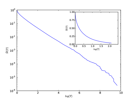
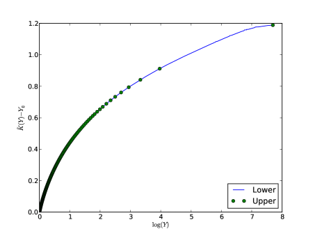
Figure 4 illustrates the details of the NLA applied to this computation. Panel (a) plots ${\tilde{M}}$ from equation (25). The run of ${\tilde{M}}$ with $Y$ rises rapidly near the posterior mode and drops rapidly to zero for small likelihood values. The inset in this figure shows ${\tilde{M}}$ in linear scale. The measure function ${\tilde{M}}$, and hence the integral ${\tilde{K}}$, is dominated by large values of $L$ as long as $M$ decreases sufficiently fast (see §3.1). Panel (b) plots the accumulating sum defining the quadrature of ${\tilde{Z}}$ in equations (9)–(12), beginning with the largest values of likelihood first. The contribution to ${\tilde{Z}}$ is dominated at the likelihood peak, corresponding to the steeply rising region of ${\tilde{M}}$ in Panel (a). In other words, the samples with small values of $L$ that degrade the HMA make a negligible contribution to the marginal likelihood computation as long as $h_{i}<h_{\ast}$. In addition, NLA provides upper and lower bounds, and thereby some warning when the estimate is poorly conditioned, e.g. owing to an inappropriate choice for $h_{\ast}$. The plot in Figure 4b will readily reveal such failures.

(a) $-0.2<{\bar{x}}<1.2$

(b) $0.2<{\bar{x}}<0.8$

(c) $0.4<{\bar{x}}<0.6$

(d) $0.46<{\bar{x}}<0.54$

Figure 5: Histogrammed distributions of ${\tilde{T}}$ for the NLA, VTA, HMA, and the Laplace approximation for 10,000 randomly resampled states of a converged posterior distribution of 200,000 states. The dashed line shows the true value computed by directly integrating $Z$ from eq. 2. Each panel is labeled by the range of the flat prior distribution for the position of the normal distribution.

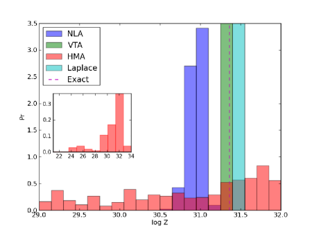
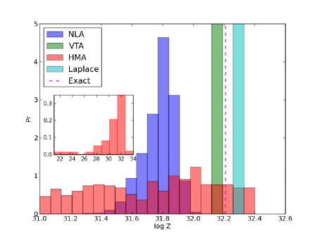
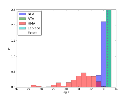
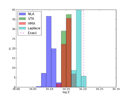
A more realistic error assessment can be obtained by subsampling the sequence $\{L_{k}\}$. The CPU time for these algorithms is sufficiently small that this procedure should be practical in general. Consider the following experiment: (1) the posterior is simulated by MCMC (as described above) to obtain a chain of 400,000 states; (2) the first half of the chain is discarded; (3) the second-half is randomly subsampled with replacement to obtain 128 samples of 10,000 states; (4) the marginal likelihood for each is computed using the NLA, VTA, the Laplace approximation and the HMA (approximately 2 CPU minute in total). For all but the HMA, increasing the number of states decreases the variance for each distribution; samples with 10,000 states best revealed the differences between the algorithms with a single scale.

Figure 5 illustrates the relative performance with different prior distributions. Figure 5a is the model described at the beginning of this section; the range of the prior distribution is much larger than the values sampled from the posterior distribution. The prior distributions for each successive panel have smaller ranges as indicated. The colors are composited with $\alpha=0.5$ (e.g. HMA over VTA is brown, HMA over NLA is purple, Laplace over HMA is blue-grey, Laplace over VTA is blue-green). In Panel (d), the range is within the range of values sampled by the posterior in Panel (a). The overall trends are as follows: 1) the HMA has unacceptably large variance unless the domain of the prior roughly coincides with the domain sampled by the MCMC algorithm; 2) the VTA and Laplace approximation have the smallest variances, followed by HMA; 3) the NLA is consistently biased below the analytic value; and 4) the VTA and Laplace approximation are closed to the expected analytic value. Indeed, the Laplace approximation is an ideal match to and should do well for this simple unimodal model. In the final panel, there are no outlier values of $L$ and the harmonic mean approximation is comparable to the others. These tests also demonstrate that the same outliers that wreck the HMA have much less affect on NLA and VTA. Further experimentation reveals that the results are very insensitive to the threshold value $h_{\ast}$. In fact, one needs an absurdly large value of $h_{\ast}$, $h_{\ast}>1$, to produce failure.

5.2 Non-nested Linear Regression Models

Here, we test these algorithms on the radiata pine compressive strength data analyzed by Han and Carlin (2001) and a number of previous authors. We use the data tabled by Han and Carlin from Williams (1959). These data describe the maximum compressive strength parallel to the grain $y_{i}$, the density $x_{i}$, and the resin-adjusted density $z_{i}$ for $N=42$ specimens. Carlin and Chib (1995) use these data to compare the two linear regression models:

$$M=1:y_{i} = \alpha+\beta(x_{i}-{\bar{x}})+\epsilon_{i},\,\,\,\quad\epsilon_{i}\sim{\cal N}(0,\sigma^{2}),\qquad i=1,\ldots,N$$

$$M=2:y_{i} = \gamma+\delta(z_{i}-{\bar{z}})+\epsilon_{i},\qquad\epsilon_{i}\sim{\cal N}(0,\tau^{2}),\qquad i=1,\ldots,N$$

with ${\cal M}=\{1,2\},\mathbb{\theta}_{1}=\{\alpha,\beta,\sigma^{2}\}^{T}$, and $\mathbb{\theta}_{2}=\{\gamma,\delta,\tau^{2}\}^{T}$. We follow Han and Carlin (2001) and Carlin and Chib (1995), adopting ${\cal N}\left(\{3000,185\}^{T},\mbox{Diag}\{10^{6},10^{4}\}\right)$ priors on $\{\alpha,\beta\}^{T}$ and $\{\gamma,\delta\}^{T}$, and $\mbox{IG}\left(3,[2*300^{2}]^{-1}\right)$ priors on $\sigma^{2}$ and $\tau^{2}$, where $\mbox{IG}(a,b)$ is the inverse gamma distribution with density function

$$f(v)=\frac{e^{-1/(bv)}}{\Gamma(a)b^{a}v^{a+1}}$$

where $v>0$ and $a,b>0$. Han and Carlin point out these priors are approximately centered on the least-squares solution but are otherwise rather vague. Using direct integration, Green and O’Hagan (1998) find a Bayes factor of about 4862 in favor of Model 2.

Table 1: Marginal likelihood for non-nested linear regression models

Model	$\log Z(M=1)$	$\log Z(M=2)$	$B_{21}$	$\Delta\%$
NLA	$-309.69\genfrac{}{}{0.0pt}{}{+0.07}{-0.10}$	$-301.20\genfrac{}{}{0.0pt}{}{+0.08}{-0.08}$	$4866\genfrac{}{}{0.0pt}{}{+965}{-707}$	0.1
VTA	$-308.30\genfrac{}{}{0.0pt}{}{+0.02}{-0.02}$	$-299.83\genfrac{}{}{0.0pt}{}{+0.02}{-0.02}$	$4741\genfrac{}{}{0.0pt}{}{+189}{-186}$	-2.5
HMA	$-379.99\genfrac{}{}{0.0pt}{}{+14.46}{-8.64}$	$-386.52\genfrac{}{}{0.0pt}{}{+23.16}{-7.74}$	$0\genfrac{}{}{0.0pt}{}{+10^{11}}{-0}$	-100.0
Laplace	$-306.66\genfrac{}{}{0.0pt}{}{+0.03}{-0.03}$	$-298.15\genfrac{}{}{0.0pt}{}{+0.03}{-0.04}$	$4974\genfrac{}{}{0.0pt}{}{+318}{-327}$	2.3

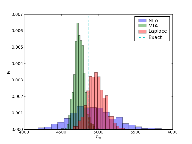
Table 1 describes the results of applying the algorithms from previous sections to a converged MCMC chain of 2.4 million states for both models using the parallel tempering scheme. The quoted value is the median and the bounds are the $p=0.025$ and $p=0.975$ quantiles computed from 1024 bootstrap samples of 100,000 states. I chose 100,000 state samples to achieve 95% confidence bounds of approximately 10% or smaller for both the NLA and VTA. The second and third columns of the table are the value of marginal likelihood for Models 1 and 2 for each of the four models listed in the first column. The quoted range is the 95% confidence bounds for each median value from the 1024 samples. The fourth column is the Bayes factor for Model 2 to Model 1 and the fifth column is the relative difference from the exact result. The NLA, VTA and Laplace approximation yield values within a few percent of the true value. The VTA presents the smallest variance, followed by Laplace and then NLA. The HMA samples are too broadly distributed to be of use. Figure 6 shows the distribution of $B_{21}$ for the samples; counter to the trend from §5.1, both the VTA and Laplace approximation are more biased than the NLA here.

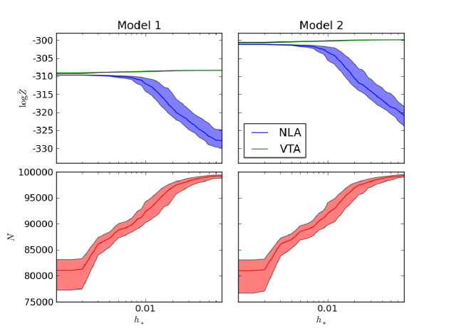
The value $h_{\ast}$ used to compute the NLA will vary with the problem and the sample size. Therefore, some analysis of ${\tilde{Z}}$ is required to choose an appropriate value. As an example, Figure 7 plots the median and 95% confidence region for the bootstrap sampled marginal likelihood computation as a function of $h_{\ast}$ for the regression problem. The value of the VTA for the same truncated sample is shown for reference only; truncation is not needed for the VTA. The values for ${\tilde{Z}}$ track each other closely for $0.001\leq h_{\ast}\leq 0.008$. For $h_{\ast}<0.001$, there are too few states for a reliable computation of ${\tilde{Z}}$. For $h_{\ast}>0.008$, the NLA values are sensitive to the low-likelihood tail, resulting in divergence with increasing $h_{\ast}$.

Figure 6: The histogrammed distribution of Bayes factors for the 1024 samples using the NLA, VTA and Laplace approximation. Although the variance for the NLA is larger than the VTA or Laplace approximation, its bias is small.

Figure 7: Comparison of the NLA and VTA as a function of $h_{\ast}$ for Models 1 and 2. The upper panel shows the run of ${\tilde{Z}}$ for increasing $h_{\ast}$; the lower panel shows the number of states out of 100000 that meet the $h_{\ast}$ threshold criterion. This increases to 100000 as $h_{\ast}$ increases; for a threshold $h_{\ast}=0.06$, approximately 100 states are rejected. The median (95% confidence region) is shown as a solid line (shaded band). The VTA 95% confidence region is nearly indistinguishable from the line width!

5.3 High-dimension parameter spaces

We adopt a ‘data-free’ likelihood function for parameter vector $\mathbf{\theta}$ with rank $k$:

$$L(\mathbf{\theta})=\left(2\pi\sigma^{2}\right)^{-k/2}e^{-\mathbf{\theta}^{2}/2\sigma^{2}}.$$

with $\sigma^{2}=\mbox{constant}$. Further, we assume that each parameter $\theta_{j}$ is normally distributed with a mean of 0 and a variance of 1. The resulting expression for the marginal likelihood may be directly integrated, yielding $P(\sigma^{2},k)=\left[2\pi(1+\sigma^{2})\right]^{k/2}$.

Table 2: Test of high-dimensional marginal likelihood

Model		NLA		VTA				Laplace
k	Exact	$\log{\tilde{Z}}$	$\Delta\%$	$\log{\tilde{Z}}_{0.1}$	$\log{\tilde{Z}}_{0.5}$	$\log{\tilde{Z}}_{0.9}$	$\Delta\%$	$\log{\tilde{Z}}$	$\Delta\%$
1	-1.468	$-1.45\genfrac{}{}{0.0pt}{}{+0.01}{-0.01}$	0.7	-1.45	$-1.45\genfrac{}{}{0.0pt}{}{+0.01}{-0.01}$	-1.45	0.7	$-1.60\genfrac{}{}{0.0pt}{}{+0.01}{-0.01}$	9.0
2	-2.936	$-2.94\genfrac{}{}{0.0pt}{}{+0.02}{-0.04}$	0.5	-2.92	$-2.92\genfrac{}{}{0.0pt}{}{+0.01}{-0.01}$	-2.92	0.5	$-3.20\genfrac{}{}{0.0pt}{}{+0.01}{-0.01}$	9.0
5	-7.341	$-7.31\genfrac{}{}{0.0pt}{}{+0.01}{-0.01}$	0.4	-6.90	$-7.35\genfrac{}{}{0.0pt}{}{+0.01}{-0.01}$	-7.48	0.1	$-7.99\genfrac{}{}{0.0pt}{}{+0.01}{-0.01}$	8.7
10	-14.68	$-14.47\genfrac{}{}{0.0pt}{}{+0.01}{-2.79}$	1.4	-14.56	$-14.44\genfrac{}{}{0.0pt}{}{+0.01}{-0.01}$	-14.34	1.6	$-16.06\genfrac{}{}{0.0pt}{}{+0.04}{-0.03}$	9.4
20	-29.36	$-29.23\genfrac{}{}{0.0pt}{}{+0.01}{-0.01}$	0.4	-29.38	$-29.14\genfrac{}{}{0.0pt}{}{+0.01}{-0.01}$	-28.91	0.7	$-32.38\genfrac{}{}{0.0pt}{}{+0.08}{-0.07}$	10
40	-58.73	$-59.51\genfrac{}{}{0.0pt}{}{+0.23}{-0.14}$	1.3	-59.69	$-59.01\genfrac{}{}{0.0pt}{}{+0.19}{-0.15}$	-58.97	0.9	$-56.59\genfrac{}{}{0.0pt}{}{+0.01}{-0.01}$	8.1

For each model of dimension $k$, we compute a Markov chain using the Differential Evolution algorithm (DE, Ter Braak,, 2006). This algorithm evolves an ensemble of chains with initial conditions sampled from the prior distribution. A proposal is computing by randomly selecting pairs of states from the ensemble and using a multiple of their difference; this automatically ‘tunes’ the proposal width. We have further augmented this algorithm by including a tempered simulation step (Neal,, 1996) after every 20 DE steps (see Weinberg,, 2010, for more details).

Each row describes of Table 2 describes the application of the NLA, VTA, and Laplace approximation to a model of dimension $k$. The MCMC simulations produce approximately 1.4 million converged states. Convergence is testing using the Gelman-Rubin statistic (op. cit.). Each converged chain is resampled with replacement to provide 1024 subsamples of $n$ states. The value $N\in[10000,400000]$ is chosen to achieve 95% confidence intervals approximately 1% of ${\tilde{Z}}$ or smaller. The 95% confidence intervals on ${\tilde{Z}}$ are indicated as sub- and super-scripts. Recall that the standard VTA determines volume spanned ${\bar{m}}$ samples and approximates the integral by multiplying the volume by the median value of the sample. To assess the variance inherent in this choice, I quote the results for two other p-quantiles, $p=0.1$ and $p=0.9$. Finally, for each algorithm, the table presents the relative error: $\Delta\%\equiv|{\log\tilde{Z}}-\log Z|/|\log Z|\times 100$.

Both the NLA and VTA results are very encouraging: the relative error is within a few percent for $1\leq k\leq 40$. For $k=40$, I computed ${\tilde{Z}}$ with samples sizes of 400,000 states. Both the NLA and VTA tend to slightly overestimate $Z$ for large $k$. The Laplace approximation results are disappointing for small $k$ and improve for large $k$, but still are less precise than either the NLA or VTA.

Figure 8: Two-dimensional illustration of the domain decomposition for the Gaussian likelihood example described in §5.3. The cells are colored according to posterior probability on a linear scale from 0 to $\sup\{P\}$.

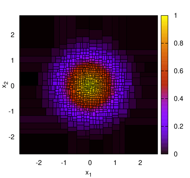
Figure 8 illustrates the kd-tree construction for a single $k=2$ sample. Each two-dimensional cell is colored by the median value of the posterior probability for the ${\bar{m}}=32$ points in each cell and scaled to the peak value of posterior probability $P$ for the entire sample. A careful by-eye examination of the cell shape reveals a preponderance of large axis-ratio rectangles; this is a well-known artifact of the kd-tree algorithm. For large values of $P$, the volume elements are small, and with a sufficiently large sample, the gradient in $P$ across the volume are small. For small values of $P$, the volume elements are large, the gradients are large, and the large-axis ratio rectangles distort the reconstructed shape of the true posterior. However, as described in §3.2, the values of $\pi(\boldsymbol{\theta})L({\bf D}|\boldsymbol{\theta})\Delta V=\mbox{constant}$ for an infinite sample, so a small number of distorted rectangles will not compromise the end result. Moreover, the values of $\pi(\boldsymbol{\theta})L({\bf D}|\boldsymbol{\theta})\Delta V$ at large volumes are smaller than those at small volume for these tests, and this further decreases the importance of the kd-tree cell-shape artifact.

5.4 Model selection

(a) $x\sim{\cal N}(0.5,0.03)$

(b) $x\sim\mbox{Cauchy}(0.5,\sqrt{0.03})$

Figure 9: A histogrammed distribution of the 1000 data points from ${\cal N}(0.5,0.03)$ Panel (a) and 100 data points from ${\cal C}(0.5,\sqrt{0.03})$ Panel (b) used in these examples compared with the “best fit” Normal and Cauchy distributions chosen from the peak of the posterior distribution.

Figure 10: Box and whisker plot for the distribution of the $\log{\tilde{Z}}$ but for a sample from the Cauchy distribution from Fig. 9. The box shows the quantiles and median, the whisker shows the (10%, 90%) intervals, followed by outlying points. The three distributions are (1) the HMA; (2) NLA for ${\tilde{K}}$ and VTA for ${\tilde{J}}$; and (3) VTA for both ${\tilde{J}}$ and ${\tilde{Z}}$.

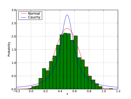
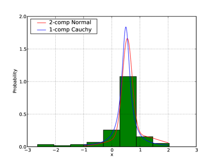
As an example of model selection, we first compute the marginal likelihood for the same data $x\sim{\cal N}(0.5,0.03)$ as in the first example of §5.1 but assuming a Cauchy-Lorentz distribution,

$${\cal C}(a,b):P(x|a,b)=\left[\pi b\left(1+\frac{(x-a)^{2}}{b^{2}}\right)\right]^{-1},$$

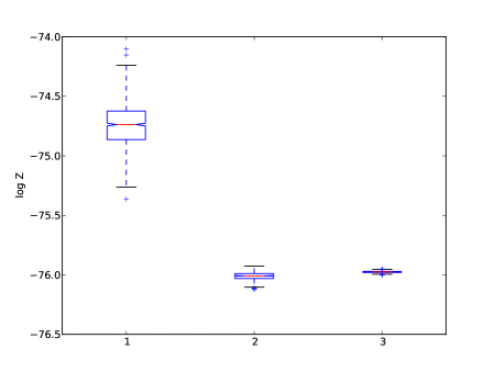
as the model with unknown location $a$ and scale $b$ parameters. For prior distributions, we take $a\sim{\cal U}(0,1)$ and $b\sim{\cal W}(0.025,1)$ where ${\cal W}(\lambda,k)$ is the Weibull distribution with scale parameter $\lambda$ and shape parameter $k$. NLA yields $\log{\tilde{Z}}=5.10^{+0.03}_{-0.03}$, VTA yields $\log{\tilde{Z}}=5.12^{+0.02}_{-0.01}$ and the HMA yields $\log{\tilde{Z}}=6.62^{+0.80}_{-119}$. The data and fits are shown in Figure 9a. There should be no surprise that the true model (with $\log Z=33.5$)is strongly preferred. Let us now repeat the experiment using 100 data points selected from the Cauchy-Lorentz distribution (${\tilde{Z}}_{1}$) and compare the marginal likelihood values for a Cauchy-Lorentz distribution and a mixture of two Normal distributions (${\tilde{Z}}_{2}$). NLA and VTA, respectively, yield $\log{\tilde{Z}}_{1}=-76.3^{+0.04}_{-0.04},-76.1^{+0.01}_{-0.01}$ and $\log{\tilde{Z}}_{2}=-136.9^{+0.2}_{-0.6},-134.4^{+1.1}_{-0.6}$. The HMA yields $\log{\tilde{Z}}_{1}=-75.9^{+0.01}_{-0.01}$ and $\log{\tilde{Z}}_{2}=-116.5^{+1.3}_{-0.9}$. Regardless of the algorithm performing the test, the Bayes factor reveals strong evidence in favor of the true model. Note from Figure 9b that both models are reasonable fits “by eye”. However, the Bayes factor overwhelmingly prefers the simpler (in this case, true) model. As expected, the distribution of ${\tilde{Z}}$ for the heavy-tailed Cauchy distribution is much better behaved (see Fig. 10). The results for NLA and VTA are consistent and the HMA is systematically larger, but non enough to misguide a decision.

6 Discussion and Summary

In summary, much of the general measure-theoretic underpinning of probability and statistics naturally leads naturally to the evaluation of expectation values. For example, the harmonic mean approximation (HMA, Newton and Raftery,, 1994) for the marginal likelihood has large variance and is slow to converge (e.g. Wolpert,, 2002). On the other hand, the use of analytic density functions for the likelihood and prior permits us to take advantage of less general but possibly more powerful computational techniques. In §§1–4 we diagnose the numerical origin of the insufficiencies of the HMA using Lebesgue integrals. There are two culprits: 1) the integral on the left-hand side of equation (3) may diverge if the measure function $M(Y=L^{-1})$ from equation (24) decreases too slowly; and 2) truncation error may dominate the quadrature of the left-hand side of equation (3) unless the sample is appropriately truncated. Using numerical quadrature for the marginal likelihood integral (eqns. 2 and 24) leads to improved algorithms: the Numerical Lebesgue Algorithm (NLA) and the Volume Tessellation Algorithm (VTA). Our proposed algorithms are a bit more difficult to implement and have higher computational complexity than the simple HMA, but the overall CPU time is rather modest compared to the computational investment required to produce the MCMC-sampled posterior distribution itself. For a sample of size $N$, the sorting required by NLA and VTA has computational complexity of ${\cal O}(N\log N)$ and ${\cal O}(N\log^{2}N)$, respectively, rather than ${\cal O}(N)$ for the harmonic mean. Nonetheless, the computational time is a fraction of second to minutes for typical values of $10^{5}<N<10^{8}$ (see §4).

The geometric picture behind NLA is exactly that for Lebesgue integration. Consider integrating a function over a two-dimensional domain. In standard Riemann quadrature, one chops the domain into rectangles and adds up their area. The sum can be refined by subdividing the rectangles; in the limit of infinitesimal area, the resulting sum is the desired integral. In the Lebesgue approach, one draws horizontal slices through the surface and adds up the area of the horizontal rectangles formed from the width of the slice and the vertical distance between slices. The sum can be refined by making the slices thinner when needed; in the limit of slices of infinitesimal height, the resulting sum is the desired integral. In the Riemann case, we multiply the box area in the domain, $dA$, by the function height, $f$. In the Lebesgue, we multiply the slice height in the range, $df$, by the domain area, $A$ (see Fig. 1). Both algorithms easily generalize to higher dimension. For the Lebesgue integral, the slices become level sets on the hypersurface implied by the integrand. Therefore the Lebesgue approach always looks one-dimensional in the level-set value; the dimensionality $k$ is ‘hidden’ in the area of domain (hypervolume $A$ for $k>3$) computed by the measure function $M(Y)$. The level-set value for the NLA is $Y=1/L({\bf D}|\boldsymbol{\theta})$. Once determined, NLA applies the trapezoidal rule to the sum over slices and compute the upper and lower rectangle sums as bounds. Clearly, the error control on this algorithm might be improved by using more of the information about the run of $A$ with $f$.

Having realized that the practical failure of the harmonic mean approximation is a consequence of the sparsely sampled parameter-space domain, NLA addresses the problem by determining a well-sampled subset $\Omega_{s}\subset\Omega$ from the MCMC sample, ex post facto. Restricted to this subset, $\Omega_{s}$, the value of the integral $J$ on the right-hand side of equation (3) is less than unity. We determine $\Omega_{s}$ by a binary space partitioning (BSP) tree and compute $J$ from this partition. A BSP tree recursively partitions a the k-dimensional parameter space into convex subspaces. The VTA is implemented with a kd-tree (Cormen et al.,, 2001) for simplicity. In addition, one may use VTA by itself to compute equation (2) directly.

Judged by bias and variance, the test examples do not suggest a strong preference for either the NLA or the VTA. However, both are clearly better than the HMA or the Laplace approximation. Conversely, because these algorithms exploit the additional structure implied by smooth, well-behaved likelihood and prior distribution functions, the algorithms developed here will be inaccurately and possibly fail miserably for wild density functions. The NLA and the VTA are not completely independent since the NLA uses the tessellation from the VTA to estimate the integral $J$. However, the value of the integral $K$ tends to dominate $Z$, that is $|\log K|\gg|\log J|$, and the contributions are easily checked. Based on current results, I tentatively recommend relying preferentially on VTA for the following reasons: 1) there is no intrinsic divergence; 2) it appears to do as well as VTA even in a high-dimensional space; and 3) there is no truncation threshold $h_{\ast}$.

Figure 8 illustrates the potential for volume artifacts that could lead to both bias and variance. This error source affects both the VTA and NLA (through the computation of ${\tilde{J}}$) but the affect on the NLA may be larger (§5.1). Additional real-world testing, especially on high-dimensional multimodal posteriors, will provide more insight. In test problems described in this paper, I explored the effects of varying the threshold $h_{\ast}$ and the kd-tree bucket size ${\bar{m}}$. These parameters interact the sample distribution, and therefore, are likely to vary for each problem. I also recommend implementing both the NLA, VTA, HTM, Laplace approximation and comparing the four for each problem. We are currently testing these algorithms for astronomical inference problems too complex for a simple example; the results will be reported in future papers. An implementation of these algorithms will be provided in the next release of the UMass Bayesian Inference Engine (BIE, Weinberg,, 2010).

There are several natural algorithmic extensions and improvements not explored here. §2 describes a smoothed approximation to the computation of $M(Y)$ (eqns. 13–16) rather than the step function used in §4. The direct integration of equation (2) currently ignores the location of field values in each cell volume. At the expense of CPU time, the accuracy might be improved by fitting the sampled points with low-order multinomials and using the fits to derive a cubature algorithm for each cell. In addition, a more sophisticated tree structure may decrease the potential for bias by providing a tessellation with “rounder” cells.

In conclusion, the marginal likelihood

$$Z=\int d\boldsymbol{\theta}\pi(\boldsymbol{\theta}|{\cal M})L({\bf D}|\boldsymbol{\theta},{\cal M})$$

may be reliably computed from a Monte Carlo posterior sample though careful attention to the numerics. We have demonstrated that the error in the HMA is due to samples with very low likelihood values but significant prior probability. It follows that their posterior probability also very low, and these states tend to be outliers. On the other hand, the converged posterior sample is a good representation of the posterior probability density by construction. The proposed algorithms define the subdomain $\Omega_{s}\subset\Omega$ dominated by and well-sampled by the posterior distribution and perform the integrals in equation (3) over $\Omega_{s}$ rather than $\Omega$. Although more testing is needed, these new algorithms promise more reliable estimates for $Z$ from an MCMC simulated posterior distribution with more general models than previous algorithms can deliver.

References

- Capinski and Kopp, (2007) Capinski, M. and Kopp, P. E. (2007). Measure, Integral and Probability. Springer, 2nd edition.
- Chib and Jeliazkov, (2001) Chib, S. and Jeliazkov, I. (2001). Marginal likelihood from the Metropolis-Hastings output. Journal of the American Statistical Association, 96(453):270–281.
- Cormen et al., (2001) Cormen, T. H., Leiserson, C. E., Rivest, R. L., and Stein, C. (2001). Introduction to Algorithms. The MIT Press, 2nd edition.
- DiCicio et al., (1997) DiCicio, T., Kass, R., Raftery, A., and Wasserman, L. (1997). Computing Bayes factors by combining simulation and asymptotic approximations. American Statistical Association, 92:903–915.
- Edelsbrunner and Shah, (1966) Edelsbrunner, H. and Shah, N. (1966). Incremental topological flipping works for regular triangulations. Algorithmica, 15(3):223–241.
- Feroz and Hobson, (2008) Feroz, F. and Hobson, M. P. (2008). Multimodal nested sampling: an efficient and robust alternative to Markov chain Monte Carlo methods for astronomical data analyses. Mon. Not. R. Astron. Soc., 384(2):449–463.
- Gelman et al., (2003) Gelman, A., Carlin, J. B., Stern, H. S., and Rubin, D. B. (2003). Bayesian Data Analysis. Texts in Statistical Science. CRC Press, Boca Raton, FL, 2nd edition.
- Gelman and Rubin, (1992) Gelman, A. and Rubin, D. B. (1992). Inference from iterative simulation using multiple sequences. Statistical Science, 7:457–472.
- Geyer, (1991) Geyer, C. (1991). Markov chain Monte Carlo maximum likelihood. In Computing Science and Statistics, Proceedings of the 23rd Symposium on the Interface, page 156. American Statistical Association.
- Giakoumatos et al., (1999) Giakoumatos, S. G., Vrontos, I. D., Dellaportas, P., and Politis, D. N. (1999). An MCMC convergence diagnostic using subsampling. Journal of Computational and Graphical Statistics, i:431–451.
- Green, (1995) Green, P. J. (1995). Reversible jump Markov chain Monte Carlo computation and Bayesian model determination. Biometrika, 82:711–32.
- Kass and Raftery, (1995) Kass, R. E. and Raftery, A. E. (1995). Bayes Factors. Journal of the American Statistical Association, 90(430):773–795.
- Lavine and Schervish, (1999) Lavine, M. and Schervish, M. (1999). Bayes Factors: What they are and what they are not. American Statistician, 53:119–122.
- Meng and Wong, (1996) Meng, X.-L. and Wong, W. H. (1996). Simulating ratios of normalizing constants via a simple identity: A theoretical exploration. Statistica Sinica, 6:831–860.
- Mukherjee et al., (2006) Mukherjee, P., Parkinson, D., and Liddle, A. R. (2006). A nested sampling algorithm for cosmological model selection. ApJ, 638(2):51–54.
- Neal, (1996) Neal, R. M. (1996). Sampling from multimodal distributions using tempered transitions. Statistics and Computing, 6:353–366.
- Newton and Raftery, (1994) Newton, M. A. and Raftery, A. E. (1994). Approximate Bayesian inference by the weighted likelihood bootstrap. J. Roy. Statist. Soc. B, 56:3–48.
- Raftery et al., (2007) Raftery, A. E., Newton, M. A., Satagopan, J. M., and Krivitsky, P. N. (2007). Estimating the integrated likelihood via posterior simulation using the harmonic mean identity. Bayesian Statistics, 8(1-45).
- Skilling, (2006) Skilling, J. (2006). Nested sampling for general Bayesian computation. Bayesian Analysis, 1(4):833–860.
- Temple, (1971) Temple, G. (1971). The Structure of Lebesgue Integration Theory. Oxford University Press.
- Ter Braak, (2006) Ter Braak, C. J. F. (2006). A Markov chain Monte Carlo version of the genetic algorithm Differential Evolution: easy Bayesian computing for real parameter spaces. Stat. Comput., 16:239–249.
- Trotta, (2007) Trotta, R. (2007). Applications of Bayesian model selection to cosmological parameters. Mon. Not. R. Astron. Soc., 378:72–82.
- Trotta, (2008) Trotta, R. (2008). Bayes in the sky: Bayesian inference and model selection in cosmology. Contemporary Physics, 49(2):71–104.
- Weinberg, (2010) Weinberg, M. D. (2010). The UMass Bayesian Inference Engine. Mon. Not. R. Astron. Soc. in preparation, see http://www.astro.umass.edu/BIE.
- Wolpert, (2002) Wolpert, R. L. (2002). Stable limit laws for marginal probabilities from MCMC streams: Acceleration of convergence. Discussion Paper 2002-22, Duke University ISDS.