An entropy-based approach to automatic image segmentation of satellite images

Abstract

An entropy-based image segmentation approach is introduced and applied to color images obtained from Google Earth. Segmentation refers to the process of partitioning a digital image in order to locate different objects and regions of interest. The application to satellite images paves the way to automated monitoring of ecological catastrophes, urban growth, agricultural activity, maritime pollution, climate changing and general surveillance. Regions representing aquatic, rural and urban areas are identified and the accuracy of the proposed segmentation methodology is evaluated. The comparison with gray level images revealed that the color information is fundamental to obtain an accurate segmentation.

I Introduction

Medical, biological and astronomical experiments, as well as satellite prospection, have generated terabytes of image data, making automatic analysis a fundamental resource for knowledge discovery. Image analysis is based on the extraction of meaningful information and can involve many steps, such as pre-processing (e.g. noise removing), segmentation and characterization of the identified objects da2001shape . Particularly, the identification of the types of objects — a task called segmentation — constitutes an essential issue in pattern recognition da2001shape due to its practical importance, such as in the treatment of images obtained from satellite prospection. In fact, image segmentation can be understood as the process of assigning a label to every pixel in an image, such that pixels with the same label represent the same object, or its parts

In the current work, we propose an entropy-based segmentation of images. The methodology is evaluated with respect to satellite images obtained from Google Earth, in order to identify aquatic, urban and rural regions. The importance of using Google Earth images can be observed in a growing number of investigations, such as the analysis of magnetic alignment of cattle and deer during grazing and resting begall105mag or mapping of disaster zones for identifying priorities, planning logistics and definition of access routes for relief operations nourbakhsh2006mdz . In fact, satellite images are critically important for the monitoring of ecological catastrophes, urban growth, agricultural activity, maritime pollution, climate changing as well as general surveillance. Moreover, the segmentation of Google Earth images is particularly important for automatic mapping of urban and rural areas while monitoring dynamical human activities, such as city growth that can affect regions of environmental preservation. Another application involves monitoring of rural activities, which can also lead to different textures, such as those observed in cultivation of sugarcane or wheat. The identification of aquatic areas allows the monitoring of pollution, which can be potentially inferred from changes in the water texture, as well as the formation of deserts or marshes, i.e. it provides an indication about possible climate changes. In addition, analysis of satellite images can help in monitoring of deforestation and in finding focuses of fires in forests.

Images are composed by a set of pixels whose values encode different colors or gray levels. Image segmentation methods have been used to find regions of interest (e.g. objects) in images. The importance of image segmentation can be illustrated in diverse practical applications, such as in medical imaging (e.g. diagnosis noble2006uis ), satellite images masson1993sem , face recognition zhao2003face , traffic control system cucchiara2000image and machine vision haralick1992computer . Different algorithms have been proposed for image segmentation such as those founded on image thresholding (e.g. by means of histograms of gray levels navon2005cis ); clustering methods (e.g neural networks kuntimad1999pis ); region growing methods (e.g. haralick1985ist ); graph partitioning methods (e.g. shi2000nca ); multi-scale segmentation (e.g. kuijper2003ssh ), and semi-automated segmentation (e.g. mortensen1998isi ). Methods related to physics concepts have also been more and more applied for image segmentation, such as those based on Markov random fields celeux2003pum and entropy portesdealbuquerque2004itu . The segmentation approach proposed in the current work is based on the concept of entropy.

In next sections, the concepts of information entropy, dimensionality reduction and supervised classification are presented. Afterwards, the proposed image segmentation methodology is applied to images of the Google Earth and the classification results are evaluated. The influence of the parameters involved in the segmentation is discussed. Venues for future research and conclusions are identified.

II Methodology

In information theory, the concept of entropy is used to quantify the amount of information necessary to describe the macrostate state of a system cover1991eit . Therefore, the entropy is related to the concept of complexity bar2003dynamics . Then, if a system presents a high value of entropy, it means that much information is neccessary to describe its states. Depending of the specific application, the entropy can be defined in different ways. For instance, while in quantum mechanics, the entropy is related to the von Neumann entropy vonneumann1932mgq ; in complexity theory, it is associated to the Kolmogorov entropy li1997ikc . Here we take the concept of entropy in the sense of information theory (Shannon entropy), where entropy is used to quantify the minimum descriptive complexity of a random variable cover1991eit . The Shannon entropy of a discrete random distribution $p(x)$ is defined as

$$H(p)=-\sum_{x}p(x)\log p(x),$$ (1)

where the logarithm is taken on the base 2.

In image analysis, $p(x)$ can refer to the distribution of gray levels or to the intensity of different color components of an image. The histograms $p(x)$ of a color image are obtained by counting the number of pixels with a given color intensity (red (R), green (G) or blue (B)), which can vary from 0 to 255. In this way, this procedure generates a set of three different histograms $\{h_{c}(x)\}$, where $c=\{R,G,B\}$. Due to its particular nature, as discussed above, the entropy can provide a good level of information to describe a given image. In this case, if all pixels in an image have the same gray level or the same intensity of color components, this image will present the minimal entropy value. On the other hand, when each pixel of an image presents a specific gray level or a color intensity, it this image will exhibit maximum entropy. Thus, since the pixel intensities are related to texture, because different textures tend to result in different distribution of gray level or color intensity, the Shannon entropy can be used for texture characterization da2001shape . Our texture approach is based on this assumption about texture analysis. The application to satellite images is justified because these images are formed by objects presenting different textures. In fact, different regions in these images, such as aquatic and urban areas, tend to present specific textures which are possibly characterized by different entropy values. For instance, while urban areas tend to exhibit high color variations (higher entropy), aquatic regions tend to be more homogeneous (lower entropy).

Our proposed methodology for segmentation of satellite images is performed as follows. Images are divided into square windows with a fixed size $L$, the entropy is calculated for each window, and then a classification methodology is applied for the identification of the category of the respective windows (e.g. aquatic, rural, urban, etc.). The classification approach can be supervised or non-supervised. Supervised classification needs a training set composed by windows whose classes are previously known (prototypes), such as rural and urban areas. Here, we focus on a segmentation methodology based on supervised classification. Initially, the training is done by selecting samples (windows) of the three types of regions (i.e. aquatic, rural and urban areas). Observe that each of these sample windows should be selected in order to present pixels of only one class. Next, the entropy is calculated for each color component (R,G and B) of these windows. Therefore, these windows are represented in a three-dimensional space defined by the entropy of the colors components, i.e. each window is represented by a vector with three elements. Then, due to the high correlation between the entropy of color components, these windows are projected into a one dimensional space by considering principal component analysis jolliffe2002principal . Note that the projection into one dimension by principal component analysis allows to optimally remove the redundancy present in the data. Finally, the classification of the training set is performed.

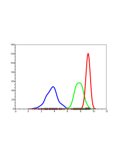
The classification is done by maximum likelihood decision theory, which considers the density functions estimated for each class duda2001pattern . This estimation is obtained by the Parzen windows approach duda2001pattern , which adds a normalized Gaussian function at each observation point, so that the interpolated densities correspond to the sum of these functions, performed separately for each class (see Figure 2). These densities are used in the maximum likelihood approach. If the probability density is known, it can be showed that this classification approach is optimal in the sense of minimizing misclassification duda2001pattern . The second step in the supervised classification is performed by classifying unknown windows. In this way, it is possible to evaluate the accuracy of the classifier by comparing the resulting classification and the original regions. In fact, the evaluation of the precision of the classification approach is given by the confusion matrix $C$, whose elements $c_{ij}$ provide the number of windows of class $j$ which were classified as being of class $i$ da2001shape . The percentage of correct classification is obtained by the sum of the confusion matrix diagonal divided by the total sum of the matrix.

III Results and discussion

Figure 1: The scatterplot of the entropies of the windows with sizes (a) $16\times 16$, (b) $30\times 30$ and (c) $46\times 46$. Each point corresponds to a window, represented by the three coordinates associated to the entropies of each of the three color components (R, G and B). Windows corresponding to water, rural and urban regions are represented by blue triangle, green circles and red squares, respectively. These windows correspond to the training step of the supervised classification.

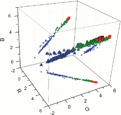
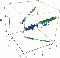
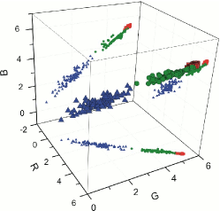
In order to segment images of the Google Earth, we took into account square windows of dimensions $16\times 16$, $30\times 30$ and $46\times 46$ pixels. We obtained $100$ windows of each class and calculated the entropy distribution for each color component from the respective histograms. Figure 1 presents the windows in the space defined by the entropy of the three color components. Note that the urban and rural regions present a small intersecting region, because urban areas can exhibit trees and parks, which present textures similar to those present in rural areas. Since these windows are approximately organized as a straight line in the three-dimensional scatterplot, which indicates a strong correlation between the entropies of color components, we projected the entropies into a one-dimensional space by applying principal component analysis jolliffe2002principal . The variances of this type of projection corroborate the one-dimensional organization of the points, i.e. the first eigenvalue divided by all eigenvalues is equal to $\lambda_{1}/\sum_{i=1}^{3}\lambda_{i}=0.99$ for all windows sizes. In other words, the projected data accounts for $99\%$ of the variance of the original observations. To obtain the density function, we considered the Parzen windows approach, as described before.

Figure 2 illustrates the obtained probability densities. After estimation, we performed the classification by maximum likelihood decision theory, which uses the Bayes rule, associating each image window to the class that results in the largest probability duda2001pattern . Figure 2 shows that the larger the windows sizes, the larger are the intersections between the curves. In addition, urban and rural areas present the largest intersecting region, because some urban areas are composed by trees, woods and parks.

Figure 2: Probability densities estimated for windows of size (a) 16, (b) 30 and (b) 46. The projections were obtained from the scatterplots of Figure 1. The windows correspond to water, rural and urban regions are represented by blue triangle, green circles and red squares, respectively.

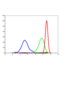
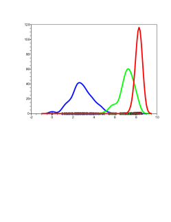
In order to evaluate the precision of our methodology, we segmented $10$ images manually and compared these original segmentations with those obtained from our classification methodology. The regions were extracted from cities from different worldwide zones, such as Berlin, Hong Kong, New York, Buenos Aires, Washington, Warsaw, Madrid, and Baghdad. The images were obtained at the same altitude ($2,000$ meters), in order to incorporate the same level of details in each sample. Tables 1, 2 and 3 present the confusion matrices. Notice that these matrices were calculated by taking into account each pixel on the image, and not each window, because some windows are composed by more than one class of pixels. The adoption of small windows, i.e. $16\times 16$ and $30\times 30$, accounted to a more accurate classification than the larger one ($46\times 46$). This happens because small windows tend to include regions with more homogeneous classes, while more heterogeneous regions tend to be included within larger windows. Nevertheless, the precision obtained with smaller windows is achieved at the expense of higher computational cost, due to the larger number of required windows to be processed. Comparing the percentage of correct classification given in each confusion matrix, we conclude that the highest errors occurs for the aquatic and rural regions with respect to windows of size $46\times 46$, where $24\%$ of aquatic regions were classified as rural regions, and $24\%$ of rural regions were classified as urban. In the former case, the error has been verified to be a consequence of texture similarities between some rivers that present a high level of green algae and some types of plantations, which are predominantly based on green vegetables. In the latter case, urban and rural regions tend to share similar green areas. The highest score ($90\%$) was obtained by aquatic regions taking into account windows of size $16\times 16$. The accuracy of our classification methodology can be summarized in terms of the sum of the confusion matrix diagonal divided by the total sum of the matrix. We indicate this ratio by $\alpha_{L}$, where $L$ is the window size. The obtained values are equal to $\alpha_{46}=0.79\pm 0.07$ for windows of size $46\times 46$, $\alpha_{30}=0.85\pm 0.03$ for windows of size $30\times 30$ and $\alpha_{16}=0.85\pm 0.04$ for windows of size $16\times 16$. Therefore, the smallest windows provide the most precise segmentation.

Table 1: Confusion matrix for $10$ segmented images taking into account windows of size $16\times 16$. The overall accuracy in this case is equal to $\alpha_{16}=0.85\pm 0.04$.

Confusion	urban	rural	aquatic
urban	0.83$\pm 0.07$	0.17$\pm 0.07$	0.00$\pm 0.00$
rural	0.17$\pm 0.09$	0.82$\pm 0.09$	0.01$\pm 0.03$
aquatic	0.00$\pm 0.00$	0.10$\pm 0.06$	0.90$\pm 0.06$

Table 2: Confusion matrix for $10$ segmented images taking into account windows of size $30\times 30$. The overall accuracy in this case is equal to $\alpha_{30}=0.85\pm 0.03$.

Confusion	urban	rural	aquatic
urban	0.87$\pm 0.05$	0.13$\pm 0.05$	0.00$\pm 0.00$
rural	0.13$\pm 0.07$	0.86$\pm 0.06$	0.01$\pm 0.02$
aquatic	0.01$\pm 0.01$	0.17$\pm 0.10$	0.82$\pm 0.11$

Table 3: Confusion matrix for 10 segmented images taking into account windows of size $46\times 46$. The overall accuracy in this case is equal to $\alpha_{46}=0.79\pm 0.07$

Confusion	urban	rural	aquatic
urban	0.88$\pm 0.06$	0.11$\pm 0.06$	0.01$\pm 0.01$
rural	0.24$\pm 0.12$	0.75$\pm 0.11$	0.01$\pm 0.02$
aquatic	0.02$\pm 0.02$	0.24$\pm 0.16$	0.74$\pm 0.17$

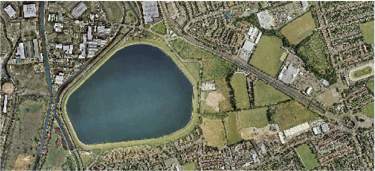
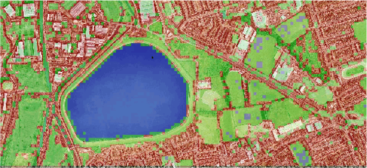
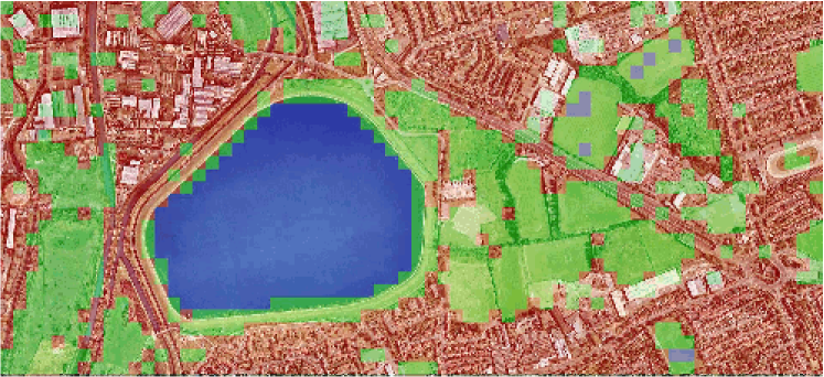
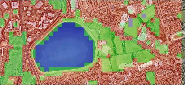
An additional analysis of our classification methodology was performed with respect to the segmentations of a region of London (obtained at $2,000$ meters of altitude), as presented in Figures 3 for windows of dimensions $16\times 16$, $30\times 30$ and $46\times 46$. The smallest windows ($16\times 16$) provide the most accurate segmentation, mainly with respect to the boundaries of the rural, aquatic and urban regions. Nevertheless, at the same time, due to the small size of the windows, some parts of urban areas are classified as rural as a consequence of the presence of trees, woods and parks. In fact, due to the level of details of the image, some windows corresponding to urban areas can be completely formed by trees – windows composed by green areas typically correspond to rural regions. As we increase the size of the windows, the observed misclassification is reduced, but the boundaries of each region tend to become less defined. This effect can be observed along the boundary of the aquatic area. Indeed, the effect of the green regions in urban area segmentation can be verified by the comparison of the confusion matrices obtained for windows of size $16\times 16$ and $30\times 30$, Tables 1 and 2. These tables show that the former case results in a larger error in classification of urban regions, mainly due to the classification of urban trees as rural areas. These misclassifications implied in similar scores for windows of dimensions $16\times 16$ and $30\times 30$. Indeed, the more accurate segmentation of the boundary of the regions are compensated by the wrong classification of urban green areas. Despite the wrong segmentation of these areas, we can observe that more accurate classifications can be obtained for smaller windows. Larger windows tend to provide worse classification because many of these windows in the segmented image can be compose by more than one class of regions. In fact, most of the misclassifications occur with respect to these windows.

Figure 3: A region of London and its respective segmentation by taking into account windows of size (a) 16, (b) 30 and (c) 46.

In order to compare our obtained results with a more traditional approach, we took into account gray level versions of the considered images. We adopted the same methodology used for color images to obtain the segmentation, but each image was now represented by a vector with only one element (the entropy of gray level histograms). Note that for color images, three color components were used and the images were represented by a vector composed by three elements. Tables 4, 5 and 6 show the obtained confusion matrices for windows of dimensions $16\times 16$, $30\times 30$ and $46\times 46$, respectively. In these cases, the sum of the confusion matrix diagonal divided by the total sum of the matrix are equal to $\alpha_{16}=0.74\pm 0.10$, $\alpha_{30}=0.75\pm 10$ and $\alpha_{46}=0.73\pm 0.10$. It is nteresting to observe that the different windows sizes resulted in similar classification performances. Comparing with the results obtained for color images, the gray level resulted in worse classification. Therefore, the spectral color information is critically important for achieving accurate segmentation.

Table 4: Confusion matrix for $10$ segmented gray images taking into account windows of size $16\times 16$. The overall accuracy in this case is equal to $\alpha_{16}=0.74\pm 0.10$

Confusion	urban	rural	aquatic
urban	0.74$\pm 0.20$	0.26$\pm 0.20$	0.00$\pm 0.00$
rural	0.11$\pm 0.09$	0.89$\pm 0.09$	0.00$\pm 0.01$
aquatic	0.02$\pm 0.05$	0.38$\pm 0.28$	0.60$\pm 0.27$

Table 5: Confusion matrix for $10$ segmented gray images taking into account windows of size $30\times 30$. The overall accuracy in this case is equal to $\alpha_{30}=0.75\pm 0.10$

Confusion	urban	rural	aquatic
urban	0.74$\pm 0.22$	0.26$\pm 0.22$	0.00$\pm 0.00$
rural	0.09$\pm 0.09$	0.91$\pm 0.08$	0.01$\pm 0.01$
aquatic	0.01$\pm 0.02$	0.39$\pm 0.26$	0.59$\pm 0.26$

Table 6: Confusion matrix for 10 segmented gray images taking into account windows of size $46\times 46$. The overall accuracy in this case is equal to $\alpha_{46}=0.73\pm 0.10$

Confusion	urban	rural	aquatic
urban	0.75$\pm 0.22$	0.24$\pm 0.22$	0.01$\pm 0.01$
rural	0.10$\pm 0.10$	0.89$\pm 0.10$	0.01$\pm 0.01$
aquatic	0.02$\pm 0.04$	0.39$\pm 0.26$	0.59$\pm 0.25$

IV Conclusion

Despite its simplicity, the described methodology revealed to be particularly accurate and effective for the classification of geographical regions. Indeed, we have shown that the entropy of the color distribution in images of geographical regions conveys enough information about the respective type of terrain so as to ensure a particularly high number of correct classifications, making of the proposed methodology an operational approach to be used in several related problems. Although the best classification rate obtained was equal to $0.90$, more accurate classification could be obtained by taking into account windows of smaller sizes than those we used here. Other statistical measurements, such as statistical moments, can also be used to complement the characterization of the texture of geographical regions. The extension of the current methodology to other types of regions, such as different types of forest or agricultural activities, is straightforward. In addition, the classification methodology can be improved by considering smaller windows combined with image pre-processing techniques, such as color equalization or noise removal. Other types of classifiers, such as support vector machine or neural networks bishop2006pattern can also be used.

V Acknowledgments

Luciano da F. Costa is grateful to FAPESP (proc. 05/00587-5), CNPq (proc. 301303/06-1) for financial support. Francisco A. Rodrigues acknowledges FAPESP sponsorship (proc. 07/50633-9). Odemir M. Bruno acknowledges sup port from CNPq (306628/2007-4 and 484474/2007-3).

References

- [1] L. da F. Costa and R.M. Cesar. Shape analysis and classification: theory and practice. CRC, 2001.
- [2] S. Begall, J. Červenỳ, J. Neef, O. Vojtěch, and H. Burda. Magnetic alignment in grazing and resting cattle and deer. Proceedings of the National Academy of Sciences, 105(36):13451.
- [3] I. Nourbakhsh, R. Sargent, A. Wright, K. Cramer, B. McClendon, and M. Jones. Mapping disaster zones. Nature, 439(7078):787–788, 2006.
- [4] J.A. Noble and D. Boukerroui. Ultrasound image segmentation: A survey. IEEE Transactions on medical imaging, 25(8):987–1010, 2006.
- [5] P. Masson and W. Pieczynski. SEM algorithm and unsupervised statistical segmentation ofsatellite images. IEEE Transactions on Geoscience and Remote Sensing, 31(3):618–633, 1993.
- [6] W. Zhao, R. Chellappa, PJ Phillips, and A. Rosenfeld. Face recognition: A literature survey. Acm Computing Surveys (CSUR), 35(4):399–458, 2003.
- [7] R. Cucchiara, M. Piccardi, and P. Mello. Image analysis and rule-based reasoning for a traffic monitoring system. IEEE Transactions on Intelligent Transportation Systems, 1(2):119–130, 2000.
- [8] R.M. Haralick and L.G. Shapiro. Computer and robot vision. Addison-Wesley Longman Publishing Co., Inc. Boston, MA, USA, 1992.
- [9] E. Navon, O. Miller, and A. Averbuch. Color image segmentation based on adaptive local thresholds. Image and vision computing, 23(1):69–85, 2005.
- [10] G. Kuntimad, HS Ranganath, R. Div, B.N. American, and AL Huntsville. Perfect image segmentation using pulse coupled neural networks. IEEE Transactions on Neural Networks, 10(3):591–598, 1999.
- [11] R. M. Haralick and L. G. Shapiro. Image segmentation techniques. Computer vision, graphics, and image processing, 29(1):100–132, 1985.
- [12] J. Shi and J. Malik. Normalized cuts and image segmentation. IEEE Transactions on pattern analysis and machine intelligence, 22(8):888–905, 2000.
- [13] A. Kuijper, L.M.J. Florack, and M.A. Viergever. Scale space hierarchy. Journal of Mathematical Imaging and Vision, 18(2):169–189, 2003.
- [14] E.N. Mortensen and W.A. Barrett. Interactive segmentation with intelligent scissors. Graphical Models and Image Processing, 60(5):349–384, 1998.
- [15] G. Celeux, F. Forbes, and N. Peyrard. EM procedures using mean field-like approximations for Markov model-based image segmentation. Pattern recognition, 36(1):131–144, 2003.
- [16] M. Portes de Albuquerque, IA Esquef, AR Gesualdi Mello, and M. Portes de Albuquerque. Image thresholding using Tsallis entropy. Pattern recognition letters, 25(9):1059–1065, 2004.
- [17] T.M. Cover, J.A. Thomas, J. Wiley, and W. InterScience. Elements of information theory. Wiley New York, 1991.
- [18] Y. Bar-Yam. Dynamics of complex systems. Westview Press, 2003.
- [19] J. von Neumann. Mathematische Grundlagen der Quantenmechanik (Mathematical Foundations of Quantum Mechanics). Springer, Berlin, 1955.
- [20] M. Li and P. Vitányi. An Introduction to Kolmogorov Complexity and Its Applications. Springer, 1997.
- [21] IT Jolliffe. Principal component analysis. Springer verlag, 2002.
- [22] R.O. Duda, P.E. Hart, and D.G. Stork. Pattern classification. Wiley New York, 2001.
- [23] C.M. Bishop et al. Pattern recognition and machine learning. Springer New York:, 2006.