Spatial and temporal dynamical heterogeneities approaching the binary colloidal glass transition

Takayuki Narumi,^a Scott V. Franklin,^b Kenneth W. Desmond,^c Michio Tokuyama,^d and Eric R. Weeks^∗c

We study concentrated binary colloidal suspensions, a model system which has a glass transition as the volume fraction $\phi$ of particles is increased. We use confocal microscopy to directly observe particle motion within dense samples with $\phi$ ranging from 0.4 to 0.7. Our binary mixtures have a particle diameter ratio $d_{S}/d_{L}=1/1.3$ and particle number ratio $N_{S}/N_{L}=1.56$, which are chosen to inhibit crystallization and enable long-time observations. Near the glass transition we find that particle dynamics are heterogeneous in both space and time. The most mobile particles occur in spatially localized groups. The length scales characterizing these mobile regions grow slightly as the glass transition is approached, with the largest length scales seen being $\sim 4$ small particle diameters. We also study temporal fluctuations using the dynamic susceptibility $\chi_{4}$, and find that the fluctuations grow as the glass transition is approached. Analysis of both spatial and temporal dynamical heterogeneity show that the smaller species play an important role in facilitating particle rearrangements. The glass transition in our sample occurs at $\phi_{g}\approx 0.58$, with characteristic signs of aging observed for all samples with $\phi>\phi_{g}$.

1 Introduction

As the temperature of a glass-forming liquid is lowered, the viscosity rises by many orders of magnitude, becoming experimentally difficult to measure, with little change in the structure ^{1, 2, 3}. The origin of the slowing dynamics is not yet clear, despite much prior work. One intriguing observation is that as a sample approaches the glass transition, the motion within the sample becomes spatially heterogeneous ^{4, 5}. While overall motion within the sample slows, some regions exhibit faster dynamics than the rest, and over time these mobile regions appear and disappear throughout the sample. Particles within the mobile region move cooperatively, forming spatially extended clusters and strings ⁶.

One technique for studying the glass transition is the use of colloidal suspensions ⁷. These are composed of small solid particles suspended in a solvent. The particles need to be small enough to undergo Brownian motion, so particle diameters are typically $10-5000$ nm. The key control parameter is the volume fraction $\phi$. For a monodisperse sample (all particles similar in size), the sample becomes glassy for $\phi>\phi_{g}\approx 0.58$ ^{7, 8}. The glass transition in colloidal samples has been studied extensively by light scattering, microscopy, and other techniques. Colloidal samples exhibit many behaviors seen in molecular glasses, such as dramatic increases in viscosity ^{9, 10}, strongly slowing relaxation time scales ^{8, 11, 12, 13, 14, 15, 16}, microscopic disorder ¹⁷, spatially heterogeneous dynamics ^{18, 19, 20, 21}, aging behavior for glassy samples ^{13, 22, 23, 24, 25, 26, 27}, and sensitivity to finite size effects ^{28, 29}. Light scattering allows careful study of the average behavior of millions of colloidal particles, while microscopy techniques observe the detailed behavior of a few thousand particles. These complementary techniques have resulted in connections between different aspects of glassy behavior: for example, showing that aging is temporally and spatially heterogeneous ^{22, 23}, and connecting dynamical heterogeneity with the slowing relaxation time scales ^{8, 13, 19, 20, 30}.

In this paper, we study the glass transition of binary colloidal suspensions using confocal microscopy. We use binary suspensions (mixtures of two particle sizes) to inhibit crystallization. This allows us to take data over many hours, a time scale in which a monodisperse sample would crystallize ^{31, 32}. Furthermore, this lets us investigate the role the two particle species play in the dynamics; prior work has suggested that small particles play a lubricating role in the local dynamics ³³. Prior studies have also seen a connection between the local structure and the mobility of particles ^{34, 35, 36, 37}. Using a binary sample results in more obvious structural variations due to spatial variability of the composition, helping highlight how structure influences the dynamics.

The confocal microscope enables direct visualization of the interior of the sample, and we follow the motion of several thousand colloidal particles within each sample ³⁸. Particles move in spatially heterogeneous groups, and we characterize this motion using two-particle two-time correlation functions ^{39, 40, 41} that have previously been used on monodisperse suspensions ⁴². From these we extract a length scale for the heterogeneity, which increases as the glass transition is approached. By simultaneously tracking both large and small particles, we can observe the similarities and differences between the two species’ dynamics. In particular, we see that small local composition fluctuations influence mobility. As might be expected, regions with more large particles tend to be less mobile, while those with more small particles tend to be more mobile. Additionally, we study temporal heterogeneity using a different correlation function, the dynamic susceptibility $\chi_{4}$ ^{43, 44, 45}, which has not been previously applied to colloidal data. As measured by this correlation function, the temporal heterogeneity increases as the glass transition is approached.

2 Experimental Method

We prepare suspensions of poly-(methyl-methacrylate) (PMMA) colloids stabilized sterically by a thin layer of poly-12-hydroxystearic acid ⁷. We use a binary mixture with a large particle mean radius $a_{L}=1.55$ $\mu$m and small particle mean radius $a_{S}=1.18$ $\mu$m, the same size particles used in a prior study by our group ²⁸. The polydispersity is 5%; each individual particle species can crystallize in a monodisperse suspension. Separately from the polydispersity, the mean particle radii each have an uncertainty of $\pm 0.02$ $\mu$m. The number ratio of small particles to large particles is $N_{S}/N_{L}=1.56$, resulting in a volume fraction ratio $\phi_{S}/\phi_{L}\approx 0.70$. The control parameter is the total volume fraction $\phi=\phi_{S}+\phi_{L}$. Crystallization and segregation were not observed to occur during the course of our measurements. All particles are fluorescently dyed and suspended in a density- and index-matched mixture of decalin and cyclohexyl bromide to prevent sedimentation and allow us to see into the sample. Particles are slightly charged as a result of the dyeing process and this particular solvent mixture ³². Nonetheless, we use the hard sphere volume fraction $\phi$ as the control parameter. The hard sphere radii ($a_{L},a_{S}$) are determined from diffusion measurements of the individual species at dilute concentrations ($\phi<0.01$).

Suspensions are sealed in microscope chambers and confocal microscopy is used to observe the particle dynamics at ambient temperature ^{38, 46}. A representative two-dimensional image is shown in Fig. 1. A volume of $55\times 55\times 20$ $\mu$m³ can be taken at speeds of up to 1 Hz. (As will be shown later, in these concentrated samples, particles do not move significantly on this time scale.) To avoid influences from the walls, we focus at least 25 $\mu$m away from the coverslip.

Fig.  1: A two-dimensional image of our sample taken by a confocal microscope. The scale bar represents 10 $\mu$m.

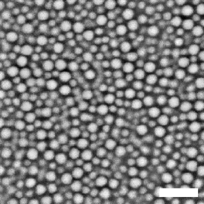
Within each three-dimensional image, we identify both large and small particles. This is accomplished with a single convolution that identifies spherical, bright regions ⁴⁷; the convolution kernel is a three-dimensional Gaussian with a width chosen to match the size of the image of a large particle. Each local maximum after the convolution is identified as a particle ⁴⁷. The distribution of particle brightnesses is bimodal with little overlap, and so small and large particles can be easily distinguished. Our method is the same as is often used to measure particle positions in two dimensions, which normally achieves sub-pixel resolution in particle positions ⁴⁷. However, given that a single convolution kernel is used to identify both particle types, when applied to our binary samples we do not achieve sub-pixel accuracy. Instead, our uncertainty in locating particle positions is linked to the pixel size and is 0.2 $\mu$m in $x$ and $y$, and 0.3 $\mu$m in $z$. We do have accurate discrimination between large and small particles with this method, with less than 1% of the particles misidentified, checked by visual inspection. For a few particles, it is hard to distinguish if they are large or small (because they are small but unusually bright, or large but unusually dim). These particles are assigned to the size that they appear to be the majority of the time.

After identifying the particle positions, they are tracked using standard software ^{47, 46}. The key requirement is that particles move less between time steps than their interparticle spacing, which is easily satisfied in our dense glassy samples. We take images once every 10 - 150 s, depending on the volume fraction, in each case making sure that the acquisition rate is sufficiently rapid to capture all particle movements.

3 Results and Discussion

3.1 Structural characteristics

We begin by looking at the structure of the binary sample. Shown in Fig. 2 is the pair correlation function $g(r)$ of a sample with volume fraction $\phi=0.57$. $g(r)$ relates to the likelihood of finding a particle a distance $r$ away from a reference particle. The three curves correspond to small-small, small-large, and large-large particle pairs, and their first peak positions are at approximately $2a_{S}=2.36$ $\mu$m, $a_{S}+a_{L}=2.73$ $\mu$m, and $2a_{L}=3.10$ $\mu$m. The first peaks of the three curves are fairly broad due to the uncertainty in locating particle positions, and also in part due to the particle polydispersity.

Fig.  2: The pair correlation function $g(r)$ for a sample with volume fraction $\phi=0.57$. The different curves are for small-small pairs, small-large pairs, and large-large pairs, as indicated. Due to particle tracking uncertainties ($\pm 0.2$ $\mu$m in $x$ and $y$, $\pm 0.3$ $\mu$m in $z$), the measured separation $r$ between any pairs of particles has an uncertainty of $\pm 0.5$ $\mu$m, which significantly broadens the peaks of $g(r)$ and diminishes their height.

3.2 Dynamical slowing

We wish to show how the motion of particles slows as the volume fraction increases and approaches the glass transition. Figure 3 shows results of the mean square displacement (MSD) $\langle\Delta{\vec{r}_{i}}^{2}\rangle$ of large and small particles, where $\Delta\vec{r}_{i}=\Delta\vec{r}_{i}(\Delta t)$ denotes the displacement of $i$-th particle in lag time $\Delta t$, and the brackets indicate an average over all particles and times observed. Figure 3 shows that as the volume fraction increases, particle motion slows significantly, as expected. At $\phi=0.4$, small particles take tens of seconds to move a distance $a_{S}^{2}=1.4$ $\mu$m²; at $\phi=0.54$ the time has grown to more than $10^{4}$ s. For the lowest volume fraction samples, comparing the two particle species, we find that $\langle\Delta r^{2}_{S}\rangle/\langle\Delta r^{2}_{L}\rangle\approx a_{L}/a_{S}$, as expected from the Stokes-Einstein-Sutherland equation ^{48, 49}.

As the volume fraction increases, the MSD plots show a characteristic “cage trapping” plateau. Particles cannot diffuse freely, but instead are “caged” by their nearest neighbor particles ^{50, 51, 52, 34, 53, 54}. The upturn in the MSD curve is identified with rearrangements of the cage, allowing the particle to move to a new location, perhaps caged by different particles. Although the smaller particles diffuse faster than the large particles, MSD curves for both show upturns at similar time scales, indicating that their dynamics are strongly coupled ³³. Note that the height of the plateaus (0.1 - 0.2 $\mu$m²) are larger than in prior work ²⁰, because of the larger particle tracking noise present in this binary experiment as compared to the prior work with monodisperse particles. The noise results in apparent displacements $\langle\Delta x^{2}\rangle=\langle\Delta y^{2}\rangle=(0.2$ $\mu$m)², independent of $\Delta t$, and so the minimum reliable value for Fig. 3 is limited to $\sim 0.08$ $\mu$m². In particular the difference between the $\phi=0.58$ and $\phi=0.66$ data is probably not significant, but due to higher tracking errors for the higher volume fraction data. The noise prohibits careful analysis of the mean square displacement data along the lines of prior work ^{55, 56}.

Fig.  3: (Color online) A log-log plot of mean square displacement versus time lag for large particles (a) and small particles (b). Note that our resolution means we cannot accurately measure mean square displacement values less than 0.1 $\mu$m², and thus the plateau height of curves for the highest volume fraction data is set by this limit, rather than the dynamics. However, the slight upturn for those curves at large values of $\Delta t$ is above our resolution limit and thus real. Due to noise in $\langle\Delta z^{2}\rangle$, the data shown are $\langle\Delta x^{2}+\Delta y^{2}\rangle$.

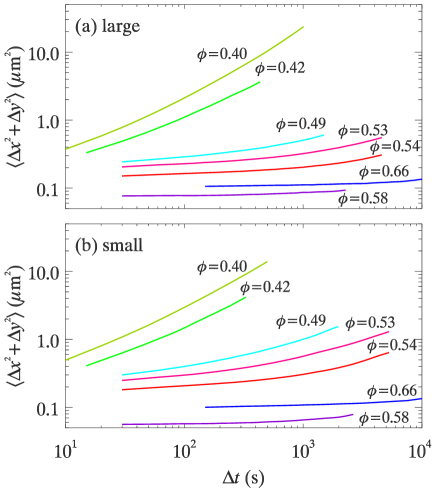
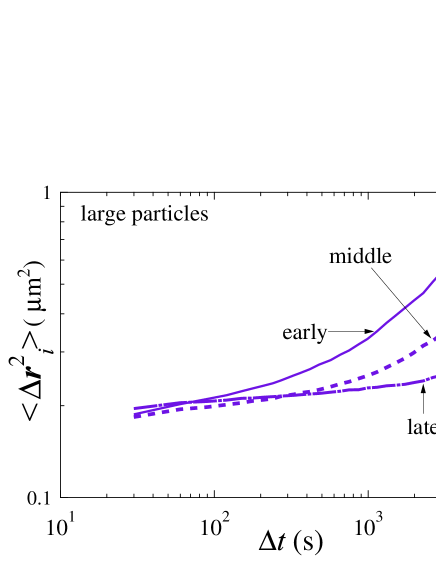
For the samples with $\phi\geq\phi_{g}\approx 0.58$, the MSD curves are nearly flat, suggesting that on our experimental time scales, these samples behave as glasses. Glasses are fundamentally non-equilibrium systems, so that physical properties for glasses depend on the preparation history in general and, in particular, the time since they were initially formed. This time-dependence is known as aging, and can be quantified by examining the MSD at different times since the start of the experiment ^{22, 26, 33}. Figure 4 shows MSD data from $\phi=0.59$. The trajectory data are broken into three equal duration segments and the MSD calculated within each segment; for the older segments, the MSD curve decreases in height (see the caption for details). The sample is most active immediately after being formed, and continues to slow down as time elapses. The aging of the MSD appears in samples for $\phi\geq 0.59$, while no samples for $\phi\leq 0.58$ show aging. From the onset of aging, we conclude that the glass transition point is at volume fraction $\phi\approx 0.59$, similar to that seen for monodisperse samples ⁷. Note that our particle size uncertainty of $\pm 0.02$ $\mu$m (radius) leads to a systematic volume fraction uncertainty, so our estimate is $\phi_{g}=0.59\pm 0.02$ as a comparison with other work.

Fig.  4: (Color online) MSD plot for the large particles from a $\phi=0.59$ sample. The three curves correspond to time regimes with $0<t<4800$ s, $4800<t<9600$ s, and $9600<t<14400$ s. Note that in the first time regime, the sample ages appreciably, so the “early” mean square displacement data should be interpreted with caution. The time-dependence of $\langle\Delta r^{2}\rangle$ is clearly seen, indicating the presence of aging. As $\phi=0.59$ is the lowest volume fraction in which this behavior is seen, we conclude that the glass transition occurs at $\phi_{g}\approx 0.58$. Due to noise in $\langle\Delta z^{2}\rangle$, the data shown are $\langle\Delta r^{2}\rangle=\langle\Delta x^{2}+\Delta y^{2}\rangle$.

Particles involved in a cage rearrangement event move significant distances compared to when they are caged, and prior work noted that the distribution of displacements is unusually broad on the time scale of the rearrangement ^{34, 57}. This is quantified by calculating the non-Gaussian parameter $\alpha_{2}(\Delta t)$, which for a one-dimensional distribution of displacements is defined as

$$\alpha_{2}(\Delta t)=\frac{\langle\Delta x^{4}\rangle}{3\langle\Delta x^{2}\rangle}-1,$$ (1)

where $\Delta x=x(t+\Delta t)-x(t)$ denotes the $x$ displacement for time lag $\Delta t$ ⁵⁸, and the angle brackets indicate an average over all particles and all initial times $t$. If the distribution of displacements $\Delta x$ is Gaussian, then $\alpha_{2}=0$ by construction. If events with large displacements are more common than would be expected from a Gaussian distribution, then $\alpha_{2}>0$. Figure 5 shows the results of the non-Gaussian parameter (NGP) for one-dimension displacements of large and small particles. The curves peak at time scales where cage rearrangements are most important ^{6, 20}, and thus coincides with the upturn of the MSD curves.

$\alpha_{2}$ is fairly sensitive to experimental noise, although fortunately the “signal” this parameter measures comes from particles moving large distances, which are less susceptible to particle position uncertainty. The differences between the data shown in Fig. 5 and the data of Ref. ²⁰ are probably more due to noise and uncertainties in measuring $\phi$, rather than systematic differences between our binary experiments and the prior monodisperse experiments ²⁰. The peak heights of $\alpha_{2}$ for our small particles are similar to those seen in Ref. ²⁰, for roughly similar volume fractions. One notable difference is that Ref. ²⁰ found that for glassy samples, $\alpha_{2}$ started high (1 - 2) and decreased steadily, whereas in our current data, $\alpha_{2}$ remains fairly small for all $\Delta t$, with unclear dependence on $\Delta t$. This is probably due to our noise, as for glassy samples, few particles move distances large enough to be outside of our particle tracking uncertainty.

Fig.  5: (Color online) A semi-log plot of the non-Gaussian parameter $\alpha_{2}$ versus lag time for large particles (a) and small particles (b). The curves for $\phi=0.40,0.42$ are essentially indistinguishable.

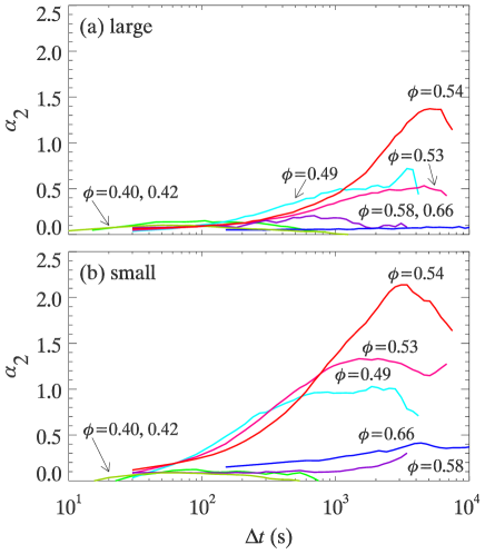
Figure 5 also reveals that the motions of the small particles are more dynamically heterogeneous, with the maximum NGP peaking above 1.5 for the small species but only reaching 0.8 for the large species. This is consistent with recent observations of aging binary colloidal glasses, which likewise found the small particles had more non-Gaussian motion ³³.

From Figs. 3 and 5 we conclude that the dynamics of the large and small particles are qualitatively the same, although with small quantitative differences. In particular, the time scale over which particles escape cages is the same for both, as is the time of peak non-Gaussianity. In much of the subsequent analysis, therefore, we consider both species together in order to obtain better statistical validity.

3.3 Local environment influences mobility

We wish to understand the origins of dynamical heterogeneity. For a hard-sphere system, or an overdamped system such as our experimental colloidal suspension, the only variable is the local structure. Clearly structure has some relation with particle mobility ^{36, 37}, although this relationship may be difficult to see and not directly predictive in nature ³⁵. Prior work found that more disordered environments are weakly correlated with higher particle mobility ^{34, 26}, and a recent study of aging binary colloidal glasses found a relation between the local composition and the mobility ³³.

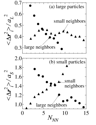
We quantify a particle’s local environment by counting its nearest neighbors $N_{NN}$, defined as particles closer than the first minimum of the pair correlation function for the large particles, 4.1 $\mu$m (Fig. 2), and distinguish between large and small neighbors. Figure 6 shows that the number of neighbors of a given type has a strong influence on the mobility of a particle. Particles with more large neighbors have, on average, a lower mobility, while those with more small neighbors a larger mobility. These observations agree with studies of aging in binary colloidal glasses, ³³ and are reminiscent of prior rheological observations of binary suspensions ^{59, 60, 61} which noted that binary mixtures have lower viscosities than single-component samples with equivalent total volume fraction. The reasoning is that binary suspensions can in general be packed to higher volume fractions, and so have more free volume than monodisperse samples at the same volume fraction. Figure 6 suggests that the small particles indeed “lubricate” large particles, as previously proposed ⁶¹. Conversely, large neighbors significantly inhibit the motion of both large and small particles. The lubricant effect for large particles (which have less free volume) is less pronounced, agreeing with prior observations of monodisperse suspensions which found that regions of mobility correlated with regions of larger free volume ³⁴.

Fig.  6: Large particle mobility as a function of the number of large and small nearest neighbors $N_{NN}$. The panel (b) shows small particle mobility. Mobility is very sensitive to the number of large neighbors, decreasing sharply as the number of large neighbors increases. The number of smaller neighbors has a weaker, yet measurable, impact. These data are for volume fraction $\phi=0.53$, using a time scale $\Delta t=3780$ s to define displacements.

3.4 Cooperative motions

Prior work has shown that the higher mobility molecules in a supercooled liquid are distributed in a spatially heterogeneous fashion ^{5, 6}. In monodisperse colloidal systems, direct imaging using microscopy found that particles rearrange in cooperative groups ^{18, 20, 19}. Following the prior work, we characterize the cooperative nature of colloidal rearrangements by studying the dynamics over a time scale $\Delta t^{*}$ that corresponds to the maximum of the NGP ^{6, 20}. The maximum displacement of a particle over that time $D_{i}$ is defined as

$$D_{i}(t):=\max_{t,t+\Delta t^{*}}(|\vec{r}_{i}(t_{2})-\vec{r}_{i}(t_{1})|)$$ (2)

where $\max_{t,t+\Delta t^{*}}(X)$ is the maximum value of $X$ using times $t_{1}$, $t_{2}$ such that $t\leq t_{1}<t_{2}\leq t+\Delta t^{*}$. Taking the maximum displacement results in a quantity that is less sensitive to random Brownian motion than the ordinary displacement $\Delta r$. Following prior work, ^{6, 20} a threshold $D^{*}(\phi)$ is chosen such that on average, 5% of the particles at any given time have $D_{i}(t)>D^{*}$. These particles are termed “mobile particles” and generally are the ones undergoing cage rearrangements. (Note that at any particular time, the fraction of particles matching this definition is not required to be 5% ⁴⁶.)

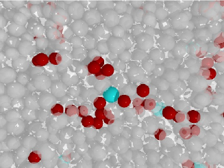
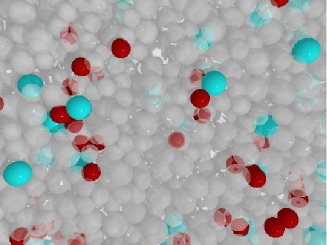
Figure 7 shows snapshots of our system, highlighting the mobile particles. Clusters of these mobile particles are visible, in agreement with previous work which found similar mobile regions ^{6, 20, 33}. The clusters are somewhat smaller than those seen previously in single-component colloidal suspension ²⁰; apparently the dynamics in binary mixtures are less spatially heterogeneous. Our result is in agreement with the results of a simulation study for polydisperse hard-disk systems ⁶², which found that polydispersity reduces dynamic heterogeneity. It is also apparent in Fig. 7 that the small particles dominate the motions for the lower volume fraction (top, $\phi=0.54$) whereas the two species contribute more equally in the glassy sample (bottom, $\phi=0.66$).

Fig.  7: (Color online) Snapshots of system for $\phi=0.54$ (upper) and $\phi=0.66$ (bottom). The red (dark gray) spheres are small mobile particles, and the blue (light gray) spheres are large mobile particles. Mobile particles are defined as those making the largest displacements at this particular moment in time; see text for further details. We set the time lag for the displacement as the cage breaking time scale (the peak time of the NGP $t_{\text{NGP}}$) which is $\Delta t^{*}=3000$ s for $\phi=0.54$ and $t^{*}=4000$ s for $\phi=0.66$.

3.5 Length scales of spatial dynamical heterogeneity

Pictures such as Fig. 7 are qualitative evidence of dynamical heterogeneity. For quantitative information, we consider the vector and scalar spatial-temporal correlation functions ⁴¹ $S_{vec}(R,\Delta t)$ and $S_{scl}(R,\Delta t)$ defined as

$$S_{vec}(R,\Delta t) := \frac{\left<\Delta\vec{r}_{i}\cdot\Delta\vec{r}_{j}\right>_{\text{pair}}}{\left<\Delta\vec{r}^{2}\right>}$$ (3)

$$S_{scl}(R,\Delta t) := \frac{\left<\delta r_{i}\delta r_{j}\right>_{\text{pair}}}{\left<(\delta r)^{2}\right>}.$$ (4)

The vector function $S_{vec}(R,\Delta t)$ characterizes correlations in the vector displacements $\Delta\vec{r}_{i}=\vec{r}_{i}(t+\Delta t)-\vec{r}_{i}(t)$; the similar function $S_{scl}(R,\Delta t)$ uses the scalar displacement $\delta r_{i}=|\Delta\vec{r}_{i}|-\left<|\Delta\vec{r}_{i}|\right>$. The angle brackets $\langle\rangle$ denote an average over all particle pairs with separation $R$ at initial time $t$ as well as an average over $t$. The denominators of both correlation functions are averaged over all particles and time, and do not depend on $R$. The correlation function defined by eqn (3) indicates a vector correlation, and that defined by eqn (4) a scalar correlation. If particles correlate perfectly, the correlation functions are unity. These correlation functions give information about spatial correlations for fixed lag time $\Delta t$, and about temporal dependence of the correlations for fixed separation $R$. We calculate these functions for all pairs of particles, without concern for the particle sizes, both to improve our statistics and because we do not find significant differences for large and small particles only. Most of the “signal” of correlated motion comes from the particles undergoing larger than average displacements, and so the results are less sensitive to the particle tracking uncertainties than the mean square displacement.

Fig.  8: (Color online) Plot of the correlation functions in which the distance $R_{0}=a_{S}+a_{L}=2.73$ $\mu$m is set at the sum of the particle radii. (a) represents the vector correlation [eqn (3)], and (b) the scalar correlation [eqn (4)].

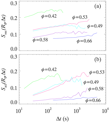
Figure 8 shows the lag time dependence of these correlation functions, in which the distance $R$ is set as the first peak distance of the small-large pair correlation function $g(r)$ (the solid line in Fig. 2). At time scales larger than those shown in Fig. 8, the results become too uncertain, due to lack of data. In intermediate volume fraction region ($\phi<\phi_{g}$), both correlation functions increase with $\Delta t$. For the two lowest volume fractions ($\phi=0.42,0.49$), the correlation functions eventually decrease at large $\Delta t$, but our data do not extend to large enough $\Delta t$ to see this for higher volume fractions. Overall, in conjunction with Fig. 3, Fig. 8 suggests that larger motions are more correlated with the motions of their neighboring particles. This agrees with prior experiments ^{20, 42}. The amplitude of the correlation decreases as $\phi$ increases, with the exception of the $\phi=0.49,0.53$ data which are similar.

For glassy samples ($\phi>0.6$) the correlation functions are small, suggesting that there is little correlation of the motion of neighbors. This is both because there is little overall motion in glassy samples (see Fig. 3) and also the motion that does occur is dominated by Brownian motion within the cage, which is less correlated that the motions responsible for cage rearrangements ³⁴. Furthermore, it is probably erroneous to even consider time-averaged correlation functions for glassy samples, as in this current work the dynamics slow with time (Fig. 4), and so a time average is of dubious validity. (Earlier work studied well-aged samples where the dynamics were only slow aging, and thus a time average was more sensible ⁴².)

Fig.  9: Semi-log plot of the spatial correlation functions of $\phi=0.53$, where the time lag is set as $\Delta t_{\text{NGP}}=2000$s. The solid line is $S_{vec}(R,t_{\text{NGP}})$ and the dashed line is $S_{scl}(R,t_{\text{NGP}})$. The dotted line represents an exponential function with a decay length of 5.8 $\mu$m, a good fit to both functions in this particular case.

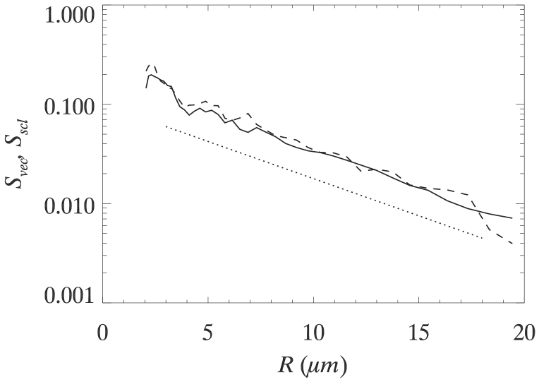
To consider the spatial dynamical heterogeneities, we plot the correlation functions as a function of $R$ in Fig. 9 (for $\phi=0.54$; results for other volume fractions are similar). For small separations around $R=3.5$ $\mu$m, there is a dip in the correlation functions, which corresponds to the dip in the small-large pair correlation function at the same position (solid line in Fig. 2); the peak around $R=2.8$ $\mu$m likewise corresponds to the peak of the small-large pair correlation function. Thus, a particle’s motion is correlated with that of its nearest neighbors, while particles separated by a less structurally favorable distance are less likely to have correlated motion.

We fit our data with an exponential function $S\simeq A\exp(-R/\xi)$ and extract the decay length $\xi$. Figure 10 shows both the vector (triangles) and scalar (circles) decay lengths as a function of the volume fraction. The length scales are essentially constant until close to $\phi_{g}\approx 0.58$, when they show a sharp increase. Our data are too noisy to draw conclusions about how the length scales grow near $\phi_{g}$, although simulations of binary Lennard-Jones mixtures did not find a divergence ⁶³. The largest length scale seen is $\approx 10$ $\mu$m $\approx 8a_{S}\approx 6.5a_{L}$, similar to prior studies of monodisperse colloids ⁴². For $\phi>\phi_{g}$, the scalar length seems large and the vector length decreases, although as noted above, the data should be treated with caution as the samples are aging.

Fig.  10: (Color online) The relationship between the length scales and the volume fraction. Shown are the length scales for the vector correlation function (open triangles) and the scalar correlation function (closed circles). The symbols indicate the average value, and the error bars show the range of values found for different lag times $\Delta t$. These length scales are extracted from the correlation function for all particles (large + small).

3.6 Temporal dynamical heterogeneity

The prior subsection showed that the motion of colloidal particles in our dense samples are spatially heterogeneous. We now study their temporal heterogeneity, using the four-point susceptibility $\chi_{4}$ which measures the correlation in dynamics between any two points in space within some time window ^{43, 45}. The actual value of $\chi_{4}$ is a measure of the average number of particles whose dynamics are correlated, which in turn relates back to the spatial heterogeneity ¹⁴.

Fig.  11: (Color online) Surface plot of $\chi_{4}$ for large particles within a sample with $\phi=0.52$.

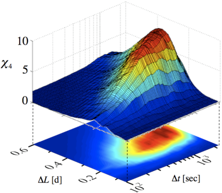
Here we only compute the self contribution to $\chi_{4}$, since it has been shown to be the dominating term ^{43, 45}. The self part is computed from temporal fluctuations in particle mobility, where a particle is defined to be mobile if its displacement over some time interval $\Delta{}t$ is larger than some threshold distance $\Delta{}L$ ⁴⁵. Using this definition, each particle at each time can be labeled mobile or immobile and the fraction of mobile particles $Q(t)$ can be computed for each frame recorded. $Q(t)$ varies from frame to frame due to the spatial heterogeneity. The temporal fluctuations in $Q(t)$ are quantified by the self part to $\chi_{4}$ and written as

$$\chi_{4}=N[\langle Q(t)^{2}\rangle_{t}-\langle Q(t)\rangle_{t}^{2}],$$ (5)

where $N$ is the number of particles. $N$ also varies from frame to frame as particles move in and out of the field of view; we average $N$ over all frames and use $\langle N\rangle$ in eqn (5). (The factor of $N$ arises because the variance scales inversely with particle number.) Note that $\chi_{4}$ measures temporal fluctuations in mobility without regard for the spatial correlations between mobile particles, whereas the correlation functions $S_{vec}$ and $S_{scl}$ studied in the previous section measured spatial correlations of mobility without regard for the temporal correlations. In a sense, then, these two methods of analysis are complementary.

From eqn (5) it’s evident that $\chi_{4}$ will depend on our choice of $\Delta{}L$ and $\Delta{}t$ as shown in Fig. 11, where $\chi_{4}$ is plotted for the larger particles within a $\phi=0.52$ sample for various values of $\Delta{}t$ and $\Delta{}L$. This plot shows that $\chi_{4}$ is characterized by a function that has a maximum at ($\Delta{}t_{\max}$, $\Delta{}L_{\max}$). This maximum in $\chi_{4}$ indicates a typical timescale $\Delta{}t_{\max}$ where the dynamics are most heterogeneous, and likewise $\Delta L_{\max}$ indicates a typical length scale distinguishing caged motions from cage rearrangements.

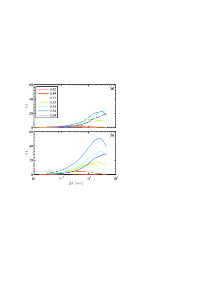
Figure 12 shows plots of $\chi_{4}(\Delta{}t,\Delta{}L=\Delta{}L_{\max})$ for the larger (a) and smaller (b) particles. The value of $\chi_{4}$ is larger in magnitude for the smaller particles regardless of $\phi$, demonstrating that the dynamics of the smaller particles are more temporally heterogeneous. Prior work by Lynch et al. ³³ showed a similar relative mobility; our results build upon this by showing that smaller particles also experience larger fluctuations, and thus exhibit more anomalous spatial and temporal behavior. We also see that $\chi_{4}$ grows in amplitude as $\phi$ increases, but then drops for the glassy sample ($\phi=0.59$), matching the results of the prior subsections where changes were seen at the glass transition.

The plots in Fig. 12 all show a maximum in $\chi_{4}$ at a well defined $\Delta{}t_{\max}$, and that $\Delta{}t_{\max}$ for the various volume fractions occur at timescales close to where $\alpha_{2}$ shows a maximum in Fig. 5 and caging rearrangements become prominent (the “knee” in Fig. 3). The coincidence of maxima in $\chi_{4}$ and $\alpha_{2}$ suggests that local cage rearrangements are the largest contributor to the temporal fluctuations. Since small particles show larger fluctuations, we infer that they may be largely responsible for facilitating local rearrangements, in agreement with the findings of Lynch et al. ³³.

Fig.  12: (Color online) (a) is a plot of the susceptibility of large particles for various packing fractions, and (b) is a plot of the susceptibility of small particles for various packing fractions.

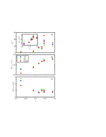
$\chi_{4}^{\max}$, $\Delta{}t_{\max}$, and $\Delta L_{\max}$ all vary with $\phi$; this dependence is shown in Fig. 13. Both $\chi_{4}^{\max}$ and $\Delta{}t_{\max}$ show an increase with $\phi$ illustrating that upon approaching the glass transition the dynamic heterogeneity and the associated time scale increases. The increasing time scale also suggests that local rearrangements take longer at higher $\phi$, in agreement with the extended plateau at higher $\phi$ in Fig. 3. The characteristic length scale $\Delta L$ decreases. This is in excellent agreement with prior work, which showed that the displacements for cage rearrangements are smaller as the glass transition is approached ³⁴. In other words, it requires a smaller displacement to be an anomalously mobile particle. This can also be seen by comparing Figs. 3 and 5: for samples with larger $\phi$, the mean square displacement has a smaller value even when the non-Gaussian parameter is large, showing that the distribution of displacements is overall narrower despite the relatively large fraction of larger-than-expected displacements.

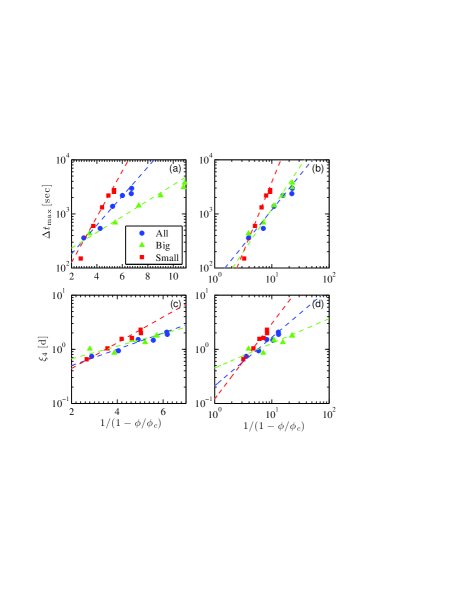
Using the $\chi_{4}^{\max}$ data in Fig. 13(a) a correlation length scale can be estimated by assuming that the correlations $\chi_{4}$ measures are correlated particles forming compact clusters. Since $\chi_{4}$ is the average number of correlated particles, then $\chi_{4}^{\max}=(4/3)\pi\xi_{4}^{3}$, where $\xi_{4}$ is the radius of the cluster of correlated particles in units of particle diameters $d$ ^{45, 64}. The inset in Fig. 13(a) shows the dependence of $\xi_{4}$ on $\phi$. Similarly as with the relaxation time, we see a tendency in $\xi_{4}$ to increase with $\phi$. The growth in $\xi_{4}$ is about a factor of 4 when the volume fraction is increased from a liquid to a dense supercooled state. Our values of $\xi_{4}$ are roughly the same as those measured in a 2D fluidized granular bed on approaching the jamming point ⁴⁵. When compared to $\xi$ shown in Fig. 10 the diameter of these correlated clusters 2$\xi_{4}$ is roughly the same size.

Fig.  13: (Color online) (a) Plot of the maximum of $\chi_{4}$ as a function of $\phi$, showing how temporal heterogeneity increases as $\phi\rightarrow\phi_{g}\approx 0.58$. The inset in (a) shows the dependence of the dynamic heterogeneity length scale $\xi_{4}=(\chi_{4}^{\rm max})^{1/3}$ on $\phi$. (b) Plot of the dynamic heterogeneity time scale as a function of $\phi$. (c) Plot of the length scale $\Delta L$ as a function of $\phi$. For all panels, the symbols are as indicated in the legend of panel (b).

The time scales $\Delta{}t_{\max}$ are analogous to the $\alpha$ relaxation time scales measured in molecular supercooled liquids. In many cases the $\alpha$ relaxation time scales are well described using either a Vogel-Fulcher-Tammann (VFT) model or Mode-Coupling Theory (MCT).

The first model, VFT, predicts that the time scales should obey the form

$$\Delta{}t_{\max}=\Delta{}t_{0}\exp(E/(1-\phi/\phi_{0})),$$ (6)

where $\Delta{}t_{0}$, $E$, and $\phi_{0}$ are all fitting parameters. In the model $\Delta{}t_{0}$ is an attempt time to undergo relaxation events over some typical length scale. For our experiment, this length scale would be on the order of a particle diameter and the attempt time would be the time it takes a particle to diffuse over this length scale in the dilute limit. Using the Stokes-Einstein-Sutherland formula and a viscosity of $2.18$ mPa$\cdot$s (measured for the fluid in absence of colloids) we estimate that at room temperature it should take the small particles about 11 seconds and the large particles 25 seconds to diffuse their own diameter ^{48, 49}. The fitting parameter $\phi_{0}$ is the packing fraction at which diffusive motion should cease. This should occur at random close packing of $\phi\sim 0.65$ (using the value appropriate for our binary suspension). However, as pointed out by Brambilla et. al ¹⁴, there is a debate as to whether the divergence predicted by VFT should occur at the jamming point or at a slightly different packing fraction. To definitively show if this is the case one would need very careful measurements extremely close to the jamming point which is beyond the scope of this paper. The final fitting parameter is $E$, the fragility, which is a material dependent value. The fragility is a measure of how sensitive the time scale is to small changes in volume fraction. For a molecular system $E$ measures how sensitive the relaxation time is to small changes in temperature, and $E$ ranges between $\approx$ 1-100. Materials with low $E$ values are termed fragile glass formers and those with large $E$ values termed strong glass formers ¹.

Fig.  14: (Color online) (a) Log-linear and (b) log-log plots of temporal dynamical heterogeneity time scale, with fits to eqn (6) in panel (a) and eqn (7) in panel (b). (c) Log-linear and (d) log-log plots of the $\chi_{4}$ length scales, with fits to eqn (6) in panel (c) and eqn (7) in panel (d).

The second model, MCT, predicts a scaling of

$$\Delta{}t_{\max}=\Delta{}t_{0}(1-\phi/\phi_{c})^{\gamma},$$ (7)

where $\Delta{}t_{0}$, $\gamma$, and $\phi_{c}$ are the fitting parameters ⁶⁵. $\phi_{c}$ in this model takes a different meaning with the divergence predicted to occur near the glass transition volume fraction, not at random close packing. In light scattering experiments performed by Brambilla et. al on 10% polydisperse colloidal samples they found $\phi_{c}\approx 0.59$, slightly above the glass transition volume fraction ¹⁴. Their work also showed that near the divergence point the dynamics deviate from the predicted form, but that in the supercooled regime the MCT equation describes the data well. They also found a scaling exponent of $\gamma=2.5\pm 0.1$.

Table 1: This table displays the fitting parameters found when fitting the data to either a VFT scaling or a power law scaling. The uncertainties of the fitting parameters are found by adjusting the fitting parameters until they no longer provide reasonable fits.

VFT:	$\Delta{}t_{0}$ [sec] or $\xi_{4}^{0}$ [d]	$E$	$\phi_{0}$
All $\Delta{}t_{\max}$	$70\pm 50$	$0.6\pm 0.3$	$0.64\pm 0.03$
Big $\Delta{}t_{\max}$	$200\pm 160$	$0.4\pm 0.2$	$0.6\pm 0.03$
Small $\Delta{}t_{\max}$	$25\pm 20$	$0.4\pm 0.35$	$0.67\pm 0.03$
All $\xi_{4}$	$0.3\pm 0.2$	$0.4\pm 0.2$	$0.65\pm 0.05$
Big $\xi_{4}$	$0.5\pm 0.2$	$0.3\pm 0.2$	$0.66\pm 0.07$
Small $\xi_{4}$	$0.2\pm 0.15$	$1.0\pm 0.8$	$0.68\pm 0.07$
Power law:	$\Delta{}t_{0}$ [sec] or $\xi_{4}^{0}$ [d]	$\gamma$ or $\delta$	$\phi_{c}$
All $\Delta{}t_{\max}$	$100\pm 90$	$1.3\pm 0.6$	$0.57\pm 0.02$
Big $\Delta{}t_{\max}$	$90\pm 70$	$1.6\pm 0.8$	$0.57\pm 0.02$
Small $\Delta{}t_{\max}$	$20\pm 10$	$2.6\pm 0.9$	$0.61\pm 0.01$
All $\xi_{4}$	$0.2\pm 0.1$	$0.9\pm 0.4$	$0.59\pm 0.03$
Big $\xi_{4}$	$0.5\pm 0.1$	$1.4\pm 0.5$	$0.62\pm 0.04$
Small $\xi_{4}$	$0.15\pm 0.05$	$0.4\pm 0.2$	$0.57\pm 0.02$

Fits to the measured time scales using the two fitting models are shown in Fig. 14(a) and (b), and the corresponding fitting parameters are shown in Table 1. In the previous paragraphs reasonable fitting values were given for some of the different fitting parameters. The $\Delta t_{0}$ values are significantly larger than the dilute concentration diffusive time scales, for both the VFT and MCT fits, although the agreement is off by only a factor of two for the small particles (25 s for VFT, 20 s for MCT, and $\tau_{D}=11$ s). For the VFT fit, $\phi_{c}$ is near $\phi_{rcp}$ as predicted. For the MCT fit $\phi_{c}$ is near the expected glass transition volume fraction of $\approx$ 0.58. The MCT exponent $\gamma$ is smaller than that found by Brambilla et. al ¹⁴, who found $\gamma=2.5$, with the exception of the small particles for which we find $\gamma=2.6\pm 0.9$.

Our data gives fragilities on the order of 0.5, consistent with fragility values from a study of a 2D fluidized granular bed ⁴⁵. When compared to a molecular system our colloidal system would be considered a very fragile glass former.

In the study on the motion of grains in a 2D fluidized granular bed it was shown that the length scales can also be fitted well to the models used to fit the time scales where the VFT formula becomes $\xi_{4}=\xi_{4}^{0}\exp(E/(1-\phi/\phi_{c}))$ and the MCT formula becomes $\xi_{4}=\xi_{4}^{0}(1-\phi/\phi_{c})^{\delta}$, where $\delta$ in work by Berthier et. al is predicted to be 2/3 ^{66, 67}. The work of Brambilla et. al found that $\delta=2/3$ fitted their light scattering data very well ¹⁴.

The fits to the length scales are shown in Fig. 14(c) and (d), and the fitting values are shown in Table 1. The fitting values found for the VFT fits are physically feasible where the fragilities and divergence points compare well to the fitting parameters previously found for the VFT fits to the time scales. The MCT fits are also reasonable, although our scaling exponents $\delta$ is only consistent with the predicted value of 2/3 due to our large error bars. The MCT divergence at $\phi_{c}$ is close to $\phi_{g}$, as expected.

With the range of volume fractions presented in this paper we can not conclusively show which model fits better. Both models capture and predict the time and length scales associated with dynamic heterogeneity, and the derived fitting parameters of both compare well to expected values.

4 Summary

We have used confocal microscopy to study three-dimensional motion of particles in binary colloidal mixture. The volume fraction $\phi$ is varied from 0.4-0.7 and a glass transition, characterized by aging dynamics, is found at $\phi\approx 0.58$. The dynamics of large and small particles are qualitatively similar. At volume fractions approaching the glass transition, both show an increase in motion at the same characteristic cage breaking time scale. This time scale also corresponds with the time over which the displacement distribution functions are broadest (most non-Gaussian). Particle motion is facilitated by the presence of small neighbors, and inhibited by large neighbors, consistent with the idea that small particles serve as lubricants. We have investigated vector and scalar correlation functions and extracted specific length scales associated with the spatial decay in correlation of the displacements. This length slightly increases with volume fraction, although it does not appear to diverge as the glass transition is approached. The temporal correlations also give rise to length scales and time scales which grow as the glass transition is approached, although the form of this growth is ambiguous with respect to power-law or exponential growth.

The presence of particle tracking noise makes certain measurements more difficult, in particular, the pair correlation functions (Fig. 2) and the mean square displacement (Fig. 3). The primary conclusions of our work, however, focus on the particles that move large distances, and these measurements have a “signal” (the distance moved) larger than the “noise” (the instantaneous positional uncertainty). Our measurements of the non-Gaussian parameter (Fig. 5, spatial correlation functions (Figs. 8,9), correlation lengths (Fig. 10, and dynamic susceptibility measurements (Figs. 11 - 14) are robust to the noise. Likewise, the identification of nearest neighbors is fairly robust to even moderate fluctuations in pair-wise particle separations, and so we have confidence in our data showing that having fewer large neighbors enhances a particle’s mobility (Fig. 6).

5 Acknowledgments

We thank the Soft Condensed Matter Group of the Physics Department in Emory University for discussions, in particular J. M. Lynch and G. C. Cianci. T. N. was supported by the 21st Century COE Program “International COE of Flow Dynamics” of Tohoku University. S.V.F. was supported by the National Science Foundation under Grant No. DMR-0239109, and E. R. W. was supported by the NSF under Grant No. CHE-0910707. We thank A. Schofield and W. C. K. Poon for providing our colloidal samples.

References

- Angell 1995 C. A. Angell, Science, 1995, 267, 1924–1935.
- Stillinger 1995 F. H. Stillinger, Science, 1995, 267, 1935–1939.
- Angell et al. 2000 C. A. Angell, K. L. Ngai, G. B. McKenna, P. F. McMillan and S. W. Martin, J. App. Phys., 2000, 88, 3113–3157.
- Adam and Gibbs 1965 G. Adam and J. H. Gibbs, J. Chem. Phys., 1965, 43, 139–146.
- Ediger 2000 M. D. Ediger, Annu. Rev. Phys. Chem., 2000, 51, 99–128.
- Donati et al. 1998 C. Donati, J. F. Douglas, W. Kob, S. J. Plimpton, P. H. Poole and S. C. Glotzer, Phys. Rev. Lett., 1998, 80, 2338–2341.
- Pusey and van Megen 1986 P. N. Pusey and W. van Megen, Nature, 1986, 320, 340–342.
- van Megen and Pusey 1991 W. van Megen and P. N. Pusey, Phys. Rev. A, 1991, 43, 5429–5441.
- Segrè et al. 1995 P. N. Segrè, S. P. Meeker, P. N. Pusey and W. C. K. Poon, Phys. Rev. Lett., 1995, 75, 958–961.
- Cheng et al. 2002 Z. Cheng, J. Zhu, P. M. Chaikin, S.-E. Phan and W. B. Russel, Phys. Rev. E, 2002, 65, 041405.
- Mason and Weitz 1995 T. G. Mason and D. A. Weitz, Phys. Rev. Lett., 1995, 75, 2770–2773.
- Bartsch 1995 E. Bartsch, J. Non-Cryst. Solids, 1995, 192-193, 384–392.
- van Megen et al. 1998 W. van Megen, T. C. Mortensen, S. R. Williams and J. Müller, Phys. Rev. E, 1998, 58, 6073–6085.
- Brambilla et al. 2009 G. Brambilla, D. E. M. El Masri, M. Pierno, L. Berthier, L. Cipelletti, G. Petekidis and A. B. Schofield, Phys. Rev. Lett., 2009, 102, 085703.
- van Megen and Williams 2010 W. van Megen and S. R. Williams, Phys. Rev. Lett., 2010, 104, 169601.
- Brambilla et al. 2010 G. Brambilla, D. E. Masri, M. Pierno, L. Berthier, L. Cipelletti, G. Petekidis and A. Schofield, Phys. Rev. Lett., 2010, 104, 169602.
- van Blaaderen and Wiltzius 1995 A. van Blaaderen and P. Wiltzius, Science, 1995, 270, 1177–1179.
- Marcus et al. 1999 A. H. Marcus, J. Schofield and S. A. Rice, Phys. Rev. E, 1999, 60, 5725–5736.
- Kegel and van Blaaderen 2000 W. K. Kegel and A. van Blaaderen, Science, 2000, 287, 290–293.
- Weeks et al. 2000 E. R. Weeks, J. C. Crocker, A. C. Levitt, A. Schofield and D. A. Weitz, Science, 2000, 287, 627–631.
- König et al. 2005 H. König, R. Hund, K. Zahn and G. Maret, Euro. Phys. J. E, 2005, 18, 287–293.
- Courtland and Weeks 2003 R. E. Courtland and E. R. Weeks, J. Phys.: Cond. Matt., 2003, 15, S359–S365.
- Cipelletti et al. 2003 L. Cipelletti, H. Bissig, V. Trappe, P. Ballesta and S. Mazoyer, J. Phys.: Condens. Matter, 2003, 15, S257–S262.
- Simeonova and Kegel 2004 N. B. Simeonova and W. K. Kegel, Phys. Rev. Lett., 2004, 93, 035701.
- El Masri et al. 2005 D. El Masri, M. Pierno, L. Berthier and L. Cipelletti, J. Phys.: Cond. Matt., 2005, 17, S3543–S3549.
- Cianci et al. 2006 G. C. Cianci, R. E. Courtland and E. R. Weeks, Solid State Comm., 2006, 139, 599–604.
- Yunker et al. 2009 P. Yunker, Z. Zhang, K. Aptowicz and A. Yodh, Phys. Rev. Lett., 2009, 103, 115701.
- Nugent et al. 2007 C. R. Nugent, K. V. Edmond, H. N. Patel and E. R. Weeks, Phys. Rev. Lett., 2007, 99, 025702.
- Sarangapani and Zhu 2008 P. S. Sarangapani and Y. Zhu, Phys. Rev. E, 2008, 77, 010501.
- Conrad et al. 2006 J. C. Conrad, P. P. Dhillon, E. R. Weeks, D. R. Reichman and D. A. Weitz, Phys. Rev. Lett., 2006, 97, 265701.
- Zhu et al. 1997 J. Zhu, M. Li, R. Rogers, W. Meyer, R. H. Ottewill, Sts-73, W. B. Russel and P. M. Chaikin, Nature, 1997, 387, 883–885.
- Gasser et al. 2001 U. Gasser, E. R. Weeks, A. Schofield, P. N. Pusey and D. A. Weitz, Science, 2001, 292, 258–262.
- Lynch et al. 2008 J. M. Lynch, G. C. Cianci and E. R. Weeks, Phys. Rev. E, 2008, 78, 031410.
- Weeks and Weitz 2002 E. R. Weeks and D. A. Weitz, Phys. Rev. Lett., 2002, 89, 095704.
- Conrad et al. 2005 J. C. Conrad, F. W. Starr and D. A. Weitz, J. Phys. Chem. B, 2005, 109, 21235–21240.
- Widmer-Cooper et al. 2004 A. Widmer-Cooper, P. Harrowell and H. Fynewever, Phys. Rev. Lett., 2004, 93, 135701.
- Widmer-Cooper and Harrowell 2005 A. Widmer-Cooper and P. Harrowell, J. Phys.: Cond. Matt., 2005, 17, S4025–S4034.
- Prasad et al. 2007 V. Prasad, D. Semwogerere and E. R. Weeks, J. Phys.: Cond. Matt., 2007, 19, 113102.
- Poole et al. 1998 P. H. Poole, C. Donati and S. C. Glotzer, Physica A: Statistical and Theoretical Physics, 1998, 261, 51–59.
- Donati et al. 1999 C. Donati, S. C. Glotzer and P. H. Poole, Phys. Rev. Lett., 1999, 82, 5064–5067.
- Doliwa and Heuer 2000 B. Doliwa and A. Heuer, Phys. Rev. E, 2000, 61, 6898–6908.
- Weeks et al. 2007 E. R. Weeks, J. C. Crocker and D. A. Weitz, J. Phys.: Cond. Matt., 2007, 19, 205131.
- Glotzer et al. 2000 S. C. Glotzer, V. N. Novikov and T. B. Schrø der, J. Chem. Phys., 2000, 112, 509–512.
- Lacevic et al. 2003 N. Lacevic, F. W. Starr, T. B. Schroder and S. C. Glotzer, J. Chem. Phys., 2003, 119, 7372–7387.
- Keys et al. 2007 A. S. Keys, A. R. Abate, S. C. Glotzer and D. J. Durian, Nature Physics, 2007, 3, 260–264.
- Dinsmore et al. 2001 A. D. Dinsmore, E. R. Weeks, V. Prasad, A. C. Levitt and D. A. Weitz, App. Optics, 2001, 40, 4152–4159.
- Crocker and Grier 1996 J. C. Crocker and D. G. Grier, J. Colloid Interf. Sci., 1996, 179, 298–310.
- Einstein 1905 A. Einstein, Annalen der Physik (Leipzig), 1905, 17, 549–560.
- Sutherland 1905 W. Sutherland, Phil. Mag., 1905, 9, 781–785.
- Rabani et al. 1997 E. Rabani, D. J. Gezelter and B. J. Berne, J. Chem. Phys., 1997, 107, 6867–6876.
- Doliwa and Heuer 1998 B. Doliwa and A. Heuer, Phys. Rev. Lett., 1998, 80, 4915–4918.
- Kasper et al. 1998 A. Kasper, E. Bartsch and H. Sillescu, Langmuir, 1998, 14, 5004–5010.
- Weeks and Weitz 2002 E. R. Weeks and D. A. Weitz, Chem. Phys., 2002, 284, 361–367.
- Reis et al. 2007 P. M. Reis, R. A. Ingale and M. D. Shattuck, Phys. Rev. Lett., 2007, 98, 188301.
- Ngai and Rendell 1998 K. L. Ngai and R. W. Rendell, Phil. Mag. B, 1998, 77, 621–631.
- van Megen et al. 2009 W. van Megen, V. A. Martinez and G. Bryant, Phys. Rev. Lett., 2009, 102, 168301.
- Kob et al. 1997 W. Kob, C. Donati, S. J. Plimpton, P. H. Poole and S. C. Glotzer, Phys. Rev. Lett., 1997, 79, 2827–2830.
- Rahman 1964 A. Rahman, Phys. Rev., 1964, 136, A405–A411.
- Hoffman 1992 R. L. Hoffman, J. Rheology, 1992, 36, 947–965.
- D’Haene and Mewis 1994 P. D’Haene and J. Mewis, Rheologica Acta, 1994, 33, 165–174.
- Williams and van Megen 2001 S. R. Williams and W. van Megen, Phys. Rev. E, 2001, 64, 041502.
- Kawasaki et al. 2007 T. Kawasaki, T. Araki and H. Tanaka, Phys. Rev. Lett., 2007, 99, 215701.
- Narumi and Tokuyama 2008 T. Narumi and M. Tokuyama, Phil. Mag., 2008, 88, 4169–4175.
- Sarangapani et al. 2008 P. Sarangapani, J. Zhao and Y. Zhu, J. Chem. Phys., 2008, 129, 104514.
- Götze 1999 W. Götze, J. Phys.: Cond. Matt., 1999, 11, A1–A45.
- Berthier et al. 2007 L. Berthier, G. Biroli, J. P. Bouchaud, W. Kob, K. Miyazaki and D. R. Reichman, J. Chem. Phys., 2007, 126, 184503.
- Berthier et al. 2007 L. Berthier, G. Biroli, J. P. Bouchaud, W. Kob, K. Miyazaki and D. R. Reichman, J. Chem. Phys., 2007, 126, 184504.