Probing dark energy with future redshift surveys: A comparison of emission line and broad band selection in the near infrared

Abstract

Future galaxy surveys will map the galaxy distribution in the redshift interval $0.5<z<2$ using near-infrared cameras and spectrographs. The primary science goal of such surveys is to constrain the nature of the dark energy by measuring the large-scale structure of the Universe. This requires a tracer of the underlying dark matter which maximizes the useful volume of the survey. We investigate two potential survey selection methods: an emission line sample based on the $\mathrm{H}\alpha$ line and a sample selected in the H-band. We present predictions for the abundance and clustering of such galaxies, using two published versions of the GALFORM galaxy formation model. Our models predict that $\mathrm{H}\alpha$ selected galaxies tend to avoid massive dark matter haloes and instead trace the surrounding filamentary structure; H-band selected galaxies, on the other hand, are found in the highest mass haloes. This has implications for the measurement of the rate at which fluctuations grow due to gravitational instability. We use mock catalogues to compare the effective volumes sampled by a range of survey configurations. To give just two examples: a redshift survey down to $H_{\rm AB}=22$ samples an effective volume that is $\sim 5-10$ times larger than that probed by an $\mathrm{H}\alpha$ survey with $\mbox{${\rm log}(F_{H\alpha}\mbox{$[\mathrm{erg}\ \mathrm{s}^{-1}\ \mathrm{cm}^{-2}]$})$}>-15.4$; a flux limit of at least $\mbox{${\rm log}(F_{H\alpha}\mbox{$[\mathrm{erg}\ \mathrm{s}^{-1}\ \mathrm{cm}^{-2}]$})$}=-16$ is required for an $\mathrm{H}\alpha$ sample to become competitive in effective volume.

1 Introduction

A number of approaches have been proposed to uncover the nature of the accelerating expansion of the Universe which involve measuring the large scale distribution of galaxies (e.g Albrecht et al., 2006; Peacock et al., 2006). The ability of galaxy surveys to discriminate between competing models depends on their volume. Once the solid angle of a survey has been set, the useful volume can be maximised by choosing a tracer of the large-scale structure of the Universe which can effectively probe the geometrical volume. This depends on how the abundance of tracers drops with increasing redshift, and how much of this decline is offset by an increase in the clustering amplitude of the objects.

Several wide-angle surveys have probed the redshift interval between $0<z<1$ (e.g Colless et al., 2003; York et al., 2000; Cannon et al., 2006; Blake et al., 2009). The next major step up in volume will be made when the range from $0.5<z<2$ is opened up with large near-infrared cameras and spectrographs which are mounted on telescopes able to map solid angles running into thousands of square degrees. From the ground, this part of the electromagnetic spectrum is heavily absorbed by water vapour in the Earth’s atmosphere and affected by the strong atmospheric OH emission lines. A space mission to construct an all-sky map of galaxies in the redshift range $0.5<z<2$ would have a significant advantage over a ground based survey in that the sky background in the near-infrared (NIR) is around 500 times weaker in space than it is on the ground.

An important issue yet to be resolved for a galaxy survey extending to $z\sim 2$ is the construction of the sample and the method by which the redshifts will be measured. One option is to use slitless spectroscopy and target the $\mathrm{H}\alpha$ emission line. $\mathrm{H}\alpha$ is located at a restframe wavelength of $\lambda=6563$Å, which, for galaxies at $z>0.5$, falls into the near-infrared part of the electromagnetic spectrum (Thompson et al., 1996; McCarthy et al., 1999; Hopkins et al., 2000; Shim et al., 2009). $\mathrm{H}\alpha$ emission is powered by UV ionizing photons from massive young stars. The only source of attenuation is dust, which is less important at the wavelength of $\mathrm{H}\alpha$ than it is for shorter wavelength lines. This makes $\mathrm{H}\alpha$ a more direct tracer of galaxies which are actively forming stars than other lines such as $\mathrm{Ly}\alpha$, OII, OIII, H$\beta$ or H$\gamma$, which suffer from one or more sources of attenuation (i.e. dust, stellar absorption, resonant scattering) and which are more sensitive to the metallicity and ionisation state of the gas. The second option is to use some form of multi-slit spectrograph to carry out a redshift survey of a magnitude limited sample. The use of a slit means that unwanted background is reduced, allowing fainter galaxies to be targetted. Also, it is easier to identify which spectrum belongs to which galaxy with a slit than it is with slitless spectroscopy. Targets could be selected in the H-band at an effective wavelength of just over 1 micron, which is around the centre of the near infrared wavelength part of the spectrum.

Space missions designed to carry out redshift surveys like the ones outlined above are currently being planned and assessed on both sides of the Atlantic. At the time of writing, the European Space Agency is conducting a Phase A study of a mission proposal called Euclid , one component of which is a galaxy redshift survey. Both of the selection techniques mentioned above are being evaluated as possible spectroscopic solutions. The slit solution for Euclid is based on a novel application of digital micromirror devices (DMDs) to both image the galaxies to build a parent catalogue in the H-band and to measure their redshifts (see Cimatti et al. 2009 for further details about the Euclid redshift survey). A $\mathrm{H}\alpha$ mission is also being discussed in the USA . At this stage, the sensitivity of these missions is uncertain and subject to change. For this reason we consider a range of $\mathrm{H}\alpha$ flux limits and H-band magnitudes when assessing the performance of the surveys. The specifications and performance currently being discussed for these missions have motivated the range of fluxes that we consider.

A simple first impression of the relative merits of different selections methods can be gained by calculating the effective volume of the resulting survey. This requires knowledge of the survey geometry and redshift coverage, along with the redshift evolution of the number density of sources and their clustering strength. In this paper we use published galaxy formation models to predict the abundance and clustering of different samples of galaxies in order to compute the effective volumes of a range of $\mathrm{H}\alpha$ and H-band surveys. Observationally, relatively little is known about the galaxy population selected by $\mathrm{H}\alpha$ emission or H-band magnitude at $0.5<z<2$. Empirically it is possible to estimate the number density of sources from the available luminosity function data and, on adopting a suitable model, to use the limited clustering measurements currently available to infer the evolution of the number density and bias (Shioya et al., 2008; Morioka et al., 2008; Geach et al., 2008). Geach et al. (2009), in a complementary study to this one, make an empirical estimate of the number density of $\mathrm{H}\alpha$ emitters, and combine this with the predictions of the clustering of these galaxies presented in this paper to estimate the efficiency with which $\mathrm{H}\alpha$ emitters can measure the large scale structure of the Universe.

The outline of the paper is as follows: in Section 2 we give a brief overview of the models. Some general properties of $\mathrm{H}\alpha$ emitters in the models, such as luminosity functions (LF), equivalent widths (EW) and clustering bias are presented in Section 3 as these have not been published elsewhere. In Section 4 we show how our models can be used to build mock survey catalogues. We analyse the differences in the clustering of $\mathrm{H}\alpha$ emitters and H-band selected galaxies and present an indication of the efficiency with which different surveys trace large-scale structure (LSS). Finally, we give our conclusions in Section 5.

2 The Models

In this paper we present predictions for the clustering of galaxy samples selected in the near-infrared using two published versions of the semi-analytic model GALFORM. An overview of the semi-analytical approach to modelling galaxy formation can be found in Baugh (2006). The GALFORM code is described in Cole et al. (2000) and Benson et al. (2003). The two models considered in this paper are explained fully in the original papers, Baugh et al. (2005) (hereafter the Bau05  model) and Bower et al. (2006) (hereafter the Bow06 model). A thorough description of the ingredients of the Bau05  model can also be found in Lacey et al. (2008); detailed comparisons of the physical ingredients of the two models are given in Almeida et al. (2007, 2008), Gonzalez et al. (2009) and Gonzalez-Perez et al. (2009). Here we give an overview of the main features of each model and refer the reader to the above references for further details.

The models are used to calculate the properties of the galaxy population as a function of time, starting from the merger histories of dark matter haloes and invoking a set of rules and recipes to describe the baryonic physics. These prescriptions require parameter values to be set to define the model. These values are set by comparing the model predictions against observations of local galaxies. The Bau05 and Bow06 models have many ingredients in common but differ in the way in which they suppress the formation of bright galaxies. Also, different emphasis was placed on reproducing various local datasets when setting the parameters of the two models. It is important to remember that our starting point here is the two “off the shelf” galaxy formation models, which were set up without reference to $\mathrm{H}\alpha$ or H-band observations. In view of this it is remarkable how close these models come to matching the observed $\mathrm{H}\alpha$LFs and H-band counts and redshift distributions, as presented in the next sections.

The Bau05 model uses a superwind to stifle the formation of bright galaxies. The rate of mass ejection is assumed to be proportional to the star formation rate. The superwind ejects baryons from small and intermediate mass haloes. The cooling rate in massive haloes is reduced because these haloes have a reduced baryon fraction, due to the operation of the superwind in their progenitors. The model assumes that star formation which takes place in bursts occurs with a top-heavy initial mass function (IMF). For each solar mass of stars formed, four times the number of Lyman continuum photons are produced in a starburst as would be made in a quiescent episode of star formation, in which stars are produced with a standard solar neighbourhood IMF (Kennicutt, 1983). Highlights of the Bau05  model include matching the observed number counts and redshift distribution of sub-millimetre sources and the luminosity function of Lyman-break galaxies. The Bau05  model also successfully reproduces the abundance and properties (including clustering) of $\mathrm{Ly}\alpha$ emitters (Le Delliou et al., 2005, 2006; Orsi et al., 2008).

The Bow06 model, on the other hand, uses feedback from active galactic nuclei (AGN) to stop the formation of bright galaxies. The accretion of “cooling flow” gas directly onto a central supermassive black hole releases jets of energy which heat the hot gas, and greatly reduces the cooling flow (see Croton et al. 2005). Hence the supply of cooling gas for star formation is switched off. The Bow06  model gives a good match to the bimodal nature of the colour distribution of local galaxies (Gonzalez et al. 2009), to the abundance of red galaxies (Almeida et al. 2007; Gonzalez-Perez et al. 2009) and to the evolution of the stellar mass function (Bower et al. 2006).

Figure 1: The $\mathrm{H}\alpha$ luminosity function, including attenuation by dust, at different redshifts. The blue curves show the predictions of the Bau05  model, whereas red curves show the Bow06  model. The observational estimates are represented by the symbols (see text for details). The redshift displayed in the bottom-right corner of each panel gives the redshift at which the GALFORM models were run. The vertical black dashed line shows the $\mathrm{H}\alpha$ luminosity corresponding to the flux $\mbox{${\rm log}(F_{H\alpha}\mbox{$[\mathrm{erg}\ \mathrm{s}^{-1}\ \mathrm{cm}^{-2}]$})$}=-15.4$ for $z>0$, displayed to show the expected luminosity limit of current planned space missions.

Other differences between the two models include: i) starbursts triggered by dynamically unstable disks in the Bow06  model; ii) a universal solar neighbourhood IMF in the Bow06  model; iii) the use of dark matter halo merger histories extracted from an N-body simulation in the Bow06 model, whereas the Bau05 model uses Monte-Carlo generated trees; iv) a slightly different set of cosmological parameters ($\mbox{$\Omega_{\rm{m}}$}=0.3$, $\mbox{$\Omega_{\rm{\Lambda}}$}=0.7$, $\Omega_{b}=0.04$, $h=0.7$, $\sigma_{8}=0.9$ for the Bau05 model, and $\mbox{$\Omega_{\rm{m}}$}=0.25$, $\mbox{$\Omega_{\rm{\Lambda}}$}=0.75$, $\Omega_{b}=0.045$, $h=0.73$, $\sigma_{8}=0.93$ for the Bow06 model).

The calculation of H-band flux and $\mathrm{H}\alpha$ line emission is the same in both models. The model predicts the star formation history of each galaxy, recording the star formation rate and the metallicity with which stars are made in each of the galaxy’s progenitors. This allows a composite stellar population and spectral energy distribution to be built up. The model predicts the scale size of the galaxy and, through a chemical evolution model, the metal content of the disk and bulge. The H-band magnitude is computed by convolving the model galaxy spectral energy distribution with an H-band filter, appropriately shifted in wavelength if the galaxy is observed at $z>0$. The effect of dust extinction is taken into account by assuming that the dust and disk stars are mixed together (Cole et al. 2000). The spectral energy distribution also gives the rate of production of Lyman continuum photons. Then, all of the ionizing photons are assumed to be absorbed by the neutral gas in the galaxy, and, by adopting case B recombination (Osterbrock 1989), the emissivity of the $\mathrm{H}\alpha$ line (and other emission lines) is computed. Here we assume that the attenuation of the $\mathrm{H}\alpha$ emission is the same as that experienced by the continuum at the wavelength of $\mathrm{H}\alpha$ . To predict the equivalent width (EW) of the $\mathrm{H}\alpha$ emission, we simply divide the luminosity of the line by the luminosity of the continuum around the $\mathrm{H}\alpha$ line.

3 Properties of $\mathrm{H}\alpha$ emitters

We first concentrate on the nature of $\mathrm{H}\alpha$ emitters in the models, which have not been discussed elsewhere for GALFORM , before examining the clustering of $\mathrm{H}\alpha$ and H-band selected samples in more detail in the next section. In this section we present the basic predictions for the abundance, equivalent width distributions and clustering of $\mathrm{H}\alpha$ emitters. Note that all the results presented here include the attenuation of the $\mathrm{H}\alpha$ emission by dust in the ISM at the same level experienced by the continuum at the wavelength of $\mathrm{H}\alpha$ .

3.1 The $\mathrm{H}\alpha$ luminosity function

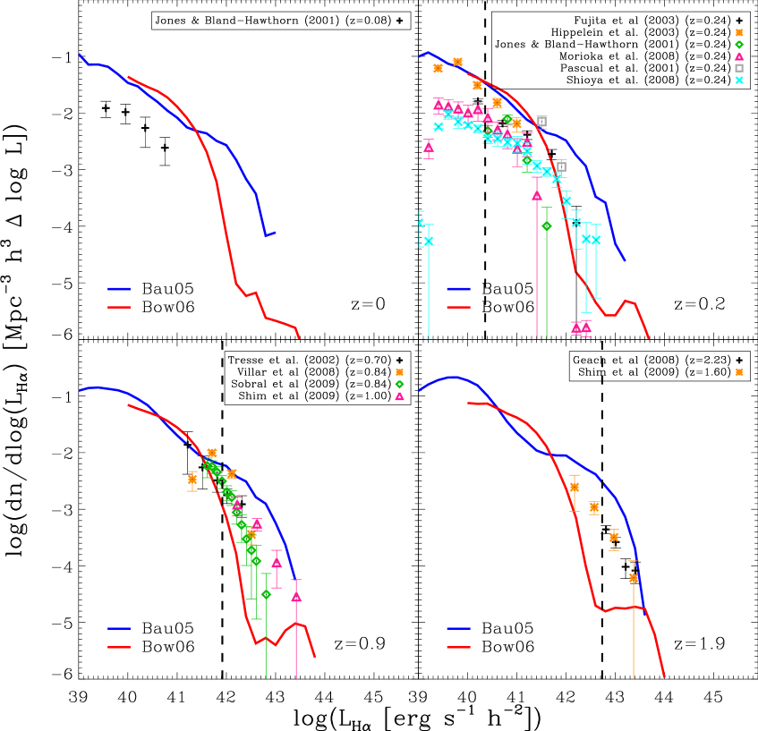
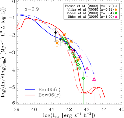
A basic prediction of the models is the evolution of the $\mathrm{H}\alpha$ luminosity function (LF). Fig. 1 shows the $\mathrm{H}\alpha$ LFs predicted by the two versions of GALFORM compared with observational data, over the redshift interval $0<z<2$. At each redshift plotted, the Bau05  model predicts a higher number density of $\mathrm{H}\alpha$ emitters than the Bow06  model for luminosities brighter than $\mbox{${\rm log}(L_{H\alpha}\mbox{$[\mathrm{erg}\ \mathrm{s}^{-1}\ \mathrm{cm}^{-2}]$})$}\simeq 42$. This reflects two processes: the relative efficiency of the feedback mechanisms used in the two models to suppress the formation of bright galaxies, and the top-heavy IMF adopted in starbursts in the Bau05  model, which, for a galaxy with a given star formation rate, boosts the $\mathrm{H}\alpha$ flux emitted. The bright end of the $\mathrm{H}\alpha$ LF is dominated by bursting galaxies.

At faint luminosities, Fig. 1 shows that the predicted model LFs are more similar. At these luminosities, the star formation in both models predominantly takes place in galactic disks and produces stars with a standard IMF. For luminosities fainter than $\mbox{${\rm log}(L_{H\alpha}\mbox{$[\mathrm{erg}\ \mathrm{s}^{-1}\ \mathrm{cm}^{-2}]$})$}\simeq 40$, the Bow06  model suffers from the limited mass resolution of Millennium Simulation halo merger trees (Springel et al. 2005) compared with that of the Monte Carlo trees used in the Bau05  model (Helly et al., 2003).

The observational data shown in Fig. 1 comes from Jones & Bland-Hawthorn (2001) for $z\sim 0$; Fujita et al. (2003),Hippelein et al. (2003) ,Jones & Bland-Hawthorn (2001), Morioka et al. (2008),Pascual et al. (2001),Shioya et al. (2008) for $z\sim 0.2$; Tresse et al. (2002), Villar et al. (2008),Sobral et al. (2009),Shim et al. (2009) for $z\sim 0.9$ and Geach et al. (2008),Shim et al. (2009) for $z=2.2$. Most of this observational data has not been corrected by the authors for dust extinction, and hence it can be directly compared to the GALFORM predictions, which include dust attenuation. However, in some cases the data were originally presented after correction for an assumed constant attenuation. In such cases we have undone this “correction”. Hence, our comparison concerns the actual observed number of $\mathrm{H}\alpha$ emitters, which is the relevant quantity for assessing the performance of a redshift survey.

In general both models overpredict the number of low luminosity $\mathrm{H}\alpha$ emitters at $z\leq 0.3$, as shown by Fig. 1. At $z=0$, (upper-left panel in Fig. 1), the amplitude of the LF in both models is larger, by almost an order of magnitude, than the Jones & Bland-Hawthorn (2001) data. A similar conclusion is reached at $z=0.2$ (upper-right panel in Fig. 1), on comparing the models to most of the observational data. However, there is a significant scatter in observations of the faint end of the LF. At redshifts $z\ga 1$ (bottom panels in Fig. 1), the models bracket the observational estimates, with the Bow06  model tending to underpredict the observational LF, whereas the Bau05  model over predicts it. Despite the imperfect agreement, these model LFs “bracket” the observed LFs for the redshifts relevant to space mission surveys propsed, so we proceed to use them for the purposes of this paper.

Figure 2: The distribution of $\mathrm{H}\alpha$ equivalent width in the observer frame as a function of $\mathrm{H}\alpha$ flux, over the redshift interval $0.7<z<1.9$. The top panel shows the predictions of the Bau05  model and the bottom panel shows the Bow06  model, calculated as described in the text. The black line shows the median EW at each flux. The shaded regions enclose $68\%$ (dark grey) and $95\%$ (light grey) respectively of the GALFORM predictions around the median (black circles). The blue circles show observational data from Hopkins et al. (2000), green asterisks show data from Shim et al. (2009) and red diamonds show data from McCarthy et al. (1999), as indicated by the key. The magenta dashed lines show the GALFORM predictions for the median equivalent width after applying the empirically derived continuum flux and line luminosity rescalings described in Section 4.

3.2 $\mathrm{H}\alpha$ equivalent width (EW) distribution

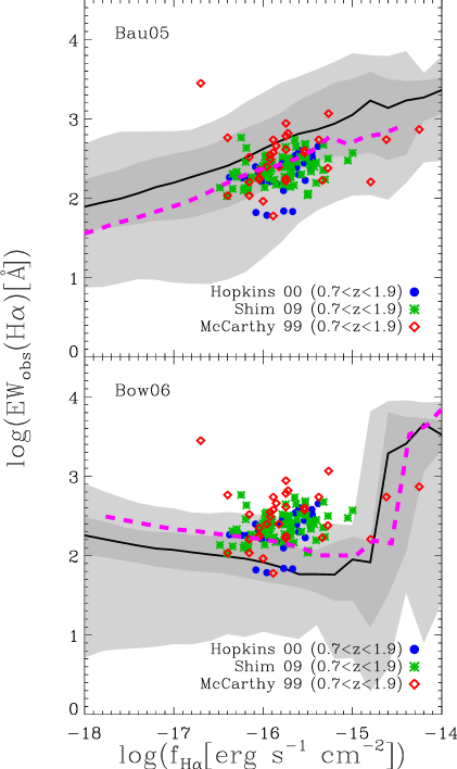
Broadly speaking the EW of the $\mathrm{H}\alpha$ line depends on the current SFR in a galaxy (which determines the $\mathrm{H}\alpha$ emission), and its stellar mass (to which the continuum luminosity is more closely related). We compare the model predictions for the EW of $\mathrm{H}\alpha$ versus $\mathrm{H}\alpha$ flux with observational results in Fig. 2. The observational data cover a wide redshift interval, $0.7<z<1.9$ (McCarthy et al., 1999; Hopkins et al., 2000; Shim et al., 2009). In order to mimic the observational selection when generating model predictions, we go through the following two steps. First, we run the models for a set of redshifts covering the above redshift range. Second, we weight the $EW_{\mathrm{obs}}$ distribution at a given flux by ${\rm d}N/{\rm d}z$, the redshift distribution of $\mathrm{H}\alpha$ emitters over the redshift range, to take into account the change in the volume element between different redshifts (see Section 4 for details of the calculation of ${\rm d}N/{\rm d}z$).

Fig. 2 shows the $EW_{\mathrm{obs}}$ distribution predicted by the Bau05  model (top panel) and the Bow06  model (bottom panel). The models predict different trends of $EW_{\mathrm{obs}}$ with $\mathrm{H}\alpha$ flux. In the Bau05  model, the typical EW increases with $\mathrm{H}\alpha$ flux, with a median value close to $\mbox{$EW_{\mathrm{obs}}$}\sim 100$Å at $\mbox{${\rm log}(F_{H\alpha}\mbox{$[\mathrm{erg}\ \mathrm{s}^{-1}\ \mathrm{cm}^{-2}]$})$}=-18$, reaching $\mbox{$EW_{\mathrm{obs}}$}\sim 2000$Å at $\mbox{${\rm log}(F_{H\alpha}\mbox{$[\mathrm{erg}\ \mathrm{s}^{-1}\ \mathrm{cm}^{-2}]$})$}=-14$. In contrast, the Bow06  model predicts a slight decline of $EW_{\mathrm{obs}}$ with $\mathrm{H}\alpha$ flux until very bright fluxes are reached, with median $\mbox{$EW_{\mathrm{obs}}$}\sim 100$Å in the range $\mbox{${\rm log}(F_{H\alpha}\mbox{$[\mathrm{erg}\ \mathrm{s}^{-1}\ \mathrm{cm}^{-2}]$})$}=[-18,-15]$. For $\mbox{${\rm log}(F_{H\alpha}\mbox{$[\mathrm{erg}\ \mathrm{s}^{-1}\ \mathrm{cm}^{-2}]$})$}>-15$, the Bow06  model predicts a sharp increase of the median $EW_{\mathrm{obs}}$ to $\sim 3000$Å. The $95\%$ interval of the $EW_{\mathrm{obs}}$ found in GALFORM galaxies (the light grey region in Fig. 2) covers almost 2 orders of magnitude in both models, except in the plateau found in the brightest bin of the Bow06  model, where the distribution covers 3 orders of magnitude. The Bau05  model matches the observed distribution of equivalent widths the best, particularly after the rescaling of continuum and line luminosities discussed in the next section (after which the median EW versus $\mathrm{H}\alpha$ distribution shifts from the solid black to the dashed magenta line). It is interesting to note that the “shifted” relations (see §4) give a better match to the observations for both models (although the Bau05  model remains a better fit), particularly as the shift was derived with reference to the H-band galaxy number counts (for the continuum) and to the $z\sim 1$ $\mathrm{H}\alpha$ LF, rather than to the EW data.

Figure 3: The effective bias parameter as a function of $\mathrm{H}\alpha$ luminosity for redshifts spanning the range $0<z<2$. The Bau05  model results are shown using circles connected with solid lines and the Bow06  model results are shown with asterisks connected by dashed lines. Each colour corresponds to a different redshift, as indicated by the key.

3.3 Clustering of $\mathrm{H}\alpha$ emitters: effective bias

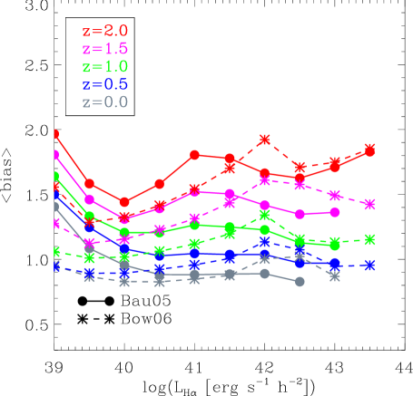
The clustering bias, $b$, is defined as the square root of the ratio of the galaxy correlation function to the correlation function of the dark matter (Kaiser, 1984). As we shall see in Section 4.3, the clustering bias is a direct input into the calculation of the effective volume of a galaxy survey, which quantifies how well the survey can measure the large scale structure of the Universe. Simulations show that the correlation functions of galaxies and dark matter reach an approximately constant ratio on large scales (see for example Angulo et al. 2008a; note, however, that small departures from a constant ratio are apparent even on scales in excess of $100h^{-1}$Mpc).

In this section we compute the effective bias of samples of $\mathrm{H}\alpha$ emitting galaxies. There are theoretical prescriptions for calculating the bias factor of dark matter haloes as a function of mass and redshift (Cole & Kaiser, 1989; Mo & White, 1996; Sheth, Mo & Tormen, 2001). These have been extensively tested against the clustering of haloes measured in N-body simulations and have been found to be reasonably accurate (Gao, Springel & White, 2005; Wechsler et al., 2006; Angulo et al., 2008b). Here we use Sheth, Mo & Tormen (2001). The effective bias is computed by integrating over the halo mass the bias factor corresponding to the dark matter halo which hosts a galaxy multiplied by the abundance of the galaxies of the chosen luminosity (see, for example Baugh et al., 1999; Le Delliou et al., 2006; Orsi et al., 2008).

Model	$C_{H\alpha}$	$C_{\rm cont}$
Bau05	0.35	0.73
Bow06	1.73	0.42

Table 1: Luminosity rescaling factors for the $\mathrm{H}\alpha$ line and the stellar continuum. Column 2 shows $C_{H\alpha}$, the factor used to adjust the predicted $\mathrm{H}\alpha$ flux as described in the text. This factor is only applied to the $\mathrm{H}\alpha$ line. Column 3 shows $C_{cont}$, the correction factor applied to the stellar continuum, as derived by forcing the model to match the observed H-band counts at $H_{\rm AB}=22$. This factor is applied to the entire stellar continuum of the model galaxies.

Fig. 3 shows the predicted galaxy bias, $b_{\rm eff}$, as a function of $\mathrm{H}\alpha$ luminosity over the redshift interval $0<z<2$. There is a clear increase in the value of the effective bias with redshift; at $\mbox{${\rm log}(L_{H\alpha}\mbox{$[\mathrm{erg}\ \mathrm{s}^{-1}\ \mathrm{cm}^{-2}]$})$}=40$, $b_{\rm eff}\approx 0.8$ at $z=0$, compared with $b_{\rm eff}\approx 1.5$ at $z=2$. Both models show an upturn in the effective bias with decreasing luminosity faintwards of $\mbox{${\rm log}(L_{H\alpha}\mbox{$[\mathrm{erg}\ \mathrm{s}^{-1}\ \mathrm{cm}^{-2}]$})$}=40$. There is little dependence of bias on luminosity brightwards of $\mbox{${\rm log}(L_{H\alpha}\mbox{$[\mathrm{erg}\ \mathrm{s}^{-1}\ \mathrm{cm}^{-2}]$})$}=40$, up to $z=2$. The predictions of the two models for the effective bias are quite similar. There are currently few observational measurements of the clustering of $\mathrm{H}\alpha$ emitters. Geach et al. (2008) inferred a spatial correlation length of $r_{0}=4.2^{+0.4}_{-0.2}h^{-1}$Mpc for their sample of 55 $\mathrm{H}\alpha$ emitters at $z=2.23$. This corresponds to a bias of $b\approx 1.7$ in the Bau05  model cosmology, which is in very good agreement with the predictions plotted in Fig. 3.

4 The effectiveness of redshift surveys for measuring dark energy

In this section we assess the relative merits of using $\mathrm{H}\alpha$ or H-band selection to construct future redshift surveys aimed at measuring the dark energy equation of state. The first step is to produce a mock catalogue that can reproduce currently available observations. We discuss how we do this in Section 4.1. We then present predictions for the clustering of $\mathrm{H}\alpha$ emitters and H-band selected galaxies in Section 4.2. We quantify the performance of the two selection methods in terms of how well the resulting surveys can measure the large-scale structure of the Universe in Section 4.3.

4.1 Building accurate mock catalogues

Figure 4: Number counts in the H band. The upper panel shows the differential counts on a log scale. The lower panel shows the counts after dividing by a power law $N_{\rm ref}\propto H_{\rm AB}^{0.32}$ to expand the dynamic range on the y-axis. The symbols show the observational data, as shown by the key in the upper panel. The lines show the model predictions. The dotted lines show the original GALFORM predictions for the Bau05  model (blue) and the Bow06  model (red). The solid curves show the rescaled GALFORM predictions after rescaling the model galaxy luminosities to match the observed number counts at $H_{\rm AB}=22$.

Figure 5: The redshift distribution of galaxies with $H_{\rm AB}=22$ (left column) and $H_{\rm AB}<23$ (right column). The top panels show the predictions after rescaling the model luminosities to better match the number counts as explained in the text. Red and blue lines show the model predictions for $H_{\rm AB}<22$ and $H_{\rm AB}<23$ respectively. Solid lines show the Bau05(r) model and the dashed lines show the Bow06(r) model. The lower panel shows the redshift distribution obtained from the Bow06  model by diluting the galaxies, randomly selecting 0.63 of the sample, the Bow06(d) model (recall this is a purely illustrative case with no physical basis; see §4.1.1). In both panels, the histogram shows an estimate of the redshift distribution derived from spectroscopic observations in the COSMOS and UDF fields (Cirasuolo et al., 2008, ; Euclid-NIS Science Team, private communication).

Our goal in this section is to build mock catalogues for future redshift surveys which agree as closely as possible with currently available observational data. We have already seen that the models are in general agreement with observations of the $\mathrm{H}\alpha$ luminosity function, and will see in the next subsection how well the models match the H-band number counts. In our normal mode of operation, we set the model parameters with reference to a subset of local observations and see how well the model then agrees with other observables. This allows us to test the physics of the model; if the model cannot reproduce a dataset adequately, perhaps some ingredient is missing from the model (e.g. for an application of this principle to galaxy clustering, see Kim et al., 2009). Here our primary aim is not to develop our understanding of galaxy formation physics but to produce a synthetic catalogue which resembles the real Universe as closely as possible. To achieve this end we allow ourselves the freedom to rescale the model stellar continuum and emission line luminosities, independently. This preserves the ranking of the model galaxies in luminosity. This approach is more powerful than an empirical model as we retain all of the additional information predicted by the semi-analytical model, such as the clustering strength of the galaxies. Hereafter we will refer to the adjusted Bau05  and Bow06  models as Bau05(r) and Bow06(r)  respectively, to avoid confusion. We also consider a sparsely sampled version of the Bow06  model, which we refer to as Bow06(d) (see §4.1.1).

4.1.1 H-band selected mock catalogues

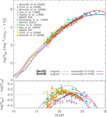
In Fig. 4, we first compare the model predictions without any rescaling of the luminosities against a compilation of observed number counts in the H-band, kindly provided by Nigel Metcalfe. Observational data are taken from the following sources, shown with different symbols: Black plus-signs from Metcalfe et al. (2006); purple asterisks from Frith et al. (2006); purple diamonds from Metcalfe et al. (2006); blue triangles from Yan et al. (1998); blue squares from Teplitz et al. (1998); cyan crosses from the second data release of the 2MASS Survey ; green circles from Thompson et al. (1999); green plus-signs from Martini (2001); green asterisks from Chen et al. (2002); green diamonds from Moy (2003); green triangles from the 2MASS extended source catalogue, orange squares from Frith et al. (2006), and orange triangles from Retzlaff et al. (2009)

Figure 6: The $\mathrm{H}\alpha$ LF at $z=0.9$. The symbols show observational data, with the sources indicated in the key. The dotted curves show the original predictions for the $\mathrm{H}\alpha$ luminosity function, as plotted in Fig. 1. The solid curves show the model predictions after rescaling the $\mathrm{H}\alpha$ luminosity to better match the observed LF at $\mbox{${\rm log}(L_{H\alpha}\mbox{$[\mathrm{erg}\ \mathrm{s}^{-1}\ \mathrm{cm}^{-2}]$})$}=42$, which corresponds to a flux limit of $\mbox{${\rm log}(F_{H\alpha}\mbox{$[\mathrm{erg}\ \mathrm{s}^{-1}\ \mathrm{cm}^{-2}]$})$}=-15.3$ at this redshift.

Figure 7: The redshift distribution of $\mathrm{H}\alpha$ selected galaxies for 3 different flux limits: $\mbox{${\rm log}(F_{H\alpha}\mbox{$[\mathrm{erg}\ \mathrm{s}^{-1}\ \mathrm{cm}^{-2}]$})$}>$ -15.3, -15.7 and -16.0 shown in red, blue and green respectively. The solid lines show the Bau05(r) prediction and the dashed lines show the Bow06(r) predictions. In the top panel, galaxies contributing to the redshift distribution have no cut imposed on the equivalent width of $\mathrm{H}\alpha$ . In the bottom panel, the model galaxies have to satisfy the $\mathrm{H}\alpha$ flux limit and a cut on the observed equivalent width of $\mathrm{H}\alpha$ of $\mbox{$EW_{\mathrm{obs}}$}>100$Å.

There is a factor of three spread in the observed counts around $H_{\rm AB}=20-22$. The unscaled models agree quite well with the observations at $H_{\rm AB}=20$ but overpredict the counts at $H_{\rm AB}=22$, the likely depth of a slit-based redshift survey from space. There are two ways in which the model predictions can be brought into better agreement with the observed counts at $H_{\rm AB}=22$; first, by rescaling the luminosities of the model galaxies to make them fainter in the H-band or second, by artificially reducing, at each magnitude, the number density of galaxies. The first correction could be explained as applying extra dust extinction to the model galaxies; as we will see later on, the typical redshift of the galaxies is $z\sim 0.5$–$1$, shifting the observer frame H into the rest frame R to V-band. The second correction has no physical basis and is equivalent to taking a sparse sampling of the catalogue at random, i.e. making a dilution of the catalogue. Galaxies are removed at random without regard to their size or redshift. (Note that the dissolution of galaxies invoked by Kim et al. 2009 only applies to satellite galaxies within haloes, and is mass dependent, and hence is very different from the random dilution applied here.) The motivation behind the second approach is that the shape of the original redshift distribution of the model is preserved. As we shall see, the first approach, rescaling the model galaxy luminosities, produces a significant change in the shape of the predicted redshift distribution.

It is worth remarking in passing that the semi-analytical models used here have already been compared to the observed counts in the K-band (Gonzalez-Perez et al., 2009). The Bow06  model was found to agree very well with the K-band observations whereas the Bau05  model underpredicted the counts by up to a factor of three. This is a somewhat different impression about the relative merits of the models from that reached on comparing to the observed H-band counts, which is surprising given the proximity of the bands and the similarity in the masses of the stars which dominate the light from the composite stellar populations at these wavelengths.

The agreement with the observed counts is improved at $H_{\rm AB}=22$ by shifting the Bow06  galaxy magnitudes faintwards by $+0.92$ magnitudes; the Bau05  model requires a more modest dimming of $+0.33$ magnitudes (see Table  1).

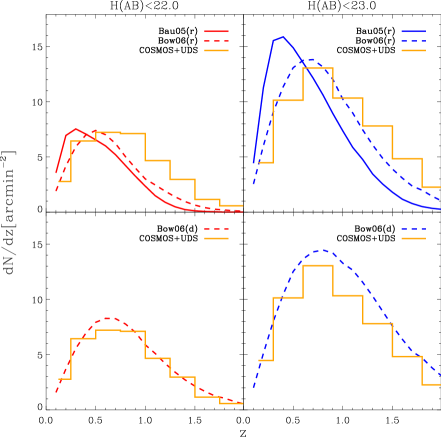
The redshift distribution of H-band selected galaxy samples provides a further test of the models. In Fig. 5, the model predictions are compared against an estimate of the redshift distribution compiled using observations from the COSMOS survey and the Hubble Ultra-Deep Field for $H_{\rm AB}<22$ and $H_{\rm AB}<23$ (Cirasuolo et al. 2008; Cirasuolo, Le Fevre and McCracken, private communication). If we focus on the lower panels first, which shows ${\rm d}N/{\rm d}z$ in the randomly diluted Bow06  model, denoted as Bow06(d), it is apparent that the original Bow06  model predicted the correct shape for the redshift distribution of sources, but with simply too many galaxies at each redshift. In the upper panel of Fig. 5, we see that the models with the shifted H-band luminosities give shallower redshift distributions than the observed one. The difference between the predicted ${\rm d}N/{\rm d}z$ after dimming the luminosities or diluting the number of objects has important implications for the number density of galaxies as a function of redshift, which in turn is important for the performance of a sample in measuring the large-scale structure of the Universe.

4.1.2 $\mathrm{H}\alpha$-selected mock catalogues

The original model predictions for the $\mathrm{H}\alpha$ luminosity function were presented in Fig. 1. The models cross one another and match the observed $\mathrm{H}\alpha$ LF at a luminosity of $\mbox{${\rm log}(L_{H\alpha}\mbox{$[\mathrm{erg}\ \mathrm{s}^{-1}\ \mathrm{cm}^{-2}]$})$}\sim 41.5$. At $z=0.9$, this corresponds to a flux of $\mbox{${\rm log}(F_{H\alpha}\mbox{$[\mathrm{erg}\ \mathrm{s}^{-1}\ \mathrm{cm}^{-2}]$})$}=-15.8$. The flux limit attainable by Euclid is likely to be somewhat brighter than this, although the precise number is still under discussion. For this reason, we chose to force the models to agree with the observed $\mathrm{H}\alpha$ LF at $\mbox{${\rm log}(L_{H\alpha}\mbox{$[\mathrm{erg}\ \mathrm{s}^{-1}\ \mathrm{cm}^{-2}]$})$}=42$ at $z=0.9$, which corresponds to a flux limit of $\mbox{${\rm log}(F_{H\alpha}\mbox{$[\mathrm{erg}\ \mathrm{s}^{-1}\ \mathrm{cm}^{-2}]$})$}=-15.3$ (see Fig. 6). Before rescaling, the model LFs differ by a factor of three at $\mbox{${\rm log}(L_{H\alpha}\mbox{$[\mathrm{erg}\ \mathrm{s}^{-1}\ \mathrm{cm}^{-2}]$})$}\sim 41.5$. In the rescaling, the $\mathrm{H}\alpha$ line luminosity is boosted in the Bow06  model and reduced in the case of the Bau05  model (see Table 1 for the correction factors used in both cases). The latter could be explained as additional dust extinction applied to the emission line, compared with the extinction experienced by the stellar continuum. The former correction, a boost to the $\mathrm{H}\alpha$ luminosity in the Bow06  model, is harder to explain. This would require a boost in the production of Lyman-continuum photons (e.g. as would result on invoking a top-heavy IMF in starbursts or an increase in the star formation rate). This would require a revision to the basic physical ingredients of the model and is beyond the scope of the current paper.

Figure 8: The spatial distribution of galaxies and dark matter in the Bow06(r) model at $z=1$. Dark matter is shown in grey, with the densest regions shown with the brightest shading. Galaxies selected by their $\mathrm{H}\alpha$ emission with $\mbox{${\rm log}(F_{H\alpha}\mbox{$[\mathrm{erg}\ \mathrm{s}^{-1}\ \mathrm{cm}^{-2}]$})$}>-16.00$ and and $\mbox{$EW_{\mathrm{obs}}$}>100$Å are shown in red in the left-hand panels. Galaxies brighter than $H_{\rm AB}=22$ are shown in green in the right-hand panels. Each row shows the same region from the Millennium simulation. The first row shows a slice of $200\mbox{$h^{-1}\mathrm{Mpc}$}$ on a side and $10\mbox{$h^{-1}\mathrm{Mpc}$}$ deep. The second row shows a zoom into a region of $50\mbox{$h^{-1}\mathrm{Mpc}$}$ on a side and $10\mbox{$h^{-1}\mathrm{Mpc}$}$ deep, which corresponds to the white square drawn in the first row images. Note that all of the galaxies which pass the selection criteria are shown in these plots.

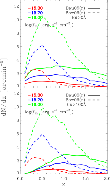
After making this correction to the $\mathrm{H}\alpha$ line flux in the models, we next present the predictions for the redshift distribution of $\mathrm{H}\alpha$ emitters. Fig. 7 shows ${\rm d}N/{\rm d}z$ for flux limits of $\mbox{${\rm log}(F_{H\alpha}\mbox{$[\mathrm{erg}\ \mathrm{s}^{-1}\ \mathrm{cm}^{-2}]$})$}=[-15.7,-16.0,-16.3]$. The redshift distribution of the Bow06(r) model peaks around $z\sim 0.5$ and declines sharply approaching $z\sim 2$, whereas the Bau05(r) ${\rm d}N/{\rm d}z$  are much broader. The lower panel of Fig. 7 shows the redshift distribution after applying the flux limits and a cut on the observed equivalent width of $\mbox{$EW_{\mathrm{obs}}$}=100$Å. (Note that the ${\rm d}N/{\rm d}z$ is not sensitive to low EW cuts; similar results to the $\mbox{$EW_{\mathrm{obs}}$}>0$ Å case are obtained with 10Å in both models). In the rescaled model, the equivalent width changes because the $\mathrm{H}\alpha$ line flux has been adjusted and because the continuum has been altered (by the same shift as applied to the H-band). Adding the selection on equivalent width results in a modest change to the predicted ${\rm d}N/{\rm d}z$ in the Bow06(r) model. In the Bau05(r) model, the ${\rm d}N/{\rm d}z$ shifts to higher redshifts. There is no observational data on the redshift distribution of $\mathrm{H}\alpha$ emitters to compare against the model predictions. Geach et al. (2009) make an empirical estimate of the redshift distribution, by fitting a model for the evolution of the luminosity function to observational data. The luminosity of the characteristic break in the luminosity function, $L_{*}$, is allowed to vary, while the faint end slope and normalisation are held fixed. The resulting empirical LF looks similar to the original Bau05 model at $z=0.9$, and the two have similar redshift distributions. The $\mathrm{H}\alpha$ redshift distributions in the Bow06(r) models are shallower than the empirical estimate; the Bau05(r) model has a similar shape to the empirical redshift distribution, but with a lower normalisation. It is important to realise that the approach of Geach et al. is also model dependent, and the choices of model for the evolution of the luminosity function and of which observational datasets to match are not unique and will have an impact on the resulting form of the redshift distribution.

4.2 The clustering of $\mathrm{H}\alpha$ and H-band selected samples

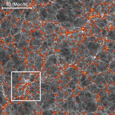
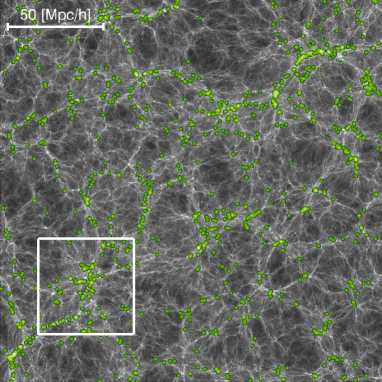
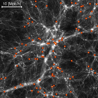
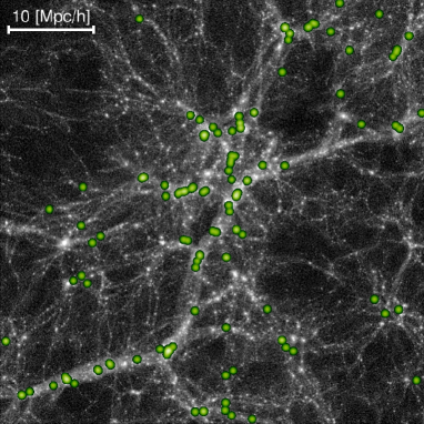
The semi-analytic galaxy formation model predicts the number of galaxies hosted by dark matter haloes of different mass. In the cases of $\mathrm{H}\alpha$ emission, which is primarily sensitive to ongoing star formation, and H-band light, which depends more on the number of long-lived stars, different physical processes determine the number of galaxies per halo. The model predicts contrasting spatial distributions for galaxies selected according to their $\mathrm{H}\alpha$ emission or H-band flux. We compare in Fig. 8 the spatial distribution of $\mathrm{H}\alpha$ emitters with fluxes $\mbox{${\rm log}(F_{H\alpha}\mbox{$[\mathrm{erg}\ \mathrm{s}^{-1}\ \mathrm{cm}^{-2}]$})$}>-16$ and $\mbox{$EW_{\mathrm{obs}}$}>100$Å (red circles) with that of an H-band selected sample with $H_{\rm AB}<22$ (green circles), in the Bow06(r) model which is set in the Millennium Simulation. The upper panels of Fig. 8 show how the different galaxy samples trace the underlying cosmic web of dark matter. The lower panels of Fig. 8 show a zoom into a massive supercluster. There is a marked difference in how the galaxies trace the dark matter on these scales. The $\mathrm{H}\alpha$ emitters avoid the most massive dark matter structures. At the centre of massive haloes, the gas cooling rate is suppressed in the model due to AGN heating of the hot halo. This reduces the supply of gas for star formation and in turn cuts the rate of production of Lyman continuum photons, and hence the $\mathrm{H}\alpha$ emission. The H-band selected galaxies, on the other hand, sample the highest mass dark matter structures.

To study the difference in the spatial distribution of galaxies in a quantitative way, we compare the clustering predictions from the models with observational data. Instead of computing the correlation function explicitly, we use the same method explained in Section 3.3 to calculate the effective bias and use this to derive the correlation length, $r_{0}$, a measure of the clustering amplitude, which we define as the pair separation at which the correlation function equals unity. The correlation function of galaxies, $\xi_{\rm gal}$, is related to the correlation function of dark matter, $\xi_{\rm dm}$, by $\xi_{\rm gal}=b^{2}\xi_{\rm dm}$. The effective bias is approximately constant on large scales (e.g. Angulo et al. 2008a). We use the Smith et al. (2003) prescription to generate a nonlinear matter power spectrum in real space. This in turn is Fourier transformed to obtain the two-point correlation function of the dark matter, $\xi_{\rm dm}$. We can then derive $\xi_{\rm gal}$ for any survey configuration by multiplying $\xi_{\rm dm}$ by the square of the effective bias, and then we read off the correlation length as the scale at which the correlation function is equal to unity.

Figure 9: The correlation length, $r_{0}$, as a function of redshift for selected $\mathrm{H}\alpha$ and H-band samples. Solid and dashed lines show the predictions of the Bau05  and Bow06  models respectively. The top panel shows the predictions for different $\mathrm{H}\alpha$ limiting fluxes, $\mbox{${\rm log}(F_{H\alpha}\mbox{$[\mathrm{erg}\ \mathrm{s}^{-1}\ \mathrm{cm}^{-2}]$})$}>[-16.0,-16.5,-17.0]$ in green, orange and blue respectively. Observational data is shown with symbols. The bottom panel shows the model predictions for $H_{AB}<[20.,20.5]$ in orange and blue respectively. In this case there are two sets of observational estimates, based on different assumptions for the evolution of clustering with redshift.

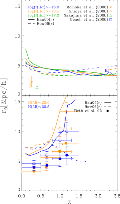
Fig. 9 shows the correlation length in comoving units for both $\mathrm{H}\alpha$ and H-band samples at different redshifts, compared to observational estimates. Differences in the bias predicted by the two models (as shown in Fig. 3) translate into similar differences in $r_{0}$. The correlation length declines with increasing redshift for $\mathrm{H}\alpha$ emitters in the Bau05(r) model, since the increase of the effective bias with redshift is not strong enough to balance the decline of the amplitude of clustering of the dark matter. For the range of flux limits shown in the top panel of Fig. 9 ($-16<\mbox{${\rm log}(F_{H\alpha}\mbox{$[\mathrm{erg}\ \mathrm{s}^{-1}\ \mathrm{cm}^{-2}]$})$}<-17$), $r_{0}$ changes from $\sim 5-7\ \mbox{$h^{-1}\mathrm{Mpc}$}$ at $z=0.1$ to $r_{0}\sim 3.5\ \mbox{$h^{-1}\mathrm{Mpc}$}$ at $z=2.5$. On the other hand, the Bow06(r) model shows a smooth increase of $r_{0}$ which depends on flux and redshift. At bright flux limits $r_{0}$ evolves rapidly at high redshift, reaching $r_{0}=4.3h^{-1}$Mpc at $z=2.5$. At fainter luminosities the change in correlation length with redshift is weaker.

The currently available observational estimates of the clustering of near infrared selected galaxy samples mainly come from angular clustering. A number of assumptions are required in order to derive a spatial correlation length from the angular correlation function. First, a form must be adopted for the distribution of sources in redshift. Second, some papers quote results in terms of proper separation whereas others report in comoving units. Lastly, an evolutionary form is sometimes assumed for the correlation function (Groth & Peebles, 1977). In this case, the results obtained for the correlation length depend upon the choice of evolutionary model.

Estimates of the correlation length of $\mathrm{H}\alpha$ emitters are available at a small number of redshifts from narrow band surveys, as shown in Fig. 9 (Morioka et al., 2008; Shioya et al., 2008; Nakajima et al., 2008; Geach et al., 2008). These surveys are small and sampling variance is not always included in the error bar quoted on the correlation length (see Orsi et al. 2008 for an illustration of how sampling variance can affect measurements of the correlation function made from small fields). The models are in reasonable agreement with the estimate by Geach et al. (2008) at $z=2.2$, but overpredict the low redshift measurements. The $z=0.24$ measurements are particularly challenging to reproduce. The correlation length of the dark matter in the $\Lambda$CDM model is around $5h^{-1}$Mpc at this redshift, so the $z=0.24$ result implies an effective bias of $b<0.5$. Gao & White (2007) show that dark matter haloes at the resolution limit of the Millennium Simulation, $M\sim 10^{10}h^{-1}M_{\odot}$, do not reach this level of bias, unless the 20% of the youngest haloes of this mass are selected. In the Bow06(r) model, the $\mathrm{H}\alpha$ emitters populate a range of halo masses, with a spread in formation times, and so the effective bias is closer to unity. Another possible explanation for the discrepancy is that the observational sample could be contaminated by objects which are not $\mathrm{H}\alpha$ emitters and which dilute the clustering signal.

The bottom panel of Fig. 9 shows the correlation length evolution for different H-band selections, compared to observational estimates from Firth et al. (2002). Note that the samples analysed by Firth et al. are significantly brighter than the typical samples considered in this paper ($H_{\rm AB}=20$ versus $H_{\rm AB}=22$). Firth et al. use photometric redshifts to isolate galaxies in redshift bins before measuring the angular clustering. Two sets of observational estimates are shown for each magnitude limit, corresponding to two choices for the assumed evolution of clustering. Again the models display somewhat stronger clustering than the observations would suggest at low redshift. The Bau05(r) model predicts a clustering length which increases with redshift. The Bow06(r) model, on the other hand, predicts a peak in the correlation length around $z\sim 0.7$, with a decline to higher redshifts. This reflects the form of the luminosity - halo mass relation for galaxy formation models with AGN feedback (Kim et al., 2009). The slope of the luminosity - mass relation changes at the mass for which AGN heating becomes important. Coupled with the appreciable scatter in the predicted relation, this can result in the brightest galaxies residing in haloes of intermediate mass.

Figure 10: The two point correlation function, measured in redshift space, plotted in bins of pair separation parallel ($r_{\pi}$) and perpendicular ($r_{\sigma}$) to the line of sight, $\xi(r_{\sigma},r_{\pi})$, for $\mathrm{H}\alpha$ emitters (left-hand panels) and H-band selected (right-hand panels) galaxies in the Millennium simulation. The samples used are those plotted in Fig. 8. The pair counts are replicated over the four quadrants to enhance the visual impression of deviations from circular symmetry. The $\mathrm{H}\alpha$ catalogue has a limiting flux of $\mbox{${\rm log}(F_{H\alpha}\mbox{$[\mathrm{erg}\ \mathrm{s}^{-1}\ \mathrm{cm}^{-2}]$})$}>-16$ and an equivalent width cut of $\mbox{$EW_{\mathrm{obs}}$}>100$Å; the H-band magnitude limit is $H_{\rm AB}=22$. The contours show where ${\rm log}(\mbox{$\xi(r_{\sigma},r_{\pi})$})=[0.5,0.0,-0.5,-1.0,-1.5]$, from small to large pair separations. The upper panels show the correlation function measured in fully sampled catalogues without redshift errors. The middle panels show how redshift errors change the clustering pattern. Representative errors for the two redshift measurements are used: $\sigma_{z}=10^{-3}$ for the slitless case ($\mathrm{H}\alpha$ emitters), and $\sigma_{z}=2\times 10^{-4}$ for the slit based measurement (H-band selected). In the upper and middle panels, all the galaxies are used to compute the correlation function. In the bottom panels, only 33% of the galaxies are used in each case, which is indicative of the likely redshift success rate for a survey from space.

4.3 Redshift-space distortions

The amplitude of gravitationally induced bulk flows is sensitive to the rate at which perturbations grow, which depends on the expansion history of the universe and the nature of the dark energy (Wang, 2008; Guzzo et al., 2008). Bulk flows can be measured by their impact on the correlation function of galaxies when plotted as a function of pair separation perpendicular and parallel to the line of sight, $\xi(r_{\sigma},r_{\pi})$ (Hawkins et al., 2003; Ross et al., 2007). We now restrict our attention to the Bow06(r) model, since this is set in the Millennium Simulation and we can measure the clustering of the model galaxies directly. As the Millennium simulation has periodic boundary conditions, we can estimate the correlation function as follows:

$$\xi(r_{\sigma},r_{\pi}) = \frac{DD_{\sigma,\pi}}{N\bar{n}\Delta V_{\sigma,\pi}}-1,$$ (1)

$$\Delta V_{\sigma,\pi} = 2\pi r_{\sigma}\Delta r_{\sigma}\Delta r_{\pi},$$ (2)

where $DD_{\sigma,\pi}$ is the number of distinct galaxy pairs in a bin of pair separation centred on $(r_{\sigma},r_{\pi})$, $\Delta r_{\sigma}$ and $\Delta r_{\pi}$ are the widths of the bins in the $r_{\sigma}$ and $r_{\pi}$ directions, respectively, $N$ and $\bar{n}$ are the total number of galaxies and the number density of galaxies in the sample, and $\Delta V_{r_{\sigma},r_{\pi}}$ corresponds to the volume enclosed in an annulus centred on $(r_{\sigma},r_{\pi})$. Note that to avoid any confusion, here we refer to the line of sight separation as $r_{\pi}$ and use $\pi$ to denote the mathematical constant.

In redshift surveys, the radial distance to a galaxy is inferred from its redshift. The measured redshift contains a contribution from the expansion of the Universe, along with a peculiar velocity which is induced by inhomogeneties in the density field around the galaxy. Thus the position inferred from the redshift is not necessarily the true position. The distortion of the clustering pattern resulting from peculiar velocities is referred to as the redshift space distortion. On large scales, coherent motions of galaxies from voids towards overdense regions lead to a boost in the clustering amplitude (Kaiser, 1987):

$$\frac{\xi(s)}{\xi(r)}=1+\frac{2}{3}\beta+\frac{1}{5}\beta^{2},$$ (3)

where $\xi(s)$ is the spherically averaged, redshift space correlation function, and $\xi(r)$ is its equivalent in real space (i.e. without the contribution of peculiar velocities). Eq. (3) holds in linear perturbation theory in the distant observer approximation when gradients in the bulk flow and the effect of the velocity dispersion are small (Cole et al., 1994; Scoccimarro, 2004). Strictly speaking, these approximations apply better on large scales. The parameter $\beta$ is related to the linear growth rate, $D$, through

$$\beta_{\rm lin} = \frac{1}{b}\frac{{\rm d}\ln D}{{\rm d}\ln a},$$ (4)

$$\approx \frac{\mbox{$\Omega_{\rm{m}}$}(z)^{\gamma}}{b},$$ (5)

where $a$ is the expansion factor. The approximation in Eq. (5) is valid for an open cosmology, in which $\gamma$ is traditionally approximated to $0.6$ (Peebles, 1980). Lahav et al. (1991) showed that this approximation should be modified in the case of a CDM model with a cosmological constant, to display a weak dependence on $\Lambda$. Lue, Scoccimarro & Starkman (2004) pointed out that the value of $\gamma$ allows one to differentiate between modified gravity and dark energy, since $\beta(z)\simeq\Omega_{m}(a)^{2/3}/b$ for DGP gravity models, while $\beta(z)\simeq\Omega_{m}(a)^{5/9}/b$ for a flat Universe with a cosmological constant.

On small scales, the randomised motions of galaxies inside virialised structures lead to a damping of the redshift space correlation function and a drop in the ratio $\xi(s)/\xi(r)$(Cole et al., 1994).

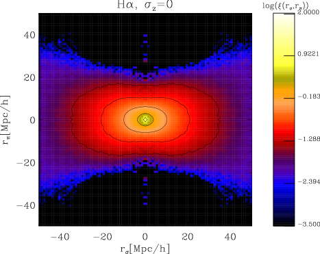
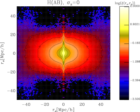
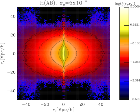
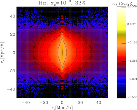
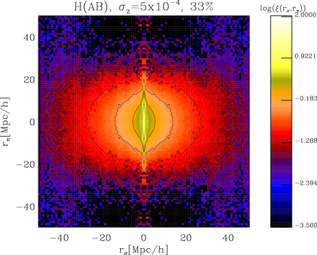
The impact of peculiar velocities on the clustering of galaxies is clearly seen in $\xi(r_{\sigma},r_{\pi})$. The top panels of Fig. 10 show the correlation function of $\mathrm{H}\alpha$ emitters selected to have $\mbox{${\rm log}(F_{H\alpha}\mbox{$[\mathrm{erg}\ \mathrm{s}^{-1}\ \mathrm{cm}^{-2}]$})$}>-16$ and $\mbox{$EW_{\mathrm{obs}}$}>100$Å (left) and H-band selected galaxies with $H_{\rm AB}<22$ (right). In the top and middle rows of Fig. 10, all galaxies are used down to the respective flux limits. To obtain clustering in redshift space, we use the distant observer approximation and give the galaxies a displacement along one of the cartesian axes, as determined by the component of the peculiar velocity along the same axis. Without peculiar velocities, contours of constant clustering amplitude in $\xi(r_{\sigma},r_{\pi})$would be circular. In redshift space, the clustering of H-band selected galaxies exhibits a clear signature on small scales of a contribution from high velocity dispersion systems – the so called “fingers of God”. This effect is less evident in the clustering of the $\mathrm{H}\alpha$ sample, as these galaxies avoid massive haloes, as shown in Fig. 8. On large scales, the contours of equal clustering are flattened due to coherent flows. Similar distortions have been measured in surveys such as the 2dFGRS (Hawkins et al. 2003) and the VLT-VIMOS deep survey (Guzzo et al. 2008).

In practice, the measured correlation functions will look somewhat different to the idealised results presented in the top row of Fig. 10. The redshift measurements will have errors, and the errors for slitless spectroscopy are expected to be bigger than those for slit-based spectroscopy (Euclid-NIS team, private communication). We model this by adding a Gaussian distributed velocity, $v_{r}$, to the peculiar velocities following $\delta z=(1+z)v_{r}/c$. The dispersion of the Gaussian is parametrized by $\sigma_{z}\equiv\langle\delta z^{2}\rangle^{1/2}/(1+z)$. We show the impact on the predicted clustering of adding illustrative redshift uncertainties to the position measurements in the middle and bottom panels of Fig. 10. For $\mathrm{H}\alpha$-emitters, we chose a fiducial error of $\sigma_{z}=10^{-3}$, based on simulations by the Euclid NIS team. The errors on the slit-based redshifts are expected to be at least a factor of 2 times smaller than the slitless errors, so we set $\sigma_{z}=5\times 10^{-4}$ for the $H_{\rm AB}$ selected sample. The impact of the redshift errors is most prominent in the case of the $\mathrm{H}\alpha$ sample, where the contours of constant clustering become more elongated along the line-of-sight direction.

A measure of how well bulk flows can be constrained can be gained from the accuracy with which $\beta$ can be measured (Eq. (4)). We estimate $\beta$ by applying Eq. (3) to the ratio of the redshift space to real space correlation function on pair separations between $15-30h^{-1}$Mpc, which is close to the maximum pair separation out to which we can reliably measure clustering in the Millennium simulation volume. The introduction of redshift errors forces us to apply Eq. (3) to the measurements from the Millennium simulation on larger scales than in the absence of errors. We note that the ratio is noisy even for a box of the volume of the Millennium, and in practice we average the ratio by projecting down each of the cartesian axes. The real space correlation function is difficult to estimate on large scales, so a less direct approach would be applied to actual survey data (see e.g. Guzzo et al., 2008). Hence, our results will be on the optimistic side of what is likely to be attainable with future surveys. Ideally, we would like to apply Eq. (5) on as large a scale as possible. Kaiser’s derivation assumes that the perturbations are in the linear regime.

Table 2: Values of $\beta$ estimated from the ratio of the redshift space to real space correlation function for the fiducial samples at $z=1$. We consider $\mathrm{H}\alpha$ emitters with fluxes $\mbox{${\rm log}(F_{H\alpha}\mbox{$[\mathrm{erg}\ \mathrm{s}^{-1}\ \mathrm{cm}^{-2}]$})$}>[-15.4,-16]$ and H-band selected galaxies with $H_{AB}<[22,23]$. The table is divided into two parts. The first half assumes a redshift success rate of $100\%$ and the second a $33\%$ redshift success rate. Each segment is divided into two, showing the impact on $\beta$ of including the expected redshift uncertainties: $\sigma_{z}=10^{-3}$ for $\mathrm{H}\alpha$ emitters and $\sigma_{z}=5\times 10^{-4}$ for H-band selected samples. Column (1) shows $\beta_{\rm lin}$, the exact theoretical value of $\beta$ obtained when using Eq. (4). Column (2) shows $\beta_{m}$, the value of $\beta$ measured in the simulation including the 1 $\sigma$ error. Column (3) shows the fractional error on $\beta_{m}$ using the Millennium volume. Column (4) shows the fractional error on $\beta_{m}$ obtained when using mock catalogues from the BASICC simulation.

	(1)	(2)	(3)	(4)
	$\beta_{lin}$	$\beta_{m}$	$(\delta\beta_{m}/\beta_{lin})$	$(\delta\beta_{m}/\beta_{lin})$
			Millennium	BASICC
Sampling rate = 100%
$\log(F(H\alpha))>-15.4$, $\sigma_{z}=0$	$0.761$	$0.684\pm 0.153$	$0.201$	$0.125$
$\log(F(H\alpha))>-16.0$, $\sigma_{z}=0$	$0.821$	$0.766\pm 0.027$	$0.034$	$0.021$
$H(AB)<22$, $\sigma_{z}=0$	$0.521$	$0.491\pm 0.026$	$0.051$	$0.019$
$H(AB)<23$, $\sigma_{z}=0$	$0.565$	$0.536\pm 0.013$	$0.023$	$0.013$
$\log(F(H\alpha))>-15.4$, $\sigma_{z}=10^{-3}$	$0.761$	$0.768\pm 0.170$	$0.224$	$0.122$
$\log(F(H\alpha))>-16.0$, $\sigma_{z}=10^{-3}$	$0.821$	$0.825\pm 0.058$	$0.071$	$0.081$
$H(AB)<22$, $\sigma_{z}=5\times 10^{-4}$	$0.521$	$0.527\pm 0.029$	$0.057$	$0.012$
$H(AB)<23$, $\sigma_{z}=5\times 10^{-4}$	$0.565$	$0.569\pm 0.012$	$0.022$	$0.008$
Sampling rate = 33%
$\log(F(H\alpha))>-15.4$, $\sigma_{z}=0$	$0.634$	$0.123\pm 0.447$	$0.704$	$0.449$
$\log(F(H\alpha))>-16.0$, $\sigma_{z}=0$	$0.807$	$0.680\pm 0.104$	$0.129$	$0.033$
$H(AB)<22$, $\sigma_{z}=0$	$0.516$	$0.482\pm 0.049$	$0.095$	$0.036$
$H(AB)<23$, $\sigma_{z}=0$	$0.568$	$0.569\pm 0.029$	$0.051$	$0.018$
$\log(F(H\alpha))>-15.4$, $\sigma_{z}=10^{-3}$	$0.634$	$0.300\pm 0.216$	$0.341$	$0.341$
$\log(F(H\alpha))>-16.0$, $\sigma_{z}=10^{-3}$	$0.807$	$0.749\pm 0.118$	$0.146$	$0.078$
$H(AB)<22$, $\sigma_{z}=5\times 10^{-4}$	$0.516$	$0.494\pm 0.061$	$0.118$	$0.023$
$H(AB)<23$, $\sigma_{z}=5\times 10^{-4}$	$0.568$	$0.603\pm 0.028$	$0.050$	$0.012$

We solve the integral for the growth rate $D$ in Eq. (4) (see Lahav et al., 1991) and use this exact result with the value of the bias $b$ measured for each galaxy sample to get the theoretical value $\beta_{\rm lin}$. Table 2 shows the comparison between $\beta_{m}$, the measured value of $\beta$ in the simulation, and target theoretical value $\beta_{\rm lin}$. Two different selection cuts are chosen for both $\mathrm{H}\alpha$ and H-band samples to cover a range of survey configurations: $\mbox{${\rm log}(F_{H\alpha}\mbox{$[\mathrm{erg}\ \mathrm{s}^{-1}\ \mathrm{cm}^{-2}]$})$}>[-15.4,-16.0]$ for $\mathrm{H}\alpha$ samples and $H_{AB}<[22,23]$ for the magnitude limited samples. All the mock catalogues studied return a value for $\beta_{m}$ which is systematically below the expected value, $\beta_{\rm lin}$.

Figure 11: The effective bias (top panel), number density of galaxies (middle panel) and the product $\bar{n}P$ (bottom panel) as functions of redshift, where $P$ is measured at wavenumber $k=0.2$ Mpc/h. The solid lines show the predictions for the Bau05(r) model and the Bow06(r) model is shown using dashed lines. The two columns show different $\mathrm{H}\alpha$ and H-band selections: In the first column the $\mathrm{H}\alpha$ sample is defined by a limiting flux of $\mbox{${\rm log}(F_{H\alpha}\mbox{$[\mathrm{erg}\ \mathrm{s}^{-1}\ \mathrm{cm}^{-2}]$})$}>-16$ and $\mbox{$EW_{\mathrm{obs}}$}>100$Å (red curves). The magnitude limited sample has $H_{AB}<22$ (blue curves). In the second column the $\mathrm{H}\alpha$ sample has $\mbox{${\rm log}(F_{H\alpha}\mbox{$[\mathrm{erg}\ \mathrm{s}^{-1}\ \mathrm{cm}^{-2}]$})$}>-15.4$ and $\mbox{$EW_{\mathrm{obs}}$}>100$Å, and the H-band sample has $H(AB)<23$. In all panels the redshift success rate considered is 100%.

When redshift errors are omitted and a 100% redshift success rate is used, both selection methods seem to reproduce the expected value of $\beta_{\rm lin}$ to within better than $\sim 10\%$. When redshift errors are included, the spatial distribution along the line of sight appears more elongated than it would be if the true galaxy positions could be used. This leads to an increase in the small scale damping of the clustering. However, at the same time contours of constant clustering amplitude are pushed out to larger pair separations in the radial direction. This results in an increase in the ratio of redshift space to real space clustering and an increase in the recovered value of $\beta$. When including the likely redshift errors, the values of $\beta_{m}$ found are slightly higher than those without redshift errors. This small boost in the value of $\beta_{m}$ is greatest in the $\mathrm{H}\alpha$ sample, because of the larger redshift errors than in the H-band sample.

We have also tested the impact of applying different redshift success rates on the determination of $\beta_{m}$. The lower part of Table 2 shows the impact of a $33\%$ redshift success rate. For $\mbox{${\rm log}(F_{H\alpha}\mbox{$[\mathrm{erg}\ \mathrm{s}^{-1}\ \mathrm{cm}^{-2}]$})$}>-15.4$, our results for $\beta_{m}$ shows that it is unlikely to get a robust estimate of $\beta$ at this flux limit, because the smaller number density makes the correlation functions very noisy, thus making $\beta_{m}$ impossible to be measured correctly. In contrast, the impact of a $33\%$ of success rate in the $\mbox{${\rm log}(F_{H\alpha}\mbox{$[\mathrm{erg}\ \mathrm{s}^{-1}\ \mathrm{cm}^{-2}]$})$}>-16$ sample is negligible. The $\beta_{m}$ values calculated using the H-band catalogues are also mostly unaffected. When redshift uncertainties are considered, as before, the $\beta_{m}$ values are closer to the theoretical $\beta_{lin}$. Hence redshift uncertainties will contribute to the uncertainty on $\beta_{m}$, but they still permit an accurate determination of $\beta$, provided they do not exceed $\sigma_{z}=10^{-3}$.

The noisy correlation functions for the configurations with $\mbox{${\rm log}(F_{H\alpha}\mbox{$[\mathrm{erg}\ \mathrm{s}^{-1}\ \mathrm{cm}^{-2}]$})$}>-15.4$ and sampling rate of 33% produce measurements of $\beta_{m}$ with large errors. The mock catalogues used so far in this section were created from the Millennium simulation, which has $V_{\rm Mill}=500^{3}{\rm[Mpc/h]^{3}}$. This volume is almost three orders of magnitude smaller than the volume expected in a large redshift survey from a space mission like Euclid(see next section). In order to test the impact of using this limited volume when measuring $\beta_{m}$ and its error, we plant the Bow06(r) model into a larger volume using the BASICC N-body simulation (Angulo et al., 2008a), which has a volume almost 20 times larger than the Millennium run ($V_{\rm BASICC}=1340^{3}{\rm[Mpc/h]^{3}}$). The errors on $\beta_{m}$ shown in Table  2 are expected, to first order, to scale with the error on the power spectrum (see Eq. (6) below). If we compare two galaxy samples with the same number density but in different volumes, then the error on $\beta_{m}$ should scale as $\delta\beta\propto 1/\sqrt{V}$, where $V$ is the volume of the sample.

The only drawback of using the BASICC simulation is that the mass resolution is worse than in the Millennium simulation. Haloes with mass greater than $5.5\times 10^{11}M_{\odot}/h$ can be resolved in the BASICC simulation. The galaxy samples studied here are hosted by haloes with masses greater than $\sim 8\times 10^{10}M_{\odot}/h$, so if we only plant galaxies into haloes resolved in the BASICC run then we would miss a substantial fraction of the galaxies. To avoid this incompleteness, those galaxies which should be hosted by haloes below the mass resolution limit are planted on randomly selected ungrouped particles, i.e. dark matter particles which do not belong to any halo. This scheme is approximate and works best if the unresolved haloes have a bias close to unity, i.e. where the bias is not a strong function of mass. This is almost the case in the application of this method to the BASICC run, so the clustering amplitude appears slightly boosted for all the configurations studied here. However, since we only want to study the variation in the error on $\beta_{m}$ when using a larger volume, we apply the same method described above to measure $\beta_{m}$ in the galaxy samples planted in the BASICC run.

As shown in the fourth column of Table  2, we find that for all the $\mathrm{H}\alpha$ configurations here studied the error on $\beta_{m}$ obtained when using the BASICC simulation is a factor 1-6 smaller than that found with the Millennium samples. The H-band samples, on the other hand, have errors roughly $\sim 4$ times smaller in the BASICC volume compared to the Millennium volume, which is what we expect if we assume that the error on $\beta_{m}$ scales with $1/\sqrt{V}$.

The Euclid survey will cover a geometrical volume of $\sim 90{\rm[Gpc/h]^{3}}$ with an effective volume of around half of this (see next section). We expect that Euclid should meausre $\beta_{m}$ with an accuracy around 5 times smaller than that estimated for the galaxy samples planted into the BASICC simulation.

4.4 Effective survey volume

Ongoing and future surveys aim to measure the baryonic acoustic oscillation (BAO) signal in the power spectrum of galaxies. The primary consideration for an accurate power spectrum measurement is to maximize the survey volume in order to maximize the number of independent $k$-modes. However, because the power spectrum is measured using a finite number of galaxies there is an associated discreteness noise. The number density of galaxies in a flux limited sample drops rapidly with increasing redshift, which means that discreteness noise also increases. When the discreteness noise becomes comparable to the power spectrum amplitude, it is difficult to measure the clustering signal. This trend is encapsulated in the expression for the fractional error on the power spectrum derived by Feldman, Kaiser & Peacock (1994):

$$\frac{\sigma}{P} \approx \frac{2\pi}{\sqrt{Vk^{2}\Delta k}}\left(1+\frac{1}{\bar{n}P}\right),$$ (6)

$$\approx \frac{2\pi}{\sqrt{V_{\rm eff}(k)k^{2}\Delta k}},$$ (7)

where $\sigma$ is the error on the power spectrum $P$, $V$ is the geometrical survey volume and $\bar{n}$ is the number density of galaxies. When the contrast of the power spectrum is high, i.e. $\bar{n}P\gg 1$, then the fractional error scales as the inverse square root of the survey volume. However, in the case that $\bar{n}P\leq 1$, the gain in accuracy from increasing the survey volume is less than the inverse square root of the increased volume. The amplitude of the power spectrum compared to the discreteness noise of the galaxies used to trace the density field is therefore a key consideration when assessing the effectiveness of different tracers of the large scale structure of the Universe.

Figure 12: The effective volume of $\mathrm{H}\alpha$- and H-band selected samples. The left-hand panels show results for Bau05(r) model and the right-hand panels show the Bow06(r) model; in the latter case, the effective volume for a randomly diluted sample of galaxies from the original Bow06  model is also shown. The upper row shows the effective volume divided by the geometrical volume in redshift shells of width $\Delta z=0.1$; the power spectrum at $k=0.2h{\rm Mpc}^{-1}$ is used to compute the effective volume (see text). The lower panels show the cumulative effective volume per steradian starting from $z=0.5$ and extending up to the redshift at which the curve is plotted. Red curves show the results for $\mathrm{H}\alpha$ selected galaxies with $\mbox{${\rm log}(F_{H\alpha}\mbox{$[\mathrm{erg}\ \mathrm{s}^{-1}\ \mathrm{cm}^{-2}]$})$}>-16$ and $\mbox{$EW_{\mathrm{obs}}$}>100$Å. The solid red line shows the result of applying a redshift success of $33\%$, whereas the red dashed line assumes a $100\%$ success rate. The blue lines show the results for an H-band magnitude selected survey with $H_{\rm AB}<22$. As before, the solid blue line shows the results for a sampling rate of $33\%$, and the dashed line assumes $100\%$ sampling. The green lines show the results using the Bow06  model diluted (Bow06(d)) to match the observed number counts; as before solid and dashed show 33% and 100% success rates, respectively. The black solid curves in the bottom panels show the total comoving volume covering the redshift range shown.

GALFORM gives us all the information required to estimate the effective volume of a survey with a given selection criteria (which defines the number density of galaxies, $\bar{n}(z)$, and the effective bias as a function of redshift). For simplicity, we use the linear theory power spectrum of dark matter, which is a reasonable approximation on the wavenumber scales studied here. The galaxy power spectrum is assumed to be given by $P_{\rm g}(k,z)=b(z)^{2}P_{\rm dm}(k,z)$, where $b(z)$ is the effective bias of the galaxy sample. We calculate the fraction of volume utilized in a given redshift interval following Tegmark (1997),

$$\mbox{$V_{\rm eff}$}(k,z)=\int_{z_{\rm min}}^{z_{\rm max}}\left[\frac{\bar{n}(z)P_{\rm g}(k,z)}{1+\bar{n}(z)P_{\rm g}(k,z)}\right]^{2}\frac{{\rm d}V}{{\rm d}z}{\rm d}z,$$ (8)

where all quantities are expressed in comoving coordinates. We calculate $\mbox{$V_{\rm eff}$}/V$ for a range of possible survey configurations considering different limits in flux, $EW_{\mathrm{obs}}$, magnitude limit and redshift success rate (see Table 3). The redshift range is chosen to match that expected to be set by the near-infrared instrumentation to be used in future surveys.

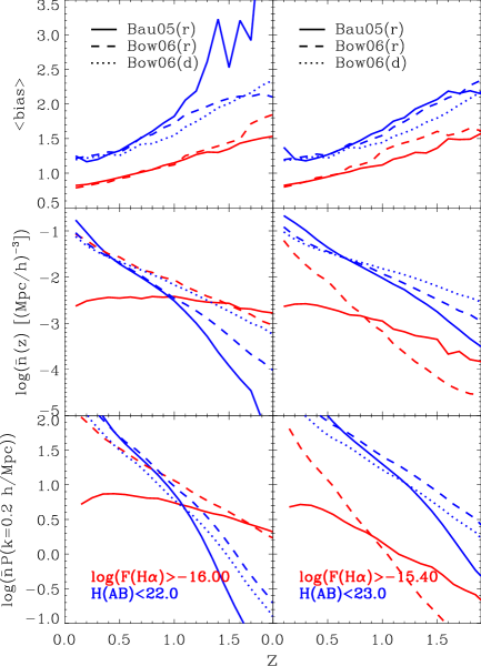
Fig. 11 shows the predictions from GALFORM which are required to compute the effective volume, for two illustrative $\mathrm{H}\alpha$ and H-band selected surveys, covering the current expected flux/magnitude limits of space missions. The bias predicted for H-band galaxies is at least $\sim 30\%$ higher than that for $\mathrm{H}\alpha$-emitters in both panels of Fig. 11. This reflects the different spatial distribution of these samples apparent in Fig. 8, in which is it clear that $\mathrm{H}\alpha$ emitters avoid cluster-mass dark matter haloes. The middle panel of Fig. 11 shows the galaxy number density as a function of redshift for these illustrative surveys. For the $\mathrm{H}\alpha$ selection, the models predict very different number densities at low redshifts, as shown also in Fig 7. For $z>1$ the Bow06(r) model predicts progressively more galaxies than the Bau05(r) model for the H-band selection. Overall, the number density of galaxies in the H-band sample at high redshift is much lower than that of $\mathrm{H}\alpha$ emitters. However, we remind the reader than these scaled models match the H-band counts but have a shallower redshift distribution than is suggested by the observations. The bottom panel of Fig. 11 shows the power spectrum times the shot noise, $\bar{n}P$, as a function of redshift. A survey which efficiently samples the available volume will have $\bar{n}P>1$. The slow decline of the number density of $\mathrm{H}\alpha$ galaxies with redshift in the Bau05(r) model is reflected in $\bar{n}P>1$ throughout the redshift range considered here, whereas in the Bow06(r) model, the $\mathrm{H}\alpha$ sample has a very steeply falling $\bar{n}P$ curve, with $\bar{n}P<1$ for $z>1.5$. The predictions of $\bar{n}P$ for the H-band are similar in both models, dropping below 1 at $z\sim 1.3-1.5$.

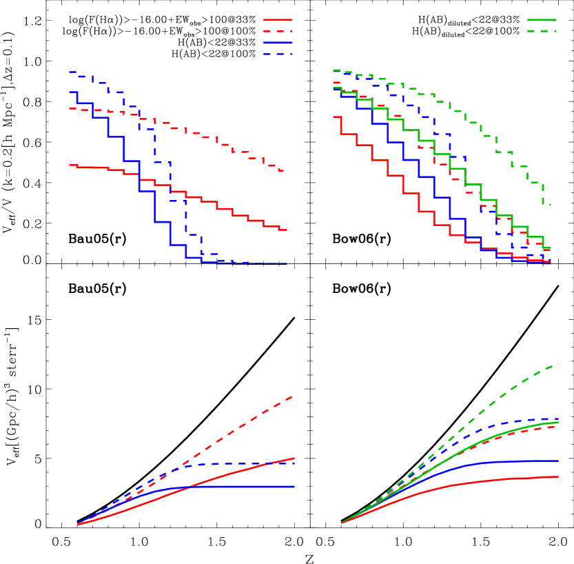
The predictions for the bias, number density and power spectrum of galaxies plotted in Fig. 11 are used in Eq. (8) to calculate the effective volume, which is shown in Fig. 12. The top panels show the differential $\mbox{$V_{\rm eff}$}/V$ calculated in shells of $\Delta z=0.1$ for redshifts spanning the range $z=[0.5,2]$. The bottom panels of Fig. 12 show the cumulative $V_{\rm eff}$ contained in the redshift range from $z=0.5$ up to $z=2$. We follow previous work and use the amplitude of the power spectrum at $k=0.2h{\rm Mpc^{-1}}$, which roughly corresponds to the centre of the wavenumber range over which the BAO signal is measured. We show the result for the fiducial survey selections with different redshift success rates, 100% and 33%. In addition, for the H-band selected survey, we also show the results obtained with the alternative approach discussed in the previous section, in which the galaxies in the Bow06  sample are diluted by a factor of 0.63.

Table 3: The effective volume of $\mathrm{H}\alpha$- and H-band selected surveys for different selection criteria. We evaluate a given survey configuration in terms of its effective volume in the redshift range $0<z<2$ (top) and $0.5<z<2$ (bottom), which is expressed as a fraction of the geometrical volume over the same redshift interval. The first column shows the galaxy selection method used, $\mathrm{H}\alpha$ for an $\mathrm{H}\alpha$ selected survey with a minimum flux limit and $EW_{\mathrm{obs}}$ cut or $H_{\rm AB}$ for an H-band magnitude limited survey. The second column shows the H-band magnitude limit chosen in a given configuration, where applicable. The third column shows the minimum $\mathrm{H}\alpha$ flux chosen, again where applicable, and the fourth column the minimum $EW_{\mathrm{obs}}$cut applied. The fifth column shows the redshift success rate assumed. Columns 6, 7 and 8 show the fractional effective volume obtained for a given configuration in the Bau05 , Bow06  and the diluted version of the Bow06   model respectively. Finally, columns 9, 10 and 11 show our estimate of the corresponding percentage error on the determination of $w$, the dark energy equation of state parameter, for the Bau05 , Bow06  and diluted Bow06  models, respectively.

Selection	$H_{\rm AB}$	${\rm log(F_{H\alpha})}$	$EW_{\mathrm{obs}}$	Sampling	$\mbox{$V_{\rm eff}$}/V$	$\mbox{$V_{\rm eff}$}/V$	$\mbox{$V_{\rm eff}$}/V$	$\Delta w(\%)$	$\Delta w(\%)$	$\Delta w(\%)$
	(mags)	${\rm(ergs^{-1}cm^{-2})}$	(Å)	rate	Bau05(r)	Bow06(r)	$\texttt{Bow06}\,_{\rm dil}$	Bau05(r)	Bow06(r)	$\texttt{Bow06}\,_{\rm dil}$
$0<z<2$
$\mathrm{H}\alpha$	-	-15.40	100	0.33	0.08	0.09	0.00	1.2	1.1	0.0
$\mathrm{H}\alpha$	-	-15.40	100	1.00	0.24	0.18	0.00	0.7	0.8	0.0
$\mathrm{H}\alpha$	-	-15.40	0	1.00	0.24	0.18	0.00	0.7	0.8	0.0
$\mathrm{H}\alpha$	-	-15.70	100	0.33	0.19	0.20	0.00	0.8	0.7	0.0
$\mathrm{H}\alpha$	-	-15.70	100	1.00	0.44	0.39	0.00	0.5	0.5	0.0
$\mathrm{H}\alpha$	-	-15.70	0	1.00	0.45	0.39	0.00	0.5	0.5	0.0
$\mathrm{H}\alpha$	-	-16.00	100	0.33	0.34	0.41	0.00	0.6	0.5	0.0
$\mathrm{H}\alpha$	-	-16.00	100	1.00	0.63	0.67	0.00	0.4	0.4	0.0
$\mathrm{H}\alpha$	-	-16.00	0	1.00	0.64	0.67	0.00	0.4	0.4	0.0
H(AB)	21	-	-	0.33	0.13	0.13	0.22	1.0	0.9	0.7
H(AB)	21	-	-	1.00	0.18	0.21	0.38	0.8	0.7	0.5
H(AB)	22	-	-	0.33	0.23	0.30	0.45	0.7	0.6	0.5
H(AB)	22	-	-	1.00	0.33	0.47	0.68	0.6	0.5	0.4
H(AB)	23	-	-	0.33	0.41	0.57	0.68	0.5	0.4	0.4
H(AB)	23	-	-	1.00	0.59	0.78	0.86	0.4	0.3	0.3
	0.3
$0.5<z<2$
$\mathrm{H}\alpha$	-	-15.40	100	0.33	0.06	0.06	0.00	1.4	1.4	0.0
$\mathrm{H}\alpha$	-	-15.40	100	1.00	0.21	0.15	0.00	0.8	0.9	0.0
$\mathrm{H}\alpha$	-	-15.40	0	1.00	0.21	0.15	0.00	0.8	0.9	0.0
$\mathrm{H}\alpha$	-	-15.70	100	0.33	0.18	0.07	0.00	0.9	1.2	0.0
$\mathrm{H}\alpha$	-	-15.70	100	1.00	0.43	0.17	0.00	0.5	0.8	0.0
$\mathrm{H}\alpha$	-	-15.70	0	1.00	0.44	0.17	0.00	0.5	0.8	0.0
$\mathrm{H}\alpha$	-	-16.00	100	0.33	0.33	0.21	0.00	0.6	0.7	0.0
$\mathrm{H}\alpha$	-	-16.00	100	1.00	0.62	0.41	0.00	0.4	0.5	0.0
$\mathrm{H}\alpha$	-	-16.00	0	1.00	0.63	0.41	0.00	0.4	0.5	0.0
H(AB)	21	-	-	0.33	0.09	0.10	0.19	1.2	1.1	0.8
H(AB)	21	-	-	1.00	0.14	0.18	0.35	1.0	0.8	0.6
H(AB)	22	-	-	0.33	0.19	0.27	0.43	0.8	0.6	0.5
H(AB)	22	-	-	1.00	0.30	0.44	0.67	0.6	0.5	0.4
H(AB)	23	-	-	0.33	0.38	0.55	0.67	0.6	0.4	0.4
H(AB)	23	-	-	1.00	0.57	0.77	0.86	0.5	0.4	0.3

In general, the effective volume is close to the geometrical volume at low redshifts. This is because $\bar{n}P\gg 1$ at these redshifts. In the top panels of Fig. 12, where the differential $V_{\rm eff}$/V is plotted in shells of $\Delta z=0.1$, we see that shells at higher redshifts cover progressively smaller differential effective volumes. This is due to the overall decrease in the number density of galaxies beyond the peak in the redshift distribution (see Figs. 5, 7 and 11), which wins out over the more modest increase in the bias of the galaxies picked up with increasing redshift. The bottom panels of Fig. 12 show the same effect: at higher redshifts, the gain in effective volume is much smaller than the corresponding gain in the geometrical volume of the survey. We remind the reader that our calculation for the effective volume in the H-band using models with rescaled luminosities is likely to be an underestimate, as these models underpredict the observed high redshift tail of the redshift distribution. A better estimate is likely to be provided by the Bow06(d) model, in which the number of galaxies is adjusted by a making a random sampling, rather than by changing their luminosities. This case is shown by the green curves in Fig. 12.

The calculations presented in Fig. 12 are extended to a range of survey specifications in Table 3. This table shows calculations for two different redshift ranges: $0<z<2$ and $0.5<z<2$, and includes also the effect of applying different selection criteria and redshift success rates to $\mathrm{H}\alpha$ and H-band surveys. An $\mathrm{H}\alpha$ survey with a limiting flux of $\mbox{${\rm log}(F_{H\alpha}\mbox{$[\mathrm{erg}\ \mathrm{s}^{-1}\ \mathrm{cm}^{-2}]$})$}>-15.4$, an equivalent width $\mbox{$EW_{\mathrm{obs}}$}>100$Å and a sampling rate of $0.33$, similar to the baseline spectroscopic solution for Euclid, would have a very small $\mbox{$V_{\rm eff}$}/V\sim 0.04$ for the redshift interval $z=0.5-2$. In contrast, an H-band survey with $H_{\rm AB}<22$ and a sampling rate of $0.33$, an alternative spectroscopic solution for Euclid, has $\mbox{$V_{\rm eff}$}/V=0.19-0.27$ or even up to $\mbox{$V_{\rm eff}$}/V=0.43$ in the case of the diluted model. To reach a comparable effective volume, a $\mathrm{H}\alpha$ survey would need to reach a flux limit of at least $\mbox{${\rm log}(F_{H\alpha}\mbox{$[\mathrm{erg}\ \mathrm{s}^{-1}\ \mathrm{cm}^{-2}]$})$}>-16$ (at the same equivalent width cut and redshift success rate).

The calculation of the effective volume also allows us to make an indicative estimate of the accuracy with which the dark energy equation of state parameter, $w$, can be measured for a given survey configuration. Angulo et al. (2008a) used large volume N-body simulations combined with the GALFORM model to calculate the accuracy with which the equation of state parameter $w$ can be measured for different galaxy samples. They found a small difference ($\sim 10\%$) in the accuracy with which $w$ can be measured for a continuum magnitude limited sample and an emission line sample with the same number density of objects. Their results can be summarised by:

$$\Delta w(\%)=\frac{1.5\%}{\sqrt{\mbox{$V_{\rm eff}$}}},$$ (9)

where $V_{\rm eff}$is in units of $h^{-3}{\rm Gpc}^{3}$ and the constant of proportionality (in this case, 1.5) depends on which cosmological parameters are held fixed; in the present case models are considered in which the distance to the epoch of last scattering is fixed as the dark energy equation of state parameter varies. We obtain an estimate of the accuracy with which $w$ can be measured by inserting $V_{\rm eff}$into Eq. 9, which is shown in Table 3, for the Bau05 and Bow06  models.

5 Discussion and Conclusions

In this paper we have presented the first predictions for clustering measurements expected from future space-based surveys to be conducted with instrumentation sensitive in the near-infrared. We have used published galaxy formation models to predict the abundance and clustering of galaxies selected by either their $\mathrm{H}\alpha$ line emission or H-band continuum magnitude. The motivation for this exercise is to assess the relative performance of the spectroscopic solutions proposed for galaxy surveys in forthcoming space missions which have the primary aim of constraining the nature of dark energy.

The physical processes behind $\mathrm{H}\alpha$ and H-band emission are quite different. $\mathrm{H}\alpha$ emission is sensitive to the instantaneous star formation rate in a galaxy, as the line emission is driven by the number of Lyman continuum photons produced by massive young stars. Emission in the observer frame H-band typically probes the rest frame $R$-band for the proposed magnitude limits and is more sensitive to the stellar mass of the galaxy than to the instantaneous star formation rate.

The GALFORM code predicts the star formation histories of a wide population of galaxies, and so naturally predicts their star formation rates and stellar masses at the time of observation. Variation in galaxy properties is driven by the mass and formation history of the host dark matter halo. This is because the strength of a range of physical effects depend on halo properties such as the depth of the gravitational potential well or the gas cooling time. This point is most striking in our plot of the spatial distribution of $\mathrm{H}\alpha$ and H-band selected galaxies, Fig. 8. This figure shows remarkable differences in the way that these galaxies trace the underlying dark matter distribution. $\mathrm{H}\alpha$ emitters avoid the most massive dark matter haloes and trace out the filamentary structures surrounding them. The H-band emitters, on the other hand, are preferentially found in the most massive haloes. This difference in the spatial distribution of these tracers has important consequences for the redshift space distortion of clustering.

In this paper we have studied two published galaxy formation models, those of Baugh et al. (2005) and Bower et al. (2006). The models were originally tuned to reproduce a subset of observations of the local galaxy population and also enjoy notable successes at high redshift. We presented the first comparison of the model predictions for the properties of $\mathrm{H}\alpha$ emitters, extending the work of Le Delliou et al. (2005, 2006) and Orsi et al. (2008) who looked at the nature of Lyman-alpha emitters in the models. Observations of $\mathrm{H}\alpha$ emitters are still in their infancy and the datasets are small. The model predicitions bracket the current observational estimates of the luminosity function of emitters and are in reasonable agreement with the distribution of equivalent widths.

The next step towards making predicitions of the effectiveness of future redshift surveys is to construct mock catalogues from the galaxy formation models (see Baugh, 2008). Using the currently available data, we used various approaches to fine tune the models to reproduce the observations as closely as possible. The main technique was to rescale the line and continuum luminosities of model galaxies; another approach was to randomly dilute or sample galaxies from the catalogue. This allowed us to better match the number of observed galaxies. The resulting mocks gave reasonable matches to the available clustering data around $z\sim 2$. Our goal in this paper was to make faithful mock catalogues. The nature of $\mathrm{H}\alpha$ emitters in hierarchical models will be pursued in a future paper.

The ability of future surveys to measure the large scale structure of the Universe can be quantified in terms of their effective volumes. The effective volume takes into account the effect of the discreteness of sources on the measurment of galaxy clustering. If the discreteness noise is comparable to the clustering signal, it becomes hard to extract any useful clustering information. Once this point is reached, although the available geometrical volume is increased by going deeper in redshift, in practice there is little point as no further statistical power is being added to the clustering measurments. The error on a power spectrum or correlation function measurement scales as the inverse square root of the effective volume. In the case of flux-limited samples, the number density of sources falls rapidly with increasing redshift beyond the median redshift. Even though the effective bias of these galaxies tends to increase with redshift, it does not do so at a rate sufficient to offset the decline in the number density. The GALFORM model naturally predicts the abundance and clustering strength of galaxies needed to compute the effective volume of a galaxy survey.

The differences in the expected performance of $\mathrm{H}\alpha$ and H-band selected galaxies when measuring the power spectrum is related to the different nature of the galaxies selected by these two methods. $\mathrm{H}\alpha$ emitters are active star forming galaxies, which makes them have smaller bias compared to H-band selected galaxies. Their redshift distribution is also very sensitive to the details of the physics of star formation: The effect of a top-heavy IMF in bursts in the Bau05  model boosts the number density of bright emitters, making the redshift distrubtion of $\mathrm{H}\alpha$ emitters very flat and slowly decreasing towards high redshifts, in contrast to the predictions of the Bow06  model, where a sharp peak at $z\sim 0.5$ and a rapid decrease for higher redshifts is found. H-band galaxies are less sensitive to this effect, and the redshift distributions are similar in both models. This is why the balance between the power spectrum amplitude (given by the effective bias) and the number density is translated in two different effective volumes for $\mathrm{H}\alpha$ and H-band selected galaxies.

Although there are differences in detail between the model predictions, they give similar bottom lines for the effective volumes of the survey configurations of each galaxy selection. Comparing the spectroscopic solutions in Table 3, a slit based survey down to $H_{\rm AB}=22$ would sample 4-10 times the effective volume which could be reached by a slitless survey to $\mbox{${\rm log}(F_{H\alpha}\mbox{$[\mathrm{erg}\ \mathrm{s}^{-1}\ \mathrm{cm}^{-2}]$})$}=-15.4$, taking into account the likely redshift success rate. To match the performance of the H-band survey, an $\mathrm{H}\alpha$ survey would need to go much deeper in flux, down to $\mbox{${\rm log}(F_{H\alpha}\mbox{$[\mathrm{erg}\ \mathrm{s}^{-1}\ \mathrm{cm}^{-2}]$})$}=-16$.

We have also looked at the accuracy with which $\mathrm{H}\alpha$ emitters and H-band selected galaxies will be able to measure the bulk motions of galaxies and hence the rate at which fluctuations are growing, another key test of gravity and the nature of dark energy. All of the samples we considered showed a small systematic difference between the measured growth rate and the theoretical expectation, at about the $1\sigma$ level. The error on the growth rate from an $\mathrm{H}\alpha$ survey with $\mbox{${\rm log}(F_{H\alpha}\mbox{$[\mathrm{erg}\ \mathrm{s}^{-1}\ \mathrm{cm}^{-2}]$})$}>-15.4$ was found to be about three times larger than that for a sample with $H_{AB}<22$.

References

- Albrecht et al. (2006) Albrecht A., Bernstein G., Cahn R., et al., 2006, astro, arXiv:astro-ph/0609591
- Almeida, Baugh & Lacey (2007) Almeida C., Baugh C.M., Lacey C.G., 2007, MNRAS, 376, 1711
- Almeida et al. (2008) Almeida C., Baugh C.M., Wake D.A., Lacey C.G., Benson A.J., Bower R.G., Pimbblet K., 2008, MNRAS, 386, 2145
- Angulo et al. (2008a) Angulo R. E., Baugh C. M., Frenk C. S., Lacey C. G., 2008a, MNRAS, 383, 755
- Angulo et al. (2008b) Angulo R. E., Baugh C. M., Lacey C. G., 2008b, MNRAS, 387, 921
- Baugh (2006) Baugh, C.M., 2006, Rep. Prog. Phys., 69, 3101
- Baugh (2008) Baugh, C.M., 2008, Phil Trans A, 366, 4381
- Baugh et al. (1999) Baugh C. M., Benson A. J., Cole S., Frenk C. S., Lacey C. G., 1999, MNRAS, 305, L21
- Baugh et al. (2005) Baugh C.M., Lacey C.G., Frenk C.S., Granato G.L., Silva L., Bressan A., Benson A.J., Cole S., 2005, MNRAS, 356, 1191
- Benson et al. (2003) Benson A. J., Bower R. G., Frenk C. S., Lacey C. G., Baugh C. M., Cole S., 2003, ApJ, 599, 38
- Blake et al. (2009) Blake C., Jurek R. J., Brough S., et al., 2009, MNRAS, 395, 240
- Bower et al. (2006) Bower R. G., Benson A. J., Malbon R., Helly J. C., Frenk C. S., Baugh C. M., Cole S., Lacey C. G., 2006, MNRAS, 370, 645
- Cannon et al. (2006) Cannon R., Drinkwater M., Edge A., et al., 2006, MNRAS, 372, 425
- Cirasuolo et al. (2008) Cirasuolo M., McLure R.J., Dunlop J.S., Almaini O., Foucaud S., Simpson C., 2008, MNRAS, submitted. arXiv:0804.3471
- Cole et al. (1994) Cole S., Fisher K. B., Weinberg D. H., 1994, MNRAS, 267, 785
- Colless et al. (2003) Colless M., Peterson B. A., Jackson C., et al., 2003, astro, arXiv:astro-ph/0306581
- Chen et al. (2002) Chen H.-W., McCarthy P. J., Marzke R. O., et al., 2002, ApJ, 570, 54
- Cimatti et al. (2009) Cimatti A., et al., 2009, ExA, 23, 39
- Cole & Kaiser (1989) Cole S., Kaiser N., 1989, MNRAS, 237, 1127
- Cole et al. (2000) Cole S., Lacey C.G., Baugh C.M., Frenk C.S., 2000, MNRAS, 319, 168
- Croton et al. (2005) Croton D.J., Springel V., White S.D.M., De Lucia G., Frenk C.S., Gao L., Jenkins A., Kauffmann G., Navarro J.F., Yoshida N., 2006, MNRAS, 365, 11
- Feldman, Kaiser & Peacock (1994) Feldman H. A., Kaiser N., Peacock J.A., 1994, ApJ, 426, 23
- Firth et al. (2002) Firth A. E., Somerville R. S., McMahon R. G., et al., 2002, MNRAS, 332, 617
- Frith et al. (2006) Frith W. J., Metcalfe N., Shanks T., 2006, MNRAS, 371, 1601
- Fujita et al. (2003) Fujita S. S., Ajiki M., Shioya Y., et al., 2003, ApJ, 586, L115
- Gao, Springel & White (2005) Gao L., Springel V., White S. D. M., 2005, MNRAS, 363, L66
- Gao & White (2007) Gao L., White S.D.M., 2007, MNRAS, 377, L5
- Gawiser et al. (2007) Gawiser E., et al., 2007, ApJ, 671, 278
- Geach et al. (2008) Geach J. E., Smail I., Best P. N., Kurk J., Casali M., Ivison R. J., Coppin K., 2008, MNRAS, 388, 1473
- Geach et al. (2009) Geach J. E. et al. 2009, submitted.
- Gonzalez et al. (2009) Gonzalez J. E., Lacey C. G., Baugh C. M., Frenk C. S., Benson A. J., 2009, MNRAS, 397, 1254
- Gonzalez-Perez et al. (2009) Gonzalez-Perez V., Baugh C. M., Lacey C. G., Almeida C., 2009, MNRAS, 398, 497
- Groth & Peebles (1977) Groth E. J., Peebles P. J. E., 1977, ApJ, 217, 385
- Guzzo et al. (2008) Guzzo L., Pierleoni M., Meneux B., et al., 2008, Nature, 451, 541
- Hawkins et al. (2003) Hawkins E., Maddox S., Cole S., et al., 2003, MNRAS, 346, 78
- Helly et al. (2003) Helly J., Cole S., Frenk C.S., Baugh C.M., Benson A., Lacey C., 2003, MNRAS, 338, 903
- Hippelein et al. (2003) Hippelein H., Maier C., Meisenheimer K., et al., 2003, A&A, 402, 65
- Hopkins et al. (2000) Hopkins A. M., Connolly A. J., Szalay A. S., 2000, AJ, 120, 2843
- Jones & Bland-Hawthorn (2001) Jones D. H., Bland-Hawthorn J., 2001, ApJ, 550, 593
- Kauffmann, White & Guiderdoni (1993) Kauffmann G., White S. D. M., Guiderdoni B., 1993, MNRAS, 264, 201
- Kaiser (1984) Kaiser N., 1984, ApJ, 284, L9
- Kaiser (1987) Kaiser N., 1987, MNRAS, 227, 1
- Kennicutt (1983) Kennicutt R. C., Jr., 1983, ApJ, 272, 54
- Kim et al. (2009) Kim H. S., Baugh C. M., Cole S., Frenk C. S., Benson A. J., 2009, MNRAS, in press, arXiv:0905.4723
- Lacey et al. (2008) Lacey C.G., Baugh C.M., Frenk C.S., Silva L., Granato G.L., Bressan A., 2008, MNRAS, 385, 1155
- Lahav et al. (1991) Lahav O., Lilje P. B., Primack J. R., Rees M. J., 1991, MNRAS, 251, 128
- Le Delliou et al. (2005) Le Delliou, M., Lacey, C., Baugh, C.M., Guiderdoni, B., Bacon, R., Courtois, H., Sousbie, T., Morris, S.L., 2005, MNRAS, 357, L11
- Le Delliou et al. (2006) Le Delliou, M., Lacey, C. G., Baugh, C. M., Morris, S. L., 2006, MNRAS, 365, 712
- Lue, Scoccimarro & Starkman (2004) Lue A., Scoccimarro R., Starkman G., 2004, PhRvD, 69, 044005
- Martini (2001) Martini P., 2001, AJ, 121, 598
- McCarthy et al. (1999) McCarthy P., Marzke R., Chen H. W., et al., 1999, AAS, 31, 1459
- Metcalfe et al. (2006) Metcalfe N., Shanks T., Weilbacher P. M., McCracken H. J., Fong R., Thompson D., 2006, MNRAS, 370, 1257
- Mo & White (1996) Mo H.J., White S.D.M., 1996, MNRAS, 282, 347
- Morioka et al. (2008) Morioka T., Nakajima A., Taniguchi Y., Shioya Y., Murayama T., Sasaki S. S., 2008, PASJ, 60, 1219
- Moy (2003) Moy E., Barmby P., Rigopoulou D., Huang J.-S., Willner S. P., Fazio G. G., 2003, A&A, 403, 493
- Nakajima et al. (2008) Nakajima A., Shioya Y., Nagao T., Saito T., Murayama T., Sasaki S. S., Yokouchi A., Taniguchi Y., 2008, PASJ, 60, 1249
- Orsi et al. (2008) Orsi A., Lacey C.G., Baugh C.M., Infante L., 2008, MNRAS, 391, 1589
- Osterbrock (1989) Osterbrock D.E., 1989, Astrophysics of gaseous nebulae and active galactic nuclei, University of Minnesota, University Science Books.
- Pascual et al. (2001) Pascual S., Gallego J., Aragón-Salamanca A., Zamorano J., 2001, A&A, 379, 798
- Peacock et al. (2006) Peacock J. A., Schneider P., Efstathiou G., Ellis J. R., Leibundgut B., Lilly S. J., Mellier Y., 2006, ewg3.rept, astro-ph:0610906
- Peebles (1980) Peebles P. J. E., 1980, The Large-Scale Structure of the Universe (Princeton: Princeton Univ. Press)
- Retzlaff et al. (2009) Retzlaff J., Rosatti P., Dickinson M., Vandame B., Rite C., Noino M., Cesarsky C., and the GOODS Team., submitted
- Ross et al. (2007) Ross N. P., Shanks T., Cruz da Ângela J., 2007, ASPC, 379, 68
- Scoccimarro (2004) Scoccimarro R., 2004, PhRvD, 70, 083007
- Sheth, Mo & Tormen (2001) Sheth R. K., Mo H. J., Tormen G., 2001, MNRAS, 323, 1
- Shim et al. (2009) Shim H., Colbert J., Teplitz H., Henry A., Malkan M., McCarthy P., Yan L., 2009, ApJ, 696, 785
- Shioya et al. (2008) Shioya Y., Taniguchi Y., Sasaki S. S., et al., 2008, ApJS, 175, 128
- Smith et al. (2003) Smith R. E., Peacock J. A., Jenkins A., et al., 2003, MNRAS, 341, 1311
- Sobral et al. (2009) Sobral D., Best P. N., Geach J. E., et al., 2009, arXiv, arXiv:0901.4114
- Springel et al. (2005) Springel V. et al., 2005, Nature, 435, 639
- Tegmark (1997) Tegmark M., 1997, Phys. Rev. Let., 79, 3806
- Teplitz et al. (1998) Teplitz H. I., Gardner J. P., Malumuth E. M., Heap S. R., 1998, ApJ, 507, L17
- Thompson et al. (1996) Thompson D., Mannucci F., Beckwith S. V. W., 1996, AJ, 112, 1794
- Thompson et al. (1999) Thompson R. I., Storrie-Lombardi L. J., Weymann R. J., Rieke M. J., Schneider G., Stobie E., Lytle D., 1999, AJ, 117, 17
- Tresse et al. (2002) Tresse L., Maddox S. J., Le Fèvre O., Cuby J.-G., 2002, MNRAS, 337, 369
- Villar et al. (2008) Villar V., Gallego J., Pérez-González P. G., Pascual S., Noeske K., Koo D. C., Barro G., Zamorano J., 2008, ApJ, 677, 169
- Wang (2008) Wang Y., 2008, JCAP, 05, 021
- Wang & Mukherjee (2007) Wang Y., Mukherjee P., 2007, PhRvD, 76, 103533
- Wechsler et al. (2006) Wechsler R. H., Zentner A. R., Bullock J. S., Kravtsov A. V., Allgood B., 2006, ApJ, 652, 71
- White & Rees (1978) White S. D. M., Rees M. J., 1978, MNRAS, 183, 341
- White (1991) White S. D. M., Frenk C. S., 1991, ApJ, 379, 52
- Yan et al. (1998) Yan L., McCarthy P. J., Storrie-Lombardi L. J., Weymann R. J., 1998, ApJ, 503, L19
- York et al. (2000) York D. G., Adelman J., Anderson J. E., Jr., et al., 2000, AJ, 120, 1579