A Brownian Dynamics Model of Kinesin in Three Dimensions Incorporating the Force-Extension Profile of the Coiled-Coil Cargo Tether

Abstract

The Kinesin family of motor proteins are involved in a variety of cellular processes that transport materials and generate force. With recent advances in experimental techniques, such as optical tweezers which can probe individual molecules, there has been an increasing interest in understanding the mechanisms by which motor proteins convert chemical energy into mechanical work. Here we present a mathematical model for the chemistry and three dimensional mechanics of the Kinesin motor protein which captures many of the force dependent features of the motor. For the elasticity of the tether that attaches cargo to the motor we develop a method for deriving the non-linear force-extension relationship from optical trap data. For the Kinesin heads, cargo, and microscope stage we formulate a three dimensional Brownian Dynamics model that takes into account excluded volume interactions. To efficiently compute statistics from the model an algorithm is proposed that uses a two step protocol that separates the simulation of the mechanical features of the model from the chemical kinetics of the model. Using this approach for a bead transported by the motor, the force dependent average velocity and randomness parameter are computed and compared with the experimental data.

The Kinesin family of motor proteins is involved in a variety of cellular processes including the transport of materials to the end of axons  (li1999, ), the controlled localization of organelles during cell development  (tuma1998, ), and the separation of chromosomes during mitosis  (sharp2000, ),  (karsenti2001, ). The vesicle and organelle transporting members of the Kinesin family interact with long microtubule filaments of the cytoskeleton. The filaments serve the dual purpose of giving a cell structural support and as a highway on which motor proteins transport materials between distant locations within the cell  (thecell, ).

The Kinesin motor protein consists of two homologous globular domains, referred to as “heads”  (vale1997, ). The heads are joined together by a long coiled-coil alpha-helix structure which extends to attach like a tether to cargo transported by the motor  (goldstein2001, ),  (kamal2002, ). The globular domains each have specialized regions that interact with tubulin dimers of the microtubules and a binding pocket for the nucleotide adenosine-tri-phosphate (ATP)  (woehlke1997, ).

The motor moves along the microtubule track by binding and unbinding its heads from interaction sites on the microtubule surface  (gilbert1995, ). The binding sites are spaced at approximately $8$-nm increments  (svoboda1993, ),  (hoenger2000, ),  (amos2000c, ). Microtubules have a polarity deriving from an asymmetry in their constituent monomer units  (nogales1999, ),  (downing1998, ). By convention the end toward which almost all of the Kinesin motors move is referred to as the plus end of the microtubule.

The motor is powered from energy released by breaking covalent bonds between the second and third phosphate group of (ATP) in a process known as hydrolysis. The detailed mechanism by which the energy released during hydrolysis is converted into mechanical work is presently unknown.

Individual Kinesin motor proteins have globular domains on the order of $10$-nm in diameter. On this small length scale thermal fluctuations arising from collisions of the protein with the constituent molecules of the surrounding solvent are significant and may play an important role in how the motor functions. The fluctuations affect both the internal structure of each of the heads as well as their diffusion, when unbound, relative to the microtubule. There have been many theoretical mechanisms proposed whereby the energy from hydrolysis and thermal fluctuations drive conformational changes, or more subtly, rectify fluctuations of protein structures to perform mechanical work  (howard2001, ),  (fox1998, ),  (julicher1997, ),  (bustamante2001, )  (knight1999, ),  (peskin1993, ).

Crystollographic structures for the Kinesin molecule have been solved in a few different conformations when bound to the products of the ATP hydrolysis cycle or analogue substrates  (kozielski1997, ),  (kull1996, ),  (mandelkow1999, ),  (rice1999, ),  (song2001, ),  (kikkawa2001, ),  (sindelar2002, ),  (yun2003, ),  (sack1997, )  (case2000b, ). The crystallographic structures and related mutagenesis studies yield many clues about which protein structures are important and how they might contribute to the operation of the motor protein.

From these structures a partial picture of how the motor operates is emerging. Connecting each head of Kinesin to the long coil-coiled structure is a sequence of approximately 15 amino acid residues referred to as the “neck-linker”. When the head is bound to different ATP hydrolysis products this structure undergoes conformational changes which are thought to perform the working “power stroke” of the motor which moves the lagging head closer toward the plus end of the microtubule  (rice1999, ),  (rice2003, ). A collection of loops and alpha helices have also been identified which interact with bound substrates. These structures are thought to be important in communicating the identity of the substrate to distant parts of the molecule. These “switch” structures affect such features of the motor as the binding affinity of a head for a microtubule and the conformation of the neck-linker  (kikkawa2001, ),  (schliwa2001, ),  (sablin2001, ).

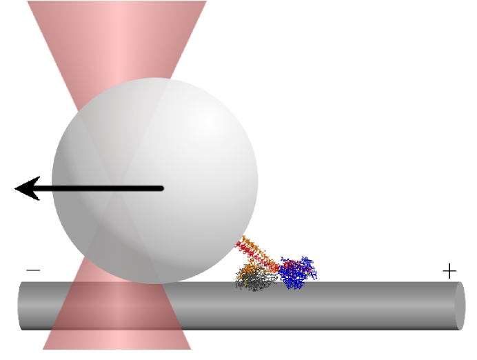
While crystallographic structures offer primarily a statistic geometric picture, optical trap experiments have been used to study the dynamics of individual motor proteins as they operate. To probe the motor, a latex bead hundreds of nanometers in diameter is attached to the protein through the long coiled-coil tether structure. A load force is applied to the cargo bead and the response of its transport by the motor is observed as the load force is varied. See figure 1. Since only the bead is observed, to obtain information about the motor, a separate experiment must be performed to obtain the elasticity of the tether which attaches the bead to the motor  (svobodaandblock1994, ).

Measurements from the optical trap experiments yield interesting information about how the motor functions. By performing repeated experiments it is possible to estimate force dependent statistics of individual Kinesin molecules such as the response of the motor velocity to a load force. The experimental data also place important constraints on candidate mechanisms for how the motor functions, such as the number of rate limiting “mechanochemical” events per 8-nm step along the microtubule. It has even been possible to deduce some information about the conformational changes that occur. Using high precision optical traps small systematic displacements of the bead have been estimated at high spatial and temporal resolution within the 8-nm steps of the motor  (nishiyama2001, ),  (coppin1996, ).

In modeling the optical trap experimental data a difficulty arises in modeling the motor protein. Attempting to model at a detailed level using methods such as molecular dynamics allows for simulation over only a short time relative to the time scale on which the motor operates and on which experimental measurements are made. The overall aim of this work is to derive a mechanical model of the motor at a coarse scale that allows for efficient computation of long time-scale observables.

Many models have been proposed for Kinesin  (mogilner2001, ),  (peskin1995, ),  (fisher2001, ),  (astumian1999, ),  (maes2003, ). In these papers Kinesin is often described by a single mechanical degree of freedom or reaction coordinate in which many details concerning the geometry and elasticity of the motor are neglected. In this work we propose a three dimensional mathematical model for the Kinesin motor protein taking into account basic structural features of the motor. Data from the optical trap experiments of  (svobodaandblock1994, ), in which the elasticity of the cargo tether of the motor is probed, are incorporated into the mechanics of the model. We show how a force-extension relationship for the tether can be derived from the published data. An algorithm is then proposed that exploits a separation of time scales in the model to efficiently compute statistics that can be compared with the optical trap experimental data.

Fig. 1: A Schematic Representation of the Optical Trap Experiment of Svoboda and Block 1994. A laser trap for the cargo bead is generated with a center of focus above the microtubule. The interaction of the laser light with the bead results in a restoring force that tends to pull the bead toward the focus of the laser. As the motor progresses along the microtubule toward the plus end, the bead is pulled successively further from the center of focus and an increasingly strong load force is exerted on the motor.

1 Model Description

Kinesin consists of two nearly homologous globular domains that form what are referred to as the “heads” of the motor protein. Each of the heads has a special binding site in which ATP hydrolysis occurs and each has a separate structure that interacts with microtubules. Extending from each of the heads is a long alpha helix that dimerizes the two heads by forming an intertwined coiled-coil structure. The coiled-coil structure also acts as a tether to attach cargo to the motor.

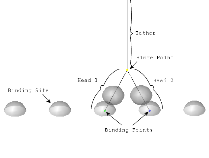
The detailed internal geometry of the two heads of Kinesin are neglected in the model and represented by two spherical excluded volumes. The microtubule binding sites of each head are modeled by control points extending from the surface of each excluded volume. The heads are connected to one another at a common point which we shall refer to as the “hinge point”. The coiled-coil tether is modeled as a non-linear spring with a force-extension relationship derived from experimental data. See section 2 for the details of this procedure. Figure 3 gives a schematic illustration of the model.

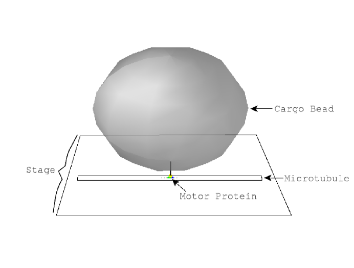
A bead is connected to the motor in optical trap experiments and is modeled by a large spherical excluded volume. The excluded volume interactions of the bead with the microscope stage, microtubule, and the motor are accounted for in the model. The interaction with the stage is enforced by a condition that the bead not move below a given planar surface. The detailed geometry of the stage mounted microtubule is neglected in the model since on the length scale of the bead it is expected that the microtubule appears as little more than a small “bump” on the stage surface only making a minor contribution to the bead diffusion dynamics. See figure 2 for a schematic of the model where the motor, microtubule, and cargo bead are drawn approximately to scale.

Microtubules serve as the track on which Kinesin moves. Typically 13 protofilaments join laterally to form a sheet that when rolled up forms the hollow cylindrical structure of the microtubule  (nogales1999, ). For dimeric Kinesins it has been found that the motor moves along the axis of a single protofilament of the microtubule. When the protofilaments are twisted so that they form a helical spiral that wraps around the microtubule it is found that dimeric Kinesin move in a similar helical spiral  (ray1993, ). This suggests that dimeric Kinesin binds to sites located in a regular pattern in the neighborhood of a protofilament. When considering single headed Kinesin molecules a more complex movement along microtubules has been observed  (berliner1995, ).

In the model we arrange the microtubule binding sites of the motor along a single protofilament spaced with $8$-nm increments. We model these sites by hemispherical regions of radius $2$-nm that interact with the binding control points of the Kinesin heads, see figure 3.

To model the state of the motor as it progresses through the coupled hydrolysis and mechanical stepping cycle, we make stochastic transitions determined by the chemical kinetics and mechanics of the motor protein. We postulate that each of the heads of Kinesin is in any of three broadly defined states. A head can be bound to a microtubule denoted (B), be freely diffusing with weak affinity for the binding sites (W), or be freely diffusing with strong affinity for the binding sides (S). The states of the motor as a whole consist of all pair combinations of theses affinities. We shall discuss the details of the admissible states and the specific mechanochemical cycle for our model below.

In summary, the mechanical model of the motor protein consists of two spherical excluded volumes connected at a common hinge point. The hinge point serves as the anchor for the tether that attaches cargo to the motor. The tether is modeled by a non-linear spring. The motor moves by successively binding and unbinding its heads from the track. When a head is unbound from the microtubule there is a joint diffusion of the cargo bead and the heads. When a head is bound to adjacent microtubule sites the the binding control points and the hinge point form an equilateral triangle with sides of length $8$-nm.

Fig. 2: Illustration of the Model Plotted Approximately to Scale

Fig. 3: Illustration of the Model with a Magnified View of the Motor

2 Reconstruction of the Tether Force-Extension Profile from Experimental Data

Extending from the motor domains of Kinesin is a long coiled-coil alpha helix structure which acts like a tether that attaches cargo transported by the motor protein. Since the forces acting on the cargo are transmitted to the motor by the coiled-coil structure the elasticity of the tether may play an important role how the motor operates when transporting cargo subject to a load force. In  (elston2000, ),  (elston2000b, ),  (chen2002, ) a linear force-extension relation for the tether was considered. It was shown that depending on the model of the motor protein different tether stiffnesses were optimal in the velocity attained by the motor. In this section we discuss a method by which a nonlinear force-extension relation for the coiled-coil structure can be derived from the data of the optical trap experiments of  (svobodaandblock1994, ).

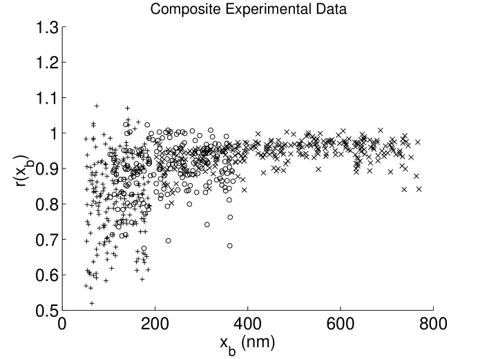
In the optical trap experiments of  (svobodaandblock1994, ) a bead is attached to an inactive Kinesin motor protein which is bound to a microtubule. The microtubule is mounted to a microscope stage which is moved at a fixed speed $V_{m}$. In the experimental data only two quantities are published. The first quantity is the velocity ratio $r=\frac{V_{b}}{V_{m}}$ where $V_{b}$ is the bead velocity and $V_{m}$ is the stage velocity. The second quantity is the component of the bead position in the direction of the microtubule $x_{b}=\mathbf{X}_{b}^{(1)}$, where in our notation $\mathbf{X}_{b}$ is the three dimensional position of the bead. The experimental data is published as the velocity ratio $r$ plotted as a function of the bead position $x_{b}$. figure 5.

To obtain the force-extension profile of the tether from the one dimensional observations of the experiment we must determine the extension of the tether for each observed bead position and the applied force that yields this extension. To obtain the correct relationship we must take into account the three dimensional geometry of the experiment.

In the experiment as the stage moves the tether pulls the bead from the center of the trap which then exerts an opposing optical restoring force. The bead also experiences random forces as a consequence of the thermal fluctuations of the surrounding solvent that cause it to diffuse in three dimensions subject to the deterministic forces of the system. As a consequence of the thermal fluctuations of the bead and the resolution of the experimental measurements, the data reflect averages of the quantities $r$ and $x_{b}$. It can be shown that the problem of precisely determining the restoring force of the tether and the extension of the tether from these observations is a mathematically ill-posed problem. However, if some operational assumptions are made an approximate force-extension profile can be reconstructed from the data.

2.1 Model of the Experiment and the Reconstruction Method

In the experiments of  (svobodaandblock1994, ) a $250$-nm latex bead was attached to the motor protein and the center of the optical trap was located $250$-nm above the microscope stage. This arrangement has the convenient feature of keeping the bead in a configuration which is in contact with the surface of the microscope stage. As a consequence some important simplifications can made in the derivation.

To avoid the difficulties of modeling the thermal fluctuations of the system we shall assume in our model that the stage velocity is slow relative to the time scale for the bead diffusion to reach its equilibrium distribution. Thus at each instant we shall make the operational assumption that on average all forces are balanced in the system and neglect further effects of the thermal fluctuations.

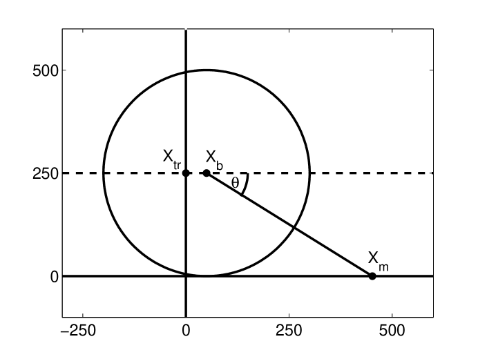
In the experiment the motor is bound in an inactive state at position $\mathbf{X}_{m}$ to a microtubule. The microtubule is mounted on the microscope stage. A cargo bead is attached through the coiled-coil tether structure to the motor. The bead is subject to the restoring force toward the center of the optical trap located at position $\mathbf{X}_{tr}$. As a consequence of the geometric setup of the experiment with the bead in contact with the stage, when the forces are balanced, the state of the system is described by the one dimensional components of the positions in the direction of the microtubule axis. These positions are denoted respectively by $x_{b}=\mathbf{X}_{b}^{(1)}$ for the bead, $x_{tr}=\mathbf{X}_{tr}^{(1)}$ for the trap, and $x_{m}=\mathbf{X}_{m}^{(1)}$ for the motor. An illustration of the geometry of the experiment is given in figure 4.

In the experiment, calibration measurements were made to obtain the restoring force of the optical trap. This was found to be approximated well by a linear spring. In our model we shall treat the force acting on the bead in the direction of the microtubule arising from the optical trap by the linear spring $K_{tr}(x_{b}-x_{tr})$, in which the spring stiffness $K_{tr}$ has been estimated for each laser power by calibration measurements. The assumption of balance of forces for each configuration $x_{b}$ of the bead and motor $x_{m}$ requires that the tether force $F_{tether}$ balance the force of the optical trap in the direction of the microtubule axis. This requires that the tether force satisfy

$$F_{tether}\cdot\cos(\theta)=K_{tr}(x_{b}-x_{tr})$$ (1)

where $\theta$ is the angle the tether makes when binding the cargo bead as illustrated in figure 4.

From this model we find that in order to obtain the tether force $F_{tether}$ and the extension of the tether $L$ we must determine the angle $\theta$ from the experimental data. This is equivalent to knowing the value of $x_{m}$ for each observation $x_{b}$. We can obtain the motor position $x_{m}$ from the observations of $x_{b}$ and $r(x_{b})$ using the following approximations.

$$r=\frac{V_{b}}{V_{m}}\approx\frac{\frac{\Delta{x_{b}}}{\Delta{t}}}{\frac{\Delta{x_{m}}}{\Delta{t}}}\approx\frac{\Delta{x_{b}}}{\Delta{x_{m}}}\approx\frac{dx_{b}}{dx_{m}}$$ (2)

Thus we can relate $x_{m}$ to the observed quantities $x_{b}$ and $r(x_{b})$ by using the experimental data to numerically evaluate the following integral.

$$x_{m}(x_{b})-x_{m}^{0} = \int_{x_{b}^{0}}^{x_{b}}\frac{\partial x_{m}}{\partial{x_{b}^{\prime}}}dx_{b}^{\prime}$$

$$= \int_{x_{b}^{0}}^{x_{b}}1/r(x_{b}^{\prime})dx_{b}^{\prime}$$

We remark that this yields a well-defined function for $x_{m}(x_{b})$ provided that $r(x_{b})>0$ which is indeed the case for the experimental observations.

The integration constant $x_{m}^{0}$ can be solved in terms of the rest-length $L_{0}$ of the tether and $x_{b}^{0}$ by

$$x_{m}^{0}=x_{b}^{0}+\sqrt{(R_{bead}+L_{0})^{2}-R_{bead}^{2}}$$ (4)

We should point out that the additional term $R_{bead}$ in the term with $L_{0}$ appears because the tether is attached to the surface of the bead and not the center of mass of the bead.

From structural considerations of the Kinesin motor protein the tether is estimated to have a rest length of about $L_{0}=65$-nm and the elasticity of the tether is reported to begin to rise significantly from zero for $x_{b}^{0}\approx 50$-nm in  (svobodaandblock1994, ).

From the quantities $x_{m}$ and $x_{b}$ and from a trigonometric identity we obtain that

$$\cos(\theta)=\frac{x_{m}-x_{b}}{L+R_{bead}}$$ (5)

We obtain from the experimentally observed quantities $x_{b}$ and the derived quantities $x_{m}$ the following equation for the force-extension profile.

$$F_{tether} = \frac{L+R_{bead}}{x_{m}-x_{b}}K_{tr}(x_{b}-x_{tr})$$ (6)

$$L = \sqrt{(x_{b}-x_{m})^{2}+R_{bead}^{2}}-R_{bead}$$

2.2 Tether Force-Extension Reconstruction from the Experimental Data

In the paper of  (svobodaandblock1994, ) the optical trap experiments were repeated at three laser powers $15\mbox{mW}$, $30\mbox{mW}$, and $62.5\mbox{mW}$. For each of the experiments the restoring forces of the optical trap are different. This yields information about the elasticity on different but potentially overlapping extensions of the tether. In order to combine this information we derive consistency conditions that can be used to map observations made in one experiment to equivalent observations that would be made in another. From a modeling point of view this allows for all of the data to be regarded as having been obtained in a single experiment. Here we shall map all of the data to an optical trap experiment formed with a $15\mbox{mW}$ laser.

There are two conditions that must be satisfied in the experimental measurements of $r$ and $x_{b}$ for a given extension of the tether. These requirements follow from the assumption that the elastic behavior of the tether, as it is extended, is independent of the stiffness of the optical trap used to probe this behavior. The conditions are also a consequence of the geometry of the experiment in which the bead is in contact with the stage and the fact that we have assumed that the bead equilibrates each instant to a position where forces are balanced in the system. These assumptions along with the fact that the experiments probe identical features of the tether allows for data obtained from one experiment to be used to predict observations that would be obtained in another.

By the geometry of the experiment the extension of the tether and the difference $x_{b}-x_{m}$ are in a one-to-one correspondence, in other words, knowledge of one determines the other. In fact the component of the tether force in the direction of the microtubule is given by a function $F_{x-tether}(x_{b}-x_{m})$.

Since the optical trap has a linear restoring force the component of the optical force in the direction of the microtubule is given by

$$F_{tr}(x_{b}-x_{tr})=-K_{tr}(x_{b}-x_{tr})$$ (7)

The condition that forces acting on the bead balance each instant yields the requirement that $F_{tr}+F_{x-tether}=0$ which can be expressed as

$$K_{tr}(x_{b}-x_{tr})=F_{x-tether}(x_{b}-x_{m})$$ (8)

To obtain the first consistency condition consider two experiments in which the tether has the same extension. In each experiment the optical trap restoring force then must be the same. This is required so that the component of the tether force in the microtubule direction is balanced by the optical trap force. Consequently, the following condition must be satisfied for the value $x_{b}^{A}$, measured in experiment A, in relation to the value of $x_{b}^{B}$, measured in experiment B.

$$K_{tr}^{A}(x_{b}^{A}-x_{tr})=F_{x-tether}(x_{b}-x_{m})=K_{tr}^{B}(x_{b}^{B}-x_{tr})$$ (9)

The second consistency condition is obtained by differentiating, with respect to time, the balance of force condition which relates the optical trap restoring force to the tether force $F_{x-tether}(x_{b}-x_{m})$. We obtain after the chain-rule and some algebra the following relationship between the tether force in the direction of the microtubule and the velocity ratio $r=\frac{V_{m}}{V_{b}}$.

$$\frac{r}{1-r}K_{tr}=F^{\prime}_{x-tether}(x_{b}-x_{m})$$ (10)

We again emphasize that the force component of the tether force does not depend in any way on the laser power used for the optical trap. Therefore, if the tether has the same extension in two experiments the value $r^{A}$ measured in experiment A must satisfy the following condition with respect to the value $r^{B}$ measured in experiment B.

$$\frac{r^{A}}{1-r^{A}}K_{tr}^{A}=F^{\prime}_{x-tether}(x_{b}-x_{m})=\frac{r^{B}}{1-r^{B}}K_{tr}^{B}$$ (11)

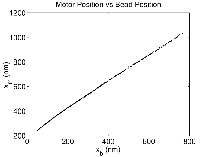
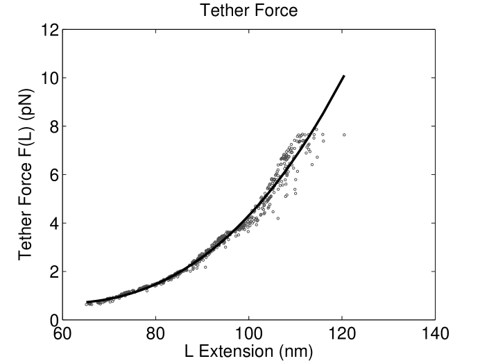
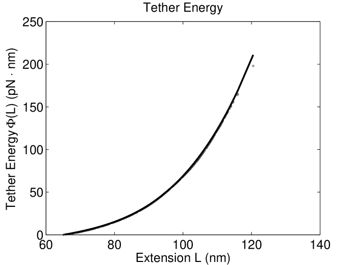
These two conditions allow for all of the data obtained under the three experiments in the  (svobodaandblock1994, ) paper to be mapped to equivalent observations under the experiment with an optical trap formed from a $15\mbox{mW}$ laser. The reconstruction method discussed in the previous section can then be applied to obtain the force-extension profile from the composite experimental data. The composite data of  (svobodaandblock1994, ) is plotted in figure 5. The reconstructed motor position, force-extension profile, and energy-extension profile are plotted in the figures 6, 7, 8, respectively.

Fig. 4: Diagram of the Optical Trap Experimental Setup for the Bead-Motor Tether. The center of the optical trap $x_{tr}$ is positioned so that the bead is in contact with the microscope stage. The center of the bead $x_{b}$ in the direction of the microtubule is observed as the stage is moved. The tether connecting the center of the bead to the motor at position $x_{m}$ is extended under the restoring force of the optical trap which is proportional to $x_{b}-x_{tr}$. The angle at which the tether is connected to the bead with respect to the direction parallel to the microscope stage is denoted by $\theta$. Note that the tether itself only consists of the segment from the motor to the surface of the bead and has the same binding angle as that illustrated. We also remark that by the geometry of the setup the extension of the tether only depends on $x_{m}-x_{b}$.

Fig. 5: Composite Experimental Data. In the plot (+) points were obtained with $15\mbox{mW}$ laser power, (o) with $30\mbox{mW}$, and (x) $62\mbox{mW}$ laser power. The data is from  (svobodaandblock1994, ) and are replotted here on a single graph by making use of the transformation explained in the text.

Fig. 6: Reconstructed Motor Position. The black points show the reconstructed motor position $x_{m}$ as a function of the experimentally observed bead position $x_{b}$ obtained by the integration procedure described in the text.

Fig. 7: Tether Force-Extension Profile. The plotted points are the reconstructed force-extension profile obtained from the procedure described in the text. The solid curve is a cubic polynomial with coefficients fit by the method of least-squares to the reconstructed force-extension profile of the tether. For small tether extensions in the model the force-extension profile is linearly interpolated to zero as the extension approaches zero.

Fig. 8: Tether Energy-Extension Profile. The plotted points are the reconstructed tether energy-extension profile obtained by numerical integration of the reconstructed tether force-extension profile. The solid curve is the analytic anti-derivative of the cubic polynomial obtained using a least-squares fit to the tether force-extension profile.

3 The Kinetic Cycle of the Model

In the model we postulate that the heads of the motor protein can be in any of three states which are represented by their binding affinity for the microtubule. The states are: bound to a microtubule (B), detached and diffusing with weak affinity for the microtubule (W), detached and diffusing with strong affinity for the microtubule (S). The overall state of the motor protein is then given by the binding states of each of the heads and the location of the bound head closest to the negative end of the microtubule. For clarity in the notation we shall suppress explicit mention of the bound head location.

Since we are primarily interested in the force dependent statistics of the optical trap experiments we shall restrict attention only to the states of the motor where one head is bound to the microtubule at all times. In the description of the model we shall not distinguish between the individual identity of the two heads but rather only represent their relative configuration. From these considerations the states of the motor are always in the set $\{BB,WB,BW,SB,BS\}$.

The kinetics of the model are specified by transitions between these states. For many of the states a transition will occur only after an exponentially distributed waiting time parameterized by a rate constant. The rate constant characterizes the probability per unit time that a transition event occurs. If we denote the rate constant by $\lambda$ the waiting time is a random variable $\tau$ with the probability density  (ross1995, )

$$\rho(t)=\lambda e^{-\lambda{t}}$$ (12)

In the model we do not commit to a specific correspondence between the proposed states and the ATP hydrolysis cycle. However, to motivate the model we will relate our state transitions to a kinetic scheme similar to that proposed in  (cross2004, ),  (cross2000, ).

In the following description, when both heads of kinesin are bound to the microtubule, we shall refer to the one closer to the plus end of the microtubule as the leading head and the one closer to the minus end of the microtubule as the trailing head. When only one head is bound to the microtubule, we shall not use the terminology ”leading” or ”trailing” and simply refer to one as the bound head and the other as the unbound head.

Each head of kinesin has a catalytic site which is specialized for ATP hydrolysis. This site may be empty, occupied by ATP, occupied by ADP and $P_{i}$, or occupied by ADP only.

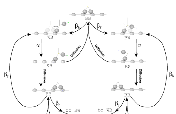
We begin the description of the hydrolysis cycle with one head bound and its hydrolysis site empty, and with the other head unbound and its hydrolysis site occupied by $ADP$. In fact, we assume that the $ADP$ molecule is trapped in the hydrolysis site of the unbound head and that it cannot be shed until other events occur that allow it to be released. This will be discussed shortly. We refer to this state as $WB$, meaning that one head is bound to the microtubule and the other head is not bound and has only weak affinity for the microtubule, see figure 9. In particular, the unbound head will remain unbound, with $ADP$ trapped in its hydrolysis site, as long as kinesin remains in this state.

The next step in the cycle is the binding of $ATP$ to the bound head of kinesin. Recall that the hydrolysis site of the bound head was empty and available to bind $ATP$. This is followed by $ATP$ hydrolysis in the bound head. We assume that one or the other of these reactions, either the binding of $ATP$ or the subsequent hydrolysis, is rate limiting and assign it the rate constant $\alpha$. The obvious result of this step is that the bound head now has $ADP$ and $P_{i}$ in its hydrolysis site, but we assume that a further result is a change in conformation of the kinesin molecule as a whole that makes the unbound head bind $ADP$ less strongly, and allows the unbound head to interact strongly with the microtubule.

As a result of the above, kinesin is now in the state $SB$, in which the unbound head will bind to the first empty kinesin-binding site on the microtubule that it encounters. The fast process of finding this binding site is diffusion-limited, and therefore is not described by a rate constant. We obtain the statistics of this transition by direct simulation of the stochastic dynamics of our mechanical kinesin model.

When the unbound but strongly interacting head encounters a kinesin binding site on the microtubule it binds there. The resulting conformational change in the kinesin molecule as a whole causes the shedding of $P_{i}$ from the other head, the one that was already bound, which is the one on which hydrolysis has most recently occurred.

At this point we have both heads bound, so the state of kinesin is $BB$, and both heads have $ADP$ in their hydrolysis sites. This situation is somewhat unstable, since the presence of $ADP$ in the hydrolysis site weakens the interaction with the microtubule. What happens next is that one of the two heads sheds its ADP. The head that does so binds more strongly to the microtubule, while the other head simultaneously lets go of the microtubule and binds more strongly to its $ADP$, trapping the $ADP$ in its hydrolysis site. The kinesin molecule is now in the state $WB$ with which we began the description of the hydrolysis cycle.

It is important to note, however, that there are two ways the above coordinated reaction, release of $ADP$ from one head, and disassociation of the other head from the microtubule, can occur, since the head that detaches from the microtubule can be the leading head or the trailing head. An important assumption of our model is that the rate constants for these two reactions are not the same. We call $\beta_{b}$ the rate constant for detachment of the trailing ”back” head from the microtubule, and $\beta_{f}$ the, much smaller, rate constant for detachment of the leading ”front” head from the microtubule. Whichever head detaches, though, carries $ADP$ trapped in its hydrolysis site, while the head that remains bound is left with its hydrolysis site empty.

Kinesin hydrolyzes on average one ATP molecule per step along the microtubule  (coy1999, ) and can move against load forces as great as $5-7pN$  (svobodaandblock1994, ). The hydrolysis of only one ATP per step suggests there must be a mechanism that drives the motor forward other than the asymmetric unbinding rates $\beta_{b}$ and $\beta_{f}$ of the front and back heads. If there were no other mechanism involved we would have by mechanical symmetry that a head detaching from the back microtubule site would have at least a $50$% probability of rebinding again to the back microtubule site. As a consequence each observed mechanical step would on average require consumption of more than one molecule of $ATP$.

To avoid this problem we introduce into the model a mechanical asymmetry. It has been reported in  (rice1999, ),  (rice2003, ) that when ATP binds the motor domain a loop of about 15 amino acid residues undergoes a disordered to ordered transition. This structure attaches the motor domains to the coiled-coiled stalk and is referred to as the “neck-linker”. In the ordered state the residues of the loop form a partial beta sheet structure close to the motor domain. In the model the effect of the neck-linker is accounted for by a harmonic spring acting on the hinge point which introduces a preferred configuration in the direction of the plus end of the microtubule when $ATP$ is in the hydrolysis site of the bound head. This biases the diffusion of the back head toward the front binding site.

Further refinements of the model may be possible incorporating mechanical information about the interactions of the neck-linker with the motor domains in  (rice1999, ),  (rice2003, ). It may also be possible to include the mechanism proposed by  (mogilner2001, ), which involves a competition between a docked and undocked state of the neck-linker, by introducing a bistable potential energy for the hinge point. However, inclusion in the model of a potential energy with multiple minima complicates the statistical sampling of the mechanical configurations. We leave these possible refinements to future work. The kinetic cycle and mechanics of the model are summarized in figure 9.

Fig. 9: State Transition Diagram for the Model. Each level denotes a state combination for the pair of Kinesin heads. The arrows represent admissible transitions that can be made in the model. Transitions that occur after an exponentially distributed waiting time are labeled with a rate constant. Transitions that occur only after a diffusive search of the free head has successfully found an available binding site are labeled by “diffusion”.

4 Simulation of the Model and Computation of Experimentally Measured Statistics

From the measurements of optical trap experiments, two statistics are typically published in the literature. These are (i) the average velocity at which the cargo bead is transported by the motor protein and (ii) the randomness parameter $q$ of the stochastic stepping process.

If we let $z_{t}$ be the component of the bead position along the axis of the microtubule at time $t$ then the average velocity of the bead is given by

$$v=\lim_{t\rightarrow\infty}\frac{E[z_{t}]}{t}$$ (13)

where $E[\cdot]$ denotes the ensemble expectation obtained by averaging the measurements over repeated experiments.

The randomness parameter $q$ is defined as

$$q=\lim_{t\rightarrow\infty}\frac{\mbox{var}[z_{t}]}{\mbox{E}[z_{t}]\cdot{\delta}}$$ (14)

where $\mbox{var}[\cdot]$ is the ensemble variance obtained by averaging over repeated experimental measurements, and $\delta=8$-nm is the spacing between microtubule binding sites.

The motivation for the randomness parameter comes from a process with elementary chemical events having exponentially distributed waiting times with identical rate constants $\lambda$. If each mechanical $8$-nm step requires $n$ elementary chemical events then a relatively straight-forward calculation using the Poisson distribution for the number of elementary events which have occurred for the motor before the time $t$ gives $q=\frac{1}{n}$. When the rates are not exactly the same the randomness parameter estimates the number of slow “rate limiting” events  (svoboda1994b, ).

In a rough sense the quantity $q$ measures the “randomness” of the process. If the number of chemical events per mechanical step is large $n\rightarrow\infty$ with the average time $t_{0}=\frac{n}{\lambda}$ for a mechanical step held constant for each $n$, then the waiting time distribution of the mechanical step approaches the Dirac $\delta$-distribution with unit mass centered at the time $t_{0}$. Thus as $q\rightarrow 0$ the mechanical stepping becomes increasingly like that of a deterministic stepping process with delay $t_{0}$ between steps.

In the experiments the bead is attached through the cargo tether to an active Kinesin motor protein. The position of the transported bead is measured with nanometer spatial accuracy and microsecond temporal accuracy. At the laser powers used in the experiments which we shall consider, the optical restoring force toward the center of focus can be approximated to a good degree by a Hookean spring where the restoring force is a linear function of the displacement. In many of the experiments the laser powers are sufficiently weak that many steps of the motor are required before the restoring force acting on the bead changes significantly. The load force varies only over relatively large length scales in comparison to the $8$-nm step of Kinesin protein.

To estimate the load force dependence of the motor in the experiments, the time series of the bead position is divided into small segments which are determined by when the bead is within a small range of displacements from the optical trap center. On each segment the statistics are computed by treating the load force as approximately constant. Some of the experiments employ a more sophisticated approach and use a feedback loop to move the optical trap as the motor progresses. This ensures that a fixed distance is maintained between the optical trap center and the bead and makes the load force to a high precision constant  (visscher1999, ).

A challenge in modeling the force dependent statistics is that we must be able to efficiently sample the behavior of the model over many steps of the motor protein and over a range of load forces. A further challenge arises from the range of time scales associated with the chemical kinetics and mechanics of the motor protein. In general the computation of these force dependent statistics by directly simulating a detailed model of the experimental system is computationally expensive.

The approach we shall take is to simulate a coarse-grained model of Kinesin using a two step protocol that simulates the mechanical aspects of the model separately from the chemical kinetics of the model. The geometry of the model was discussed in detail in section 1. In this section we shall discuss primarily the dynamics of the model and the simulation method.

In the experiment the bead and motor protein are immersed in a solvent. Given the small length scale of the motor protein and the cargo bead the Reynolds number associated with the system is small. We shall model the dynamics of the model by an over-damped diffusion process where the $k^{th}$ mechanical degree of freedom $\mathbf{X}_{t}^{\{k\}}$ evolves according to a stochastic differential equation

$$d\mathbf{X}_{t}^{\{k\}}=-\frac{1}{\gamma_{k}}\nabla_{\mathbf{X}^{\{k\}}}V(\mathbf{X}_{t})dt+\sqrt{2D_{k}}d\mathbf{B}_{t}^{\{k\}}$$ (15)

The potential energy of the system is denoted by $V$ and depends on the configuration of the entire system, which is denoted by $\mathbf{X}_{t}$. The details are given in the appendix. Associated with each degree of freedom is an effective friction coefficient $\gamma_{k}$ which captures the dissipation of energy that occurs from the interaction of the solvent with the bead and the heads of Kinesin. The associated diffusion coefficient is given by Einstein’s relation, $D_{k}=\frac{K_{B}{T}}{\gamma_{k}}$, which captures the thermal energy that is imparted by the solvent to the bead and the heads of Kinesin  (reichl1998, ). The thermal force in the system is modeled by white noise which we express for the $k^{th}$ mechanical degree of freedom in terms of increments of the standard three dimensional Brownian motion $\mathbf{B}_{t}^{\{k\}}$, which are taken as independent for each $k$.  (oksendal2000, ).

The model is simulated numerically by using an Euler discretization of the stochastic differential equation  (platen1992, )

$$\mathbf{X}_{k}^{n+1}=\mathbf{X}_{k}^{n}-\frac{1}{\gamma_{k}}\nabla_{\mathbf{X}_{k}}V(\mathbf{X}^{n})\Delta{t}+Z_{k}^{n}$$ (16)

The $k^{th}$ mechanical degree of freedom at time $t_{n}$ is denoted by $X_{k}^{n}$. The thermal force acting over the time increment $\Delta{t}$ is captured by a Gaussian random variable $Z_{k}$ with mean 0 and variance $\sqrt{2D_{k}\Delta{t}}$.

In the scheme the excluded volume interactions between the bodies are taken into account by a rejection method. If a probabilistic step of the scheme results in a configuration of the system that violates the excluded volume constraint this step is rejected. A new set of random numbers are generated for the step until an acceptable configuration is produced.

From an abstract perspective, in which we view the dynamic trajectories as random variables drawn from the space of continuous functions, the rejection method is equivalent to drawing trajectories in the subspace of admissible configurations. The random variables are then distributed according to the conditional probability obtained from the Ito measure associated with the stochastic process restricted to the admissible subspace. Alternatively, from the point of view of the Ito diffusion process in the configuration space of the model, the rejection method is equivalent to imposing reflecting (no-flux) conditions on the boundary of the subspace of admissible configurations.

Direct simulation of the proposed model in order to generate the measurements used to estimate the force dependent statistics presents a difficulty. The estimated rate constants of the hydrolysis cycle yield waiting times between chemical events on the order of milliseconds. These waiting times are long in comparison to the time scale of the diffusive dynamics of the bead and the motor heads. If the positions of the bead and motor heads are resolved to $0.1$ nanometer precision the time step must be taken on the order of $10^{2}$-ns. This requires on the order of $10^{4}$ time steps per chemical event. This makes the generation of even a single trajectory of the model spanning a $100$ chemical events computationally expensive requiring on the order of $10^{6}$ time steps. While it is computationally expensive to perform a direct simulation of the model this disparity in the time scales of the chemical kinetics and mechanics can in fact be exploited.

An important feature of the model is that the only diffusion limited event that depends directly on the mechanics of the protein is the rebinding of the freely diffusing head when it is in the strong affinity state. While for the other chemically limited events the free head and the bead do diffuse, they do not influence the waiting for these events to occur. In addition, since the waiting time for the chemically limited events in the model is long, to a good approximation the bead and motor have a random configuration distributed according to the equilibrium distribution.

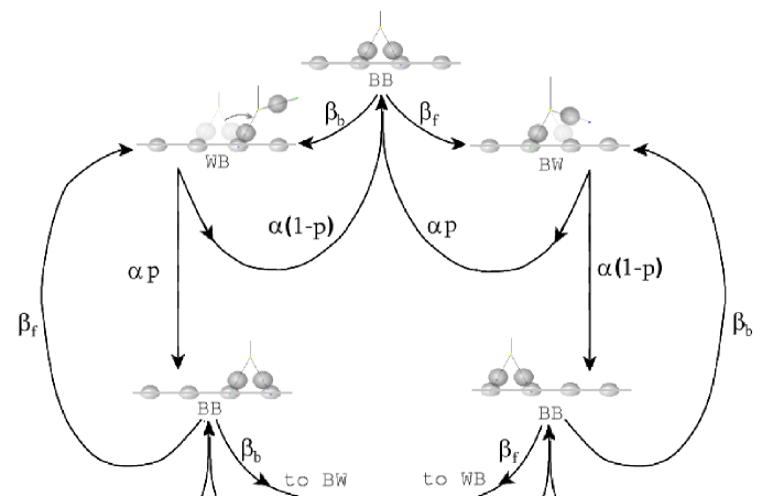
These insights allow for a simplification of the kinetic cycle of the model where the mechanical and chemical events of the motor protein can be essentially decoupled. Since the diffusive binding of the free head occurs on a time scale much faster than that of the chemical events, the transition $WB\rightarrow SB\rightarrow BB$ can be replaced by the single transition $WB\rightarrow BB$. The transition can be modeled by an effective rate constant $p\alpha$ for the event of the free head binding to the front site in the direction of the plus end of the microtubule and $(1-p)\alpha$ for binding to the back site. See figure 10 for a diagram of the kinetic cycle.

To simulate the model we use the following two step protocol:

(i) For a given load force generate a random configuration of the bead-motor system in the $WB$ state distributed according to the Boltzmann equilibrium distribution. For each sample simulate the diffusion process of the bead and motor until the free head binds to either the front or back site. From the simulations estimate the forward binding probability.

$$p(\mathbf{F})=\frac{\mbox{\# of times the free head binds the front site}}{\mbox{\# of times the free head binds either the front or back site}}$$ (17)

(ii) Simulate the simplified kinetic cycle using $p(\mathbf{F})$ from (i) for the $WB\rightarrow BB$ transition.

This approach yields substantial computational savings. The mechanics of the model need only be simulated over the relatively short time required for the free head to rebind the microtubule. Once $p$ has been determined the experimentally estimated statistics can be computed by simulating the simplified chemical kinetics of the model, which has now been reduced to a markov chain. To obtain a master equation we treat the identity of each of the heads as indistinguishable but do make a distinction at any moment between when a head is leading and when it is trailing. With this convention the master equation is

$$\frac{d[BB]_{j}}{dt} = p\alpha([WB]_{j}+[BW]_{j})+(1-p)\alpha[WB]_{j+1}+(1-p)\alpha[BW]_{j+1}$$

$$- (\beta_{b}+\beta_{f})[BB]_{j}$$

$$\frac{d[BW]_{j}}{dt} = \beta_{f}[BB]_{j}-\alpha[BW]_{j}$$

$$\frac{d[WB]_{j+1}}{dt} = \beta_{b}[BB]_{j}-\alpha[WB]_{j+1}$$

The first symbol of the pair is the state of the back head and the second symbol of the pair is the state of the front head. The subscript $j$ indicates the site index of the bound head closest to the minus end of the microtubule.

In the implementation of the method the Metropolis algorithm is used to generate the random initial configuration of the bead and motor in the $BW$ state.  (landau2000, ). The Forward-Euler rejection scheme proposed above is used to simulate the over-damped diffusive dynamics with excluded volume interactions until the free head rebinds the microtubule. The markov chain representing the kinetic cycle is simulated both directly by generating variates with exponentially distributed waiting times for each of the respective state transitions and by numerically solving the corresponding master’s equations 4 - 4.

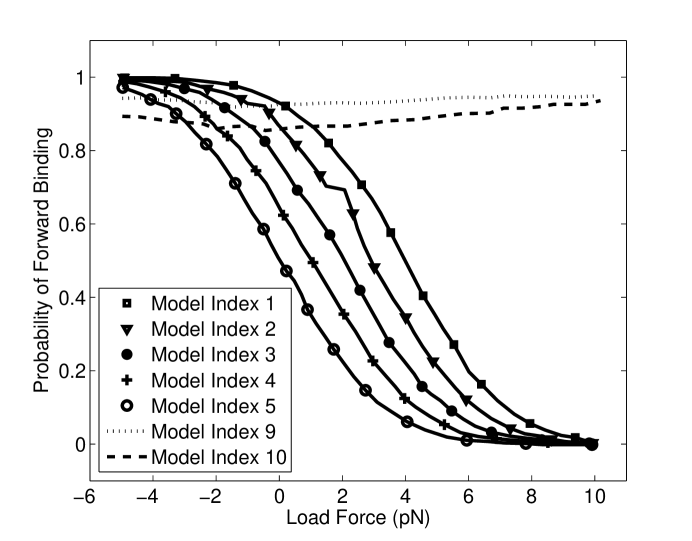
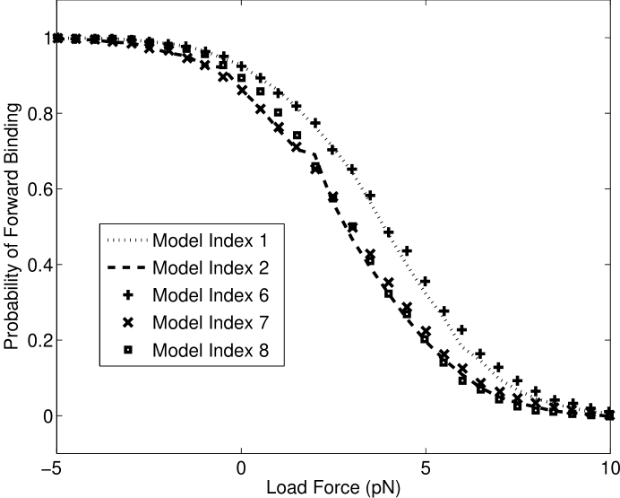
In figures 11, 12 the front site binding probability $p(\mathbf{F})$ is computed by varying a subset of the model parameters. See tables 1, 2, 3, 4 for more details.

Fig. 10: State Transition Diagram of the Model with the Free Head Fast Diffusion Approximation. Each level depicts a state combination for the pair of Kinesin heads. The arrows denote the admissible transitions of the model. Each transition occurs after an exponentially distributed waiting time with the corresponding rate constant denoted by the label. The state $BS$ has been eliminated from the model by the fast diffusion approximation and the transitions from $WB\rightarrow BS\rightarrow BB$ have been approximated by the transitions of the form $WB\rightarrow BB$ with rate constants $\alpha p$ and $\alpha(1-p)$. The factor $p=p(\mathbf{F})$ denotes for a given load force $\mathbf{F}$ the probability that the free head binds to the site on the microtubule toward the plus end.

Table 1: The Parameters of the Three Dimensional Kinesin Model

Parameter	Description
$K_{B}$	Boltzmann’s constant
$T$	Temperature
$L$	Spacing between the binding sites.
$R_{bindingSite}$	Radius of the binding sites.
$R_{bead}$	Radius of the bead.
$K_{m}$	Stiffness of the springs connecting the heads
	to the hinge point.
$R_{m}$	Rest length of the spring connecting
	the heads to the hinge.
$R_{glb}$	Radius of the spherical excluded volume of
	each head.
$\{a_{k}\}_{k=0}^{3}$	Coefficients of the cubic fit to the tether
	force-extension data.
$\mathbf{K}_{bias}$	Stiffness for the restoring force of the hinge bias.
$\mathbf{x}_{0}$	Displacement of the power stroke with the hinge point
	having the preferred position $\mathbf{X}_{bound}+\mathbf{x}_{0}$.
$\beta_{b}$	Back head unbinding rate $BB\rightarrow WB$.
$\beta_{f}$	Forward head unbinding rate $BB\rightarrow BW$.
$\alpha$	Weak affinity to strong affinity transition
	rate $WB\rightarrow SB$.
$\mathbf{X}_{\mbox{bead}}$	Bead position.
$\mathbf{X}_{\mbox{hinge}}$	Hinge position.
$\mathbf{X}_{\mbox{h1}}$	Microtubule binding site interaction point
	of head 1 position.
$\mathbf{X}_{\mbox{h2}}$	Microtubule binding site interaction point
	of head 2 position.
$\mathbf{F}$	Load force acting on the bead.

Table 2: Parameter Values for the Three Dimensional Model: The values given here are the default values for the model when we consider variations of any subset of the parameters.

Parameter	Value
$K_{B}$	$4.142\mbox{pN$\cdot$nm}$
T	$300\mbox{K}$
$L$	8 nm
$R_{bindingSite}$	2 nm
$R_{bead}$	$250\mbox{nm}$
$K_{m}$	$\frac{K_{B}{T}}{(\frac{L}{3})^{2}}=0.5825\mbox{pN/nm}$
$R_{m}$	$8\mbox{nm}$
$R_{glb}$	$2\mbox{nm}$
$\{a_{k}\}_{k=0}^{3}$	$\begin{array}[]{ll}a_{0}=3.4287,&a_{1}=-0.0372\\ a_{2}=-0.0010,&a_{3}=1.5050\times 10^{-5}\\ \end{array}$
$\mathbf{K}_{bias}^{(1)}$	$1\mbox{pN/nm}$
$\mathbf{K}_{bias}^{(2)}$	$1\mbox{pN/nm}$
$\mathbf{K}_{bias}^{(3)}$	$0\mbox{pN/nm}$
$\mathbf{x}_{0}^{(1)}$	$4\mbox{nm}$
$\mathbf{x}_{0}^{(2)}$	$0\mbox{nm}$
$\mathbf{x}_{0}^{(3)}$	$0\mbox{nm}$
$\beta_{b}$	$102.5\mbox{s}^{-1}$
$\beta_{f}$	$2.5\mbox{s}^{-1}$
$\alpha$	$400\mbox{s}^{-1}$

Table 3: Description of the Simulations of the Three Dimensional Model

Model Index	Description
1	Forward bias of $x_{0}^{(1)}=4$.
2	Parameters chosen to match one dimensional
	model when possible with $x_{0}^{(1)}=3$.
3	Forward bias of $x_{0}^{(1)}=2$.
4	Forward bias of $x_{0}^{(1)}=1$.
5	No forward bias $x_{0}^{(1)}=0$.
6	Linear spring used instead of cubic model
	of the tether with $x_{0}^{(1)}=4$.
7	Linear spring used instead of cubic model
	of the tether with $x_{0}^{(1)}=3$.
8	Lacks excluded volume and has forward bias of $x_{0}^{(1)}=3$.
9	Sideways force applied to model with $x_{0}^{(1)}=4$.
10	Sideways force applied to model with $x_{0}^{(1)}=3$.

Table 4: Parameter Values used for each Simulation of the Three Dimensional Model

Model Index	$x_{0}^{(1)}$	Excluded Volumes	Tether Type	Force Direction
1	4	yes	cubic	opposed
2	3	yes	cubic	opposed
3	2	yes	cubic	opposed
4	1	yes	cubic	opposed
5	0	yes	cubic	opposed
6	4	yes	linear	opposed
7	3	yes	linear	opposed
8	3	no	cubic	opposed
9	4	yes	cubic	sideways
10	3	yes	cubic	sideways

Fig. 11: Probability of Binding the Forward Site. The function $p=p(\mathbf{F})$ denotes for a given load force $\mathbf{F}$ the probability that the free head binds to the site of the microtubule toward the plus end. The sigmoidal curves plot the probability function verses the load force in the direction of the minus end of the microtubule with signed magnitude. Thus positive load forces oppose the motor and negative load forces push in the preferred direction of the motor. The curves left to right plot $p(\mathbf{F})$ when the forward leaning biasing parameter of the model is set to $x_{0}^{(1)}=0,1,2,3,4$ respectively. The two nearly horizontal curves near the top of the figure plot the forward binding probability when the load force is taken in the direction orthogonal to the microtubule and parallel to the microscope stage.

Fig. 12: Probability of Binding the Forward Site. The solid sigmoidal curves left to right in the model are with forward biasing parameter set to $x_{0}^{(1)}=3,4$ respectively. The curves with the symbols $+$ and $\times$ denote the probability of binding the forward site when the nonlinear spring that models the tether is changed to an approximating linear spring. The curves with the symbols $\Box$ denote the probability of binding the forward site when the excluded volume interactions are neglected in the model. In all of the plots the load force is taken in the direction of the minus end of the microtubule with signed magnitude as described in the previous figure.

5 Comparison with Optical Trap Data

In this section we compare the simulation results with the experimental data of  (svobodaandblock1994, ),  (block2003, ),  (coppin1997, ), and  (visscher1999, ). We also compare the three dimensional model proposed here with its one-dimensional linear-spring counterpart proposed in  (peskin1995, ).

Before making these comparisons we should remark that the experimental data available for the motor protein Kinesin is of a somewhat limited nature. For example significant differences appear in the literature for published data of experiments under similar conditions. In  (coppin1997, ) and  (visscher1999, ) the force-velocity statistics are computed for Kinesin at a $5\mu\mbox{M}$ ATP concentration. As illustrated in the figure 15 the experimental data in the two experiments differ significantly especially in the range of negative load forces that push the motor in the direction of the plus end of the microtubule.

Some aspects of the experiment that may account for the discrepancies include the use of different optical trap techniques which may probe the features of the motor through the cargo bead differently and the use of different biological sources to obtain the Kinesin motor proteins. In  (visscher1999, ) the optical trap center is moved as the motor progresses to maintain an approximately fixed distance from the bead to obtain a constant load force to high precision. In  (coppin1997, ) the optical trap is formed at a fixed position.

As a result of these limitations the comparison we make with the experimental data is largely qualitative and primarily shows some of the changes in the motor statistics that can arise from the three dimensional mechanics of the motor. Our aim in comparing with the data is to show that the general features of the model are reasonable.

Fig. 13: Comparison of the Experimental Force-Velocity Data of  (svobodaandblock1994, ) at 1 mM with the Model. The data points with error bars are replotted from the paper of  (svobodaandblock1994, ). The dashed curve plots the force-velocity profile of the one dimensional Kinesin model proposed in  (peskin1995, ). The solid curve plots the force-velocity profile of the best fit of the three dimensional model proposed in this paper.

Fig. 14: Comparison of the Experimental Force-Velocity Data of  (block2003, ) at 1.6 mM with the Model. The data points with error bars are replotted from the paper of  (block2003, ). The dashed curve plots the force-velocity profile of the one dimensional Kinesin model proposed in  (peskin1995, ). The solid curve plots the force-velocity profile of the best fit of the three dimensional model proposed in this paper.

Fig. 15: Comparison of the Experimental Force-Velocity Data of  (coppin1997, ) and  (visscher1999, ) at $5\mu M$ with the Model. The data points with the $*$ symbol and error bars are replotted from the paper of  (visscher1999, ). The data points with the $\bullet$ symbol are replotted from the paper of  (coppin1997, ). The dashed curve plots the force-velocity profile of the one dimensional Kinesin model proposed in  (peskin1995, ). The solid curve plots the force-velocity profile of the best fit of the three dimensional model proposed in this paper.

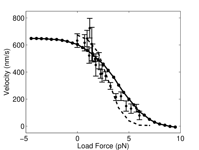
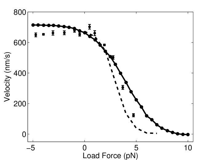
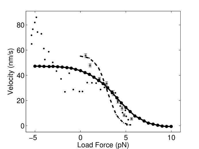
All of the experimental data was fit using the $p(\mathbf{F})$ computed in the previous section for the three dimensional model with index 1. Overall we find the model fit the data only moderately well. The data set with the most discrepancy was the force velocity statistics of  (coppin1997, ) in which the negative load force pushes the motor toward the plus end of the microtubule. As mentioned in the beginning of this section these data differ from  (visscher1999, ). Also in the experiment of  (block2003, ) the trend of an increasing velocity for the motor as the forward load force increases was not found. This suggests that there may be some features of the experimental techniques that can account for the difference, although it can not be ruled out that this may in fact be an intrinsic feature of the Kinesin motor proteins used in the experiment. For the data set of  (coppin1997, ) we fit the model to the experimental data sets in the range where they tended to agree with  (visscher1999, ).

We find that much of the experimental data for the force velocity statistic appears to fall in a range between the three dimensional model and one dimensional model. As discussed in the beginning of this section, the force velocity statistic of the model is proportional up to a translation to the function $p(\mathbf{F})$. The probability $p(\mathbf{F})$ of binding the forward site in the three dimensional model makes a more gradual transition from $1$ to $0$ as the load force increases than in the one dimensional model. This indicates that the probability of the free head binding a forward site is much more sensitive to the load force in the one dimensional model. One approach to reduce the discrepancy with the experimental data would be to construct a mechanical model of the motor protein for which the sensitivity of $p(\mathbf{F})$ to the load force falls between that of the proposed one dimensional and three dimensional models.

An alternative hypothesis to account for the discrepancy with the experimental data is that the parameters associated with the chemically regulated steps of the motor depend on the load force. Both of these aspects of the model can be adjusted to fit the force velocity statistic but additional experimental data, such as the measurement of the randomness parameter, places important constraints on how this may be done. One approach to distinguishing between these two alternatives is to require that the model fit the force variance or randomness parameter of the experiments.

In  (visscher1999, ) and  (block2003, ) the randomness parameter was computed experimentally. Below we show for the three dimensional model a fit performed simultaneously for the randomness parameter and the force velocity statistic of  (block2003, ). The fit to the force velocity statistic was shown in the previous figures.

Fig. 16: Comparison of the Experimental Data for the Randomness Parameter of  (block2003, ) at 1.6 mM and  (visscher1999, ) at 2 mM with the Model. The data points with the $+$ symbol and error bars are replotted from  (block2003, ). The data points with the $\bullet$ symbol and error bars are replotted from  (visscher1999, ). The solid curve plots the randomness profile of the three dimensional model proposed in this paper fit to the force-velocity data of  (block2003, ).

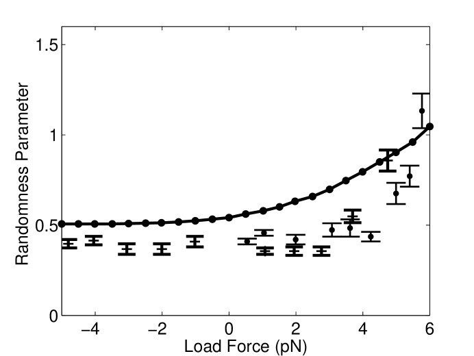
We find that the three dimensional model tends to have a higher randomness parameter but follows the same general trend. In the model there is a limit to how small the randomness parameter can become when the parameters of the model are nontrivial. The randomness parameter can be shown to have a minimum of $\frac{1}{2}$ when the probability of taking a forward step is one $p=1$. For most of the load forces the randomness parameter of the model is about $0.5$ and that of the experimental data is $0.4$. This suggests that there may be additional states of Kinesin not accounted for in the model that have collectively a non-negligible but moderately fast transition rate on the time scale of the chemically regulated steps of the model. For example if we include in the model the shedding of the hydrolysis product $P_{i}$ after $ATP$ binds one of the bound Kinesin heads it would be expected that this does not change many of the trends observed in the statistics of the model but this additional exponentially distributed waiting time would result in an overall lowering of the randomness parameter.

For the sideways load forces the predictions of the model do not agree with the trends observed experimentally. In the experimental observations of  (block2003, ) the velocity of the motor decreases as the sideways load increases. Interestingly, while contrary to the experimental observations of Kinesin the three dimensional mechanical model has a velocity that is found to increase slightly with sideways load forces.

6 Conclusion

In this paper we have derived from optical trap experimental data the force-extension profile of the coiled-coil tether than attaches cargo to the Kinesin motor protein. This was accomplished by formulating a theoretical model of the experiment that allows the extension and the restoring force of the tether to be deduced from the observations of the cargo bead position and the velocity ratio of the bead relative to the moving stage. We then proposed a three dimensional mechanical model of Kinesin incorporating the reconstructed force-extension profile into the model. Force dependent statistics were computed for the model by a procedure that exploits a separation of times scales between the diffusion time scales of the cargo bead and Kinesin heads and the time scales of the chemical kinetics of the motor. The statistics obtained were then compared with experimental data.

7 Acknowledgments

Both authors were supported by research grant R01 GM59875-01A1 from the National Institutes of Health. We are indebted to George Oster for introducing us to the problem of modeling Kinesin, and for helpful discussions in connection with this work.

Appendix

Potential Energy for the Mechanical Model

The potential energy for the entire system consists of

$$\mathbf{X} = \left[\mathbf{X}_{bead},\mathbf{X}_{hinge},\mathbf{X}_{h1},\mathbf{X}_{h2}\right]$$ (19)

$$V(\mathbf{X}) = V_{tether}+V_{hinge}+V_{motor}+V_{trap}$$

In this notation the three dimensional positions of the two heads of the Kinesin motor are denoted by $\mathbf{X}_{h1}$,$\mathbf{X}_{h2}$. The bead transported by the motor has position $\mathbf{X}_{bead}$. The position of the hinge point where the two heads join the tether of the motor is given by $\mathbf{X}_{hinge}$. In the model the energy is taken to be a function of only these four degrees of freedom and consists of contributions from the stretching of the tether, preferred hinge orientation, elasticity of the heads, and the optical trap.

The tether potential energy was derived from the experimental data as explained in section 2.2. The force-extension profile was found to be approximated well by a cubic polynomial with coefficients $\{a_{k}\}$. The tether energy is modeled consistently with the cubic fit by the following potential.

$$V_{tether} = E_{tether}(|\mathbf{X}_{b}-\mathbf{X}_{hinge}|)$$ (20)

$$E_{tether}(s) = \frac{a_{3}}{4}s^{4}+\frac{a_{2}}{3}s^{3}+\frac{a_{1}}{2}s^{2}+a_{0}s$$

In the model the free head is biased toward the plus end of the microtubule. This occurs through a force that has the tendency to keep the bound head at a fixed angle with the microtubule. We model this by linear springs in each spatial direction that tend to maintain the hinge position in a subset of preferred configurations. The biasing force is specified by a separate stiffness for each spatial component. We remark that in the model $K_{bias}^{(3)}$ has been set to zero in all of the simulations but is included here for generality.

$$V_{hinge} = \frac{K_{bias}^{(1)}}{2}|\mathbf{X}_{hinge}^{(1)}-(\mathbf{X}_{bound}^{(1)}+\mathbf{x}_{0}^{(1)})|^{2}$$

$$+ \frac{K_{bias}^{(2)}}{2}|\mathbf{X}_{hinge}^{(2)}-(\mathbf{X}_{bound}^{(2)}+\mathbf{x}_{0}^{(2)})|^{2}$$

$$+ \frac{K_{bias}^{(3)}}{2}|\mathbf{X}_{hinge}^{(3)}-(\mathbf{X}_{bound}^{(3)}+\mathbf{x}_{0}^{(3)})|^{2}$$

The elasticity of the globular domains of the motor protein that mediate the force between the microtubule interaction sites of the head and the hinge point is modeled by two linear springs that contribute the following energy to the potential of the system.

$$V_{motor} = \frac{K_{m}}{2}(|\mathbf{X}_{hinge}-\mathbf{X}_{h1}|-L)^{2}+\frac{K_{m}}{2}(|\mathbf{X}_{hinge}-\mathbf{X}_{h2}|-L)^{2}$$ (22)

In the simulations the force exerted by the optical trap is modeled by a constant load force $\mathbf{F}$ reflecting the small spatial range over which we are interested in the experimental setup. This potential is given by

$$V_{trap} = -\mathbf{F}\cdot{\mathbf{X}_{bead}}$$ (23)

References

- (1) Bruce Alberts, Alexander Johnson, Julian Lewis, Martin Raff, Keith Roberts, and Peter Walker, Molecular Biology of the Cell, Garland Publishing, 2002.
- (2) L. A. Amos, Focusing-in on microtubule, Current Opinion in Structural Biology, 10 (2000), pp. 236–241.
- (3) R. D. Astumian and I. Derenyi, A chemically reversible brownian motor: Application to kinesin and ncd, Biophysical Journal, 77 (1999), pp. 993–1002.
- (4) E. Berliner, Failure of a single-headed kinesin to track parallel to microtubule protofilaments, Nature, 373 (1995), pp. 718–721.
- (5) S.M. Block, C.L. Asbury, J.W. Shaevitz, and M.J. Lang, Probing the kinesin reaction cycle with a 2d optical force clamp, Proc. Natl. Acad. Sci. USA, 100 (2003), pp. 2351–2356.
- (6) C. Bustamante, D. Keller, and G. Oster, The physics of molecular motors, Acc. Chem. Res., 34 (2001), pp. 412–420.
- (7) R. B. Case, S. Rice, C. L. Hart, B. Ly, and R.D. Vale, Role of the kinesin neck linker and catalytic core in microtubule-based motility, Current Biology, 10 (2000), pp. 157–160.
- (8) Y. Chen, B. Yan, and R. J. Rubin, Fluctuations and randomness of movement of bead powered by a single kinesin molecule in a force-clamped motility array: Monte-carlo simulations, Biophysical Journal, 83 (2002), pp. 2360–2369.
- (9) C.M. Coppin, J. T. Finer, J. A. Spudich, and R. D. Vale, Detection of sub-8-nm movements of kinesin by high-resolution optica-trap microscopy, Proc. Natl. Acad. Sci. USA, 93 (1996), pp. 1913–1817.
- (10) C.M. Coppin, D.W. Pierce, L. Hsu, and R.D. Vale, The load dependence of kinesin’s mechanical cycle, Proc. Natl. Acad. Sci. USA, 94 (1997), pp. 8539–8544.
- (11) D. L. Coy, M. Wagenbach, and J. Howard, Kinesin takes one 8-nm step for each atp that it hydrolyzes, J. Biol. Chem., 274 (1999), pp. 3667–3671.
- (12) R. A. Cross, The kinetic mechanism of kinesin, TRENDS in Biochemical Sciences, 29 (2004), pp. 301–307.
- (13) R. A. Cross, I. Crevel, N. J. Carter, M. C. Alonso, K. Hirose, and L. A. Amos, The conformational cycle of kinesin, Phil. Trans. R. Soc. Lond. B, 355 (2000), pp. 459–464.
- (14) K. Downing and E. Nogales, Tubulin and microtubule structure, Current Opinion in Cell Biology, 10 (1998), pp. 16–22.
- (15) T. C. Elston and C. S. Peskin, The role of protein flexibility in molecular motor function: coupling diffusion in a tilted periodic potential, SIAM Journal of Applied Mathematics, 60 (2000), pp. 842–867.
- (16) T. C. Elston, D. You, and C. S. Peskin, Protein flexibility and correlation ratchet, SIAM Journal of Applied Mathematics, 61 (2000), pp. 776–791.
- (17) M. E. Fisher and A. B. Kolomeisky, Simple mechanochemistry describes the dynamics of kinesin molecules, PNAS, 98 (2001), pp. 7748–7753.
- (18) R. F. Fox, Rectified brownian movement in molecular and cell biology, Physical Review E, 57 (1998), pp. 2177–2203.
- (19) S. Gilbert and K. Johnson, Pathway of processive atp hydrolysis by kinesin, Nature, 373 (1995), pp. 671–676.
- (20) L. S. B. Goldstein, Molecular motors: from one motor many tails to one motor many tales, TRENDS in Cell Biology, 11 (2001), pp. 477–482.
- (21) A. Hoenger, M. Thormahlen, R. Diaz-Avalos, M. Doerhoefer, K. N. Goldie, J. Muller, and E. Mandelkow, A new look at the microtubule binding patterns of dimeric kinesins, Journal of Molecular Biology, 297 (2000), pp. 1087–1103.
- (22) J. Howard, Mechanics of Motor Proteins and the Cytoskeleton, Sinauer Associates, 2001.
- (23) F. Julicher, A. Ajdari, and J. Prost, Modeling molecular motors, Reviews of Modern Physics, 69 (1997), pp. 1269–1281.
- (24) A. Kamal and L SB Goldstein, Principles of cargo attachments to cytoplasmic motor proteins., Current Opinion Cell Biology, 14 (2002), pp. 63–68.
- (25) E. Karsenti and I. Vernos, The mitotic spindle: a self-made machine, Science, 294 (2001), pp. 543–547.
- (26) M. Kikkawa, E. P. Sablin, Y. Okada, H. Yajima, R. J. Fletterick, and N. Hirokawa, Switch-based mechanisms of kinesin motors, Nature, 411 (2001), p. 439.
- (27) P. E. Kloeden and E. Platen, Numerical solution of stochastic differential equations, Springer-Verlag, 1992.
- (28) A. E. Knight and J. E. Molloy, Coupling atp hydrolysis to mechanical work, Nature Cell Biology, 1 (1999), pp. E87–E89.
- (29) F. Kozielski, S. Sack, A. Marx, M. Thormahlen, E. Schonbrum, V. Biou, A. Thompson, E. M. Mandelkow, and E. Mandelkow, The crystal structure of dimeric kinesin and implications for microtubule-dependent motility, Cell, 91 (1997), p. 985.
- (30) F. J. Kull, E. P. Sablin, R. Lau, R. J. Fletterick, and R. D. Vale, Crystal structure of the kinesin motor domain reveals a structural similarity to myosin, Nature, 380 (1996), pp. 550–555.
- (31) D. Landau and K. Binder, A Guide to Monte-Carlo Simulations in Statistical Physics, Cambridge University Press, 2000.
- (32) J. Li, K.K. Pfister, S. Brady, and A. Dahlstrom, Axonal transport and distribution of immunologically distinct kinesin heavy chains in rat neurons, Journal of Neuroscience Research, 58 (1999), pp. 226–241.
- (33) C. Maes and Maarten H. van Wieren, A markov model for kinesin, Journal of Statistical Physics, 112 (2003), pp. 329–355.
- (34) E. Mandelkow and A. Hoenger, Structures of kinesin and kinesin-microtubule interactions, Current Opinion in Cell Biology, 11 (1999), pp. 34–44.
- (35) A. Mogilner, A.J. Fisher, and R.J. Baskin, Structural changes in the neck linker of kinesin explain the load dependence of the motor’s mechanical cycle, Journal of Theoretical Biology, 211 (2001), pp. 143–157.
- (36) M. Nishiyama, E. Muto, Y. Inoue, T. Yanagida, and H. Higuchi, Substeps within the 8nm step of the atpase cycle of single kinesin molecules, Nature Cell Biology, 3 (2001).
- (37) E. Nogales, M. Whittaker, R.A. Milligan, and K.H. Downing, High-resolution model of the microtubule, Cell, 96 (1999), pp. 79–88.
- (38) B. Oksendal, Stochastic Differential Equations: An Introduction with Applications, Springer, 2000.
- (39) C. Peskin and G. Oster, Coordinated hydrolysis explains the mechanical behavior of kinesin, Biophysics J., 68 (1995), pp. 202–211.
- (40) C. S. Peskin, G. M. Odell, and G. F. Oster, Cellular motions and thermal fluctuations: The brownian ratchet, Biophysical Journal, 65 (1993), pp. 316–324.
- (41) S. Ray, E. Meyhöfer, R.A. Milligan, and J. Howard, Kinesin follows the microtubule’s protofilament axis, Journal of Cell Biology, 121 (1993), pp. 1083–1093.
- (42) L. E. Reichl, A modern course in statistical physics, John Wiley and Sons, 1998.
- (43) S. Rice, Y. Cui, S. Sindelar, N. Naber, M. Matuska, R. Vale, and R. Cooke, Thermodynamic properties of the kinesin neck-region docking to the catalytic core, Biophysical Journal, 84 (2003), pp. 1844–1854.
- (44) S. Rice, A. W. Lin, D. Safer, C.L. Hart, N. Naber, B.O. Carragher, S.M. Cain, E.. Pechatnikova, E. W. Wilson-Kubalek, M. Whittaker, E. Pate, R. Cooke, E. W. Taylor, R.A. Milligan, and R.D. Vale, A structural change in the kinesin motor protein that drives motility, Nature, 402 (1999), pp. 778–784.
- (45) S. Ross, Stochastic Processes, Wiley Text Books, 1995.
- (46) E. P. Sablin and R. J. Fletterick, Nucleotide switchets in molecular motors: structural analysis of kinesins and myosins, Current Opinion in Structural Biology, 11 (2001), pp. 716–724.
- (47) S. Sack, J. Muller, A. Marx, M. Thormahlen, E. M. Mandelkow, S. T. Brady, and E. Mandelkow, X-ray structure of motor and neck domains from rat brain kinesin, Biochemistry, 36 (1997), p. 16155.
- (48) M. Schliwa and G. Woehlke, Switching on kinesin, Nature, 411 (2001), pp. 424–425.
- (49) D. Sharp, G. Rogers, and J. Scholey, Microtubule motors in mitosis, Nature, 407 (2000), pp. 41–45.
- (50) C.V. Sindelar, M.J. Budny, S. Rice, N. Naber, R. Fletterick, and R. Cooke, Two conformations in the human kinesin power stroke defined by x-ray crystallography and epr spectroscopy, Nature structural Biology, 9 (2002), pp. 844–848.
- (51) Y. H. Song, A. Marx, J. Muller, G. Woehlke, M. Schliwa, A. Krebs, A. Hoenger, and E. Mandelkow, Structure of fast kinesin: implications for atpase mechanisms and interactions with microtubules, Embo J., 20 (2001), p. 6213.
- (52) K. Svoboda and S. Block, Force and velocity measured for single kinesin molecules, Cell, 77 (1994), pp. 773–784.
- (53) K. Svoboda, P. Mitra, and S. Block, Fluctuation analysis of motor protein movement and single enzyme kinetics, Proc. Nat. Acad. Sci., (1994b).
- (54) K. Svoboda, C. F. Schmidt, B. J. Schnapp, and S. M. Block, Direct observation of kinesin stepping by optical trapping interferometry, Nature, 365 (1993), pp. 721–727.
- (55) C.M. Tuma, A. Zill, N. Le Bot, I. Vernos, and V. Gelfand, Heterotrimeric kinesin ii is the microtubule motor protein responsible for pigment dispersion in xenopus melanophores, The Journal of Cell Biology, 143 (1998), pp. 1547–1558.
- (56) R. Vale and R. Fletterick, The design plan of kinesin motors, Annu. Rev. Cell Dev. Biol., 13 (1997), pp. 745–777.
- (57) K. Visscher, M. Schnitzer, and S. M. Block, Single kinesin molecules studies with a molecular force clamp, Nature, 400 (1999), pp. 184–189.
- (58) G. Woehlke, A.K. Ruby, C.L. Hart, B. Ly, N. Hom-Booher, and R.D. Vale, Microtubule interaction site of the kinesin motor, Cell, 90 (1997), pp. 207–216.
- (59) M. Yun, C. E. Bronner, C. G. Park, S. S. Cha, H. W. Park, and S. A. Endow, Rotation of the stalk/neck and one head in a new crystal structure of the kinesin motor protein, J. Embo, 22 (2003), p. 1.