ITEP/TH-48/09

Notes on Chern-Simons Theory in the Temporal Gauge

Andrey Smirnov 111E-mail: asmirnov@itep.ru

Abstract

We analyze the perturbative series expansion of vacuum expectation values (vevs) for Wilson loop operators in Chern-Simons (CS) gauge theory in the temporal gauge A0=0subscript๐ด00A_{0}=0. Following J. Labastida and E. Pรฉrez we introduce the notion of the kernels of knot polynomial invariants - the (non-invariant) vevs of the Wilson loops, arising from CS theory in the temporal gauge. A method for exact calculation of the kernels of knot polynomial invariants is presented.

1 Introduction

In 1988, Edward Witten showed the connection between Chern-Simons field theory and the theory of knots in three-dimensional space [1]. Since that time the knot theory has been intensively studied using the standard quantum field theory methods. Different approaches inherent in quantum field theory established important connections between different types of knot invariants and provided a lot of new constructions for them.
The CS theory has been studied in different ways. Using series of non-perturbative methods Edward Witten in his original paper proved the equivalence of vacuum expectation values for Wilson lines operators and known polynomial knot invariants [2]-[6]. Perturbative studies performed in series of paper [7]-[15] established the connection between the coefficients of perturbative series expansion of vevs for Wilson loops and finite type (Vassiliev) knot invariants [17, 18].
Perturbative series expansion has been studied for different gauge fixing. The study of CS theory in the covariant Landau gauge performed in [7, 8] showed the equivalence of coefficients for the perturbative series and the integral representation for invariants by Bott and Taubes [19]. The Kontsevich integral representation for Vassiliev invariants turned out to correspond to the coefficients of vevs of Wilson lines operators in the light-cone gauge [14, 20].
In this paper we concentrate our attention on the study of CS theory in the temporal gauge. Different aspects of this gauge were discussed in [10, 13, 16]. In the temporal gauge A0=0subscript๐ด00A_{0}=0 the cubic term of the CS action disappears and the main ingredient for perturbative calculations is the gauge propagator. As it was noted in [13] the calculation of the gauge propagator in non-covariant gauges is plagued with ambiguities which should be solved by demanding additional properties for the correlation functions of gauge fields. As it was shown in [14] in non-covariant gauges we need to introduce some additional term to the propagator in order to obtain the knot invariants. Unfortunately, at present the correction term for the propagator in the temporal gauge is not known yet. In this paper we work with the propagator (6) without the correction term what leads to non-invariant quantities for vevs of the Wilson loop operators. On the other hand side as it was argued in [13] the propagator (6) contains enough information about a knot to reconstruct the full knot invariants in any order. Following the definitions of [13] we call these non-invariant vevs of Wilson loops the kernels of polynomial invariants.
The aim of this paper is to present the method for calculation of the kernels of the knot polynomial invariants in a very simple way. We show that there exists an operator X:R1โŠ—R2โ†’R1โŠ—R2:๐‘‹โ†’tensor-productsubscript๐‘…1subscript๐‘…2tensor-productsubscript๐‘…1subscript๐‘…2X:R_{1}\otimes R_{2}\rightarrow R_{1}\otimes R_{2}, where R1subscript๐‘…1R_{1} and R2subscript๐‘…2R_{2} are some representations of gauge group of CS action, such that the kernel of polynomial invariant for a knot with m๐‘šm intersection points can be obtained by appropriate contraction of indexes for m๐‘šm copies of the operator X๐‘‹X.
The structure of the article is as follows: in section 222 we discuss the main ingredients of perturbative calculations in CS theory for the temporal gauge and explain in details the calculation of vevs for Wilson loops in the simplest abelian case. In section 333 we discuss the geometrical Labastida-Pรฉrez formula for perturbative series expansion in non-abelian case and present some results of explicit calculations with this formula for the gauge group Gโ€‹Lโ€‹(N)๐บ๐ฟ๐‘GL(N). In section 444 we introduce a notion of the intersection operator, we calculate explicitly this operator for the case of Gโ€‹Lโ€‹(2)๐บ๐ฟ2GL(2) gauge group. As an example, using this operator we calculate the exact answer for kernel of polynomial invariant for the trefoil knot in Gโ€‹Lโ€‹(2)๐บ๐ฟ2GL(2) case.

2 Chern-Simons theory in the temporal gauge

2.1 The propagator of the gauge fields in the temporal gauge

Let G๐บG be a semi-simple Lie group and A=Aฮผaโ€‹(x)โ€‹dโ€‹xฮผโ€‹Fa๐ดsuperscriptsubscript๐ด๐œ‡๐‘Ž๐‘ฅ๐‘‘superscript๐‘ฅ๐œ‡superscript๐น๐‘ŽA=A_{\mu}^{a}(x)dx^{\mu}F^{a} be a G๐บG-connection on โ„3superscriptโ„3\mathbb{R}^{3}, where Fasuperscript๐น๐‘ŽF^{a} are the generators of Lie algebra of G๐บG in the fundamental representation. The Chern-Simons field theory is defined by the following action:

Sโ€‹[A]=โˆซโ„3tโ€‹rโ€‹(Aโˆงdโ€‹A+gโ€‹23โ€‹AโˆงAโˆงA)๐‘†delimited-[]๐ดsubscriptsuperscriptโ„3๐‘ก๐‘Ÿ๐ด๐‘‘๐ด๐‘”23๐ด๐ด๐ดS[A]=\int\limits_{\mathbb{R}^{3}}tr\left(\,A\wedge dA+g\,\dfrac{2}{3}\,A\wedge A\wedge A\,\right) (1)

where tโ€‹r๐‘ก๐‘Ÿtr denotes the trace over the fundamental representation of G๐บG and g๐‘”g is some parameter.
The CS theory is a particular example of a topological field theory [16], that implies that all the observables in this theory are some topological invariants. In this way, the CS theory is a natural tool for study of three-dimensional topology, for example the topology of three-dimensional knots. Indeed, let us consider the following gauge invariant operator associated with a knot cโˆˆโ„3๐‘superscriptโ„3c\in\mathbb{R}^{3}:

WRโ€‹(c)=tโ€‹rโ€‹(Pโ€‹expโก(gโ€‹โˆฎcAฮผaโ€‹(x)โ€‹Raโ€‹๐‘‘xฮผ)),subscript๐‘Š๐‘…๐‘๐‘ก๐‘Ÿ๐‘ƒ๐‘”subscriptcontour-integral๐‘superscriptsubscript๐ด๐œ‡๐‘Ž๐‘ฅsuperscript๐‘…๐‘Ždifferential-dsuperscript๐‘ฅ๐œ‡W_{R}(c)=tr\left(P\exp\left(g\oint\limits_{c}A_{\mu}^{a}(x)\,R^{a}\,dx^{\mu}\right)\right), (2)

this operator is just a Wilson loop associated with the knot c๐‘c or a trace of the holonomy of A๐ดA along the path c๐‘c. The index R๐‘…R means that one-form A๐ดA takes values in representation R๐‘…R of G๐บG. The natural class of the knot invariants provided by the CS theory is the vacuum expectation values of these operators:

<WRโ€‹(c)>=โˆซDโ€‹Aโ€‹expโก(โˆ’Sโ€‹[A])โ€‹WRโ€‹(c)expectationsubscript๐‘Š๐‘…๐‘๐ท๐ด๐‘†delimited-[]๐ดsubscript๐‘Š๐‘…๐‘<W_{R}(c)>=\int DA\exp(-S[A])\,W_{R}(c) (3)

In [1] E.Witten using non-perturbative methods showed that these invariants are in fact the well known polynomial knot invariants with the argument t=expโก(g2)๐‘กsuperscript๐‘”2t=\exp(g^{2}). To compute (3) using the standard perturbative methods (with respect to the parameter g๐‘”g) we need to chose a gauge fixing condition to make the associated functional integral well defined. Different choices of a gauge fixing lead to different descriptions of the same polynomial invariants [13, 14, 7]. The aim of this paper is to study the structure of the perturbative expansion of these polynomials in the so called temporal gauge. In the temporal gauge the condition imposed on the field A๐ดA is:

A0=0subscript๐ด00A_{0}=0

In this case the cubic term of the action (1) disappears and we arrive to a free field theory with the following action:

Sโ€‹[A]|A0=0=โˆซโ„3d3โ€‹xโ€‹Aฮผaโ€‹(ฮดaโ€‹bโ€‹ฯตฮผโ€‹โ€‰0โ€‹ฮฝโ€‹โˆ‚โˆ‚x0)โ€‹Aฮฝb,ฮดaโ€‹b=tโ€‹rโ€‹(Faโ€‹Fb)formulae-sequenceevaluated-at๐‘†delimited-[]๐ดsubscript๐ด00subscriptsuperscriptโ„3superscript๐‘‘3๐‘ฅsubscriptsuperscript๐ด๐‘Ž๐œ‡superscript๐›ฟ๐‘Ž๐‘superscriptitalic-ฯต๐œ‡โ€‰0๐œˆsubscript๐‘ฅ0subscriptsuperscript๐ด๐‘๐œˆsuperscript๐›ฟ๐‘Ž๐‘๐‘ก๐‘Ÿsuperscript๐น๐‘Žsuperscript๐น๐‘S[A]|_{A_{0}=0}=\int\limits_{\mathbb{R}^{3}}d^{3}x\,A^{a}_{\mu}\,(\,\delta^{a\,b}\,\epsilon^{\mu\,0\,\nu}\,\dfrac{\partial}{\partial x_{0}}\,)\,A^{b}_{\nu},\ \ \ \ \delta^{a\,b}=tr(F^{a}\,F^{b}) (4)

We have the following equation for the Green function:

ฮดaโ€‹bโ€‹ฯตฮผโ€‹โ€‰0โ€‹ฮฝโ€‹โˆ‚0โ–ณbโ€‹c,ฮฝโ€‹ฮทโ€‹(x)=ฮดaโ€‹cโ€‹ฮดฮผโ€‹ฮทโ€‹ฮดโ€‹(x)superscript๐›ฟ๐‘Ž๐‘superscriptitalic-ฯต๐œ‡โ€‰0๐œˆsubscript0superscriptโ–ณ๐‘๐‘๐œˆ๐œ‚๐‘ฅsuperscript๐›ฟ๐‘Ž๐‘superscript๐›ฟ๐œ‡๐œ‚๐›ฟ๐‘ฅ\delta^{a\,b}\,\epsilon^{\mu\,0\,\nu}\,\partial_{0}\,\triangle^{b\,c,\,\nu\,\eta}(x)=\delta^{a\,c}\,\delta^{\mu\,\eta}\,\delta(x)

for the solution of this equation we have (for careful derivation of this formula see [13]):

โ–ณbโ€‹c,ฮฝโ€‹ฮทโ€‹(x)=โˆ’ฯตฮฝโ€‹โ€‰0โ€‹ฮทโ€‹ฮดbโ€‹cโ€‹ฮดโ€‹(x1)โ€‹ฮดโ€‹(x2)โ€‹12โ€‹signโ€‹(x0)+fbโ€‹cโ€‹ฮฝโ€‹ฮทโ€‹(x1,x2),superscriptโ–ณ๐‘๐‘๐œˆ๐œ‚๐‘ฅsuperscriptitalic-ฯต๐œˆโ€‰0๐œ‚superscript๐›ฟ๐‘๐‘๐›ฟsubscript๐‘ฅ1๐›ฟsubscript๐‘ฅ212signsubscript๐‘ฅ0superscript๐‘“๐‘๐‘๐œˆ๐œ‚subscript๐‘ฅ1subscript๐‘ฅ2\triangle^{b\,c,\,\nu\,\eta}(x)=-\epsilon^{\nu\,0\,\eta}\,\delta^{b\,c}\,\delta(x_{1})\,\delta(x_{2})\,\dfrac{1}{2}\textrm{sign}(x_{0})+f^{b\,c\,\nu\,\eta}(x_{1},x_{2}), (5)

where fbโ€‹cโ€‹ฮฝโ€‹ฮทโ€‹(x1,x2)superscript๐‘“๐‘๐‘๐œˆ๐œ‚subscript๐‘ฅ1subscript๐‘ฅ2f^{b\,c\,\nu\,\eta}(x_{1},x_{2}) is an arbitrary tensor that does not depend on x0subscript๐‘ฅ0x_{0}. Particular choice of fbโ€‹cโ€‹ฮฝโ€‹ฮทโ€‹(x1,x2)superscript๐‘“๐‘๐‘๐œˆ๐œ‚subscript๐‘ฅ1subscript๐‘ฅ2f^{b\,c\,\nu\,\eta}(x_{1},x_{2}) depends on a prescription, some examples of different prescriptions can be found in [13, 16]. In this work we will restrict our attention to the case fbโ€‹cโ€‹ฮฝโ€‹ฮทโ€‹(x1,x2)=0superscript๐‘“๐‘๐‘๐œˆ๐œ‚subscript๐‘ฅ1subscript๐‘ฅ20f^{b\,c\,\nu\,\eta}(x_{1},x_{2})=0. In this case one obtains the following components of the propagator:

<A0a(x),Aฮผb(y)>=0,ฮผ=0,1,2;<Aฮผa(x),Aฮฝb(y)>=ฯตฮผโ€‹ฮฝฮดaโ€‹bฮด(x1โˆ’y1)ฮด(x2โˆ’y2)12sign(x0โˆ’y0),ฮผ,ฮฝ=1,2<\,A_{0}^{a}(x),\,A_{\mu}^{b}(y)\,>=0,\mu=0,1,2;\ \ \ <\,A_{\mu}^{a}(x),\,A^{b}_{\nu}(y)\,>=\epsilon^{\mu\,\nu}\,\delta^{a\,b}\,\delta(x_{1}-y_{1})\,\delta(x_{2}-y_{2})\,\dfrac{1}{2}\textrm{sign}(x_{0}-y_{0}),\ \ \mu,\nu=1,2 (6)

As we will see below, perturbation theory based on the propagator (6) leads to the quantities for <WRโ€‹(c)>expectationsubscript๐‘Š๐‘…๐‘<W_{R}(c)> that do not coincide with the known knot invariants obtained using non-perturbative methods and depend on a projection of the knot to the two-dimensional (x1,x2)subscript๐‘ฅ1subscript๐‘ฅ2(x_{1},x_{2}) plane. As it was conjectured in [13, 14] this deviation arises because we do not take into account the prescription depending term in (5).
Despite the vacuum expectation values of Wilson lines in this description are not knot invariants, they contain a lot of information about knots and as it was conjectured in [13] they can be used for a reconstruction of the full invariants. Following the notation of [13] we will denote these quantities by <W^Rโ€‹(c)>expectationsubscript^๐‘Š๐‘…๐‘<\hat{W}_{R}(c)> and call them kernels of polynomial invariants. The aim of this paper is to present the method that allows us to find exact expressions for the kernels of the polynomial invariants for every knot and for every representation in a very simple and elegant way.

2.2 The Abelian case as a basic example

Let us analyze in details the structure of the perturbative series expansion with propagator (6) in the Abelian case. In this case for the propagator we have:

ฮ ฮผโ€‹ฮฝ(xโˆ’y)=<Aฮผ(x),Aฮฝ(y)>=12ฯตฮผโ€‹ฮฝฮด(x1โˆ’y1)ฮด(x2โˆ’y2)sing(x0โˆ’y0),ฮผ,ฮฝ=1,2,A0=0\Pi_{\mu\,\nu}(x-y)=<\,A_{\mu}(x),\,A_{\nu}(y)\,>=\dfrac{1}{2}\epsilon^{\mu\,\nu}\,\delta(x_{1}-y_{1})\,\delta(x_{2}-y_{2})\,\textrm{sing}(x_{0}-y_{0}),\ \ \mu,\nu=1,2,\ \ \ A_{0}=0 (7)

The Wilson lines are presented by a โ€simpleโ€ exponents:

Wโ€‹(c)=expโก(gโ€‹โˆฎcAฮผโ€‹(x)โ€‹๐‘‘xฮผ)๐‘Š๐‘๐‘”subscriptcontour-integral๐‘subscript๐ด๐œ‡๐‘ฅdifferential-dsuperscript๐‘ฅ๐œ‡W(c)=\exp\left(g\,\oint\limits_{c}A_{\mu}(x)\,dx^{\mu}\right) (8)

We omit the label of representation because in the Abelian case the Wilson loop operators for different representations differ by a constant. For the perturbative expansion we get:

<W^(c)>=<โˆ‘n=0โˆž1n!(gโˆฎcAฮผ(x)dxฮผ)n>=โˆ‘n=0โˆž(2โ€‹nโˆ’1)!!2โ€‹n!g2โ€‹n(โˆซcโˆซcdxฮผdxฮฝ<Aฮผ(x),Aฮฝ(x)>)2โ€‹n<\hat{W}(c)>\,=\,<\sum_{n=0}^{\infty}\dfrac{1}{n!}\left(g\,\oint\limits_{c}A_{\mu}(x)\,dx^{\mu}\right)^{n}>=\,\sum_{n=0}^{\infty}\dfrac{(2n-1)!!}{2n!}g^{2n}\left(\int_{c}\int_{c}dx_{\mu}\,dx_{\nu}<A_{\mu}(x),A_{\nu}(x)>\right)^{2n}

and after the summation we obtain:

<W^โ€‹(c)>=expโก(g2โ€‹Lc)expectation^๐‘Š๐‘superscript๐‘”2subscript๐ฟ๐‘<\hat{W}(c)>\,=\exp\left(g^{2}\,L_{c}\right) (9)

where:

Lc=12โ€‹โˆซcโˆซc๐‘‘xฮผโ€‹๐‘‘yฮฝ<Aฮผโ€‹(x),Aฮฝโ€‹(y)>=12โ€‹โˆซcโˆซc๐‘‘xฮผโ€‹๐‘‘yฮฝโ€‹12โ€‹ฯตฮผโ€‹ฮฝโ€‹ฮดโ€‹(x1โˆ’y1)โ€‹ฮดโ€‹(x2โˆ’y2)โ€‹signโ€‹(x0โˆ’y0)formulae-sequencesubscript๐ฟ๐‘12subscript๐‘subscript๐‘differential-dsubscript๐‘ฅ๐œ‡differential-dsubscript๐‘ฆ๐œˆsubscript๐ด๐œ‡๐‘ฅsubscript๐ด๐œˆ๐‘ฆ12subscript๐‘subscript๐‘differential-dsuperscript๐‘ฅ๐œ‡differential-dsuperscript๐‘ฆ๐œˆ12superscriptitalic-ฯต๐œ‡๐œˆ๐›ฟsubscript๐‘ฅ1subscript๐‘ฆ1๐›ฟsubscript๐‘ฅ2subscript๐‘ฆ2signsubscript๐‘ฅ0subscript๐‘ฆ0L_{c}=\dfrac{1}{2}\int_{c}\int_{c}dx_{\mu}\,dy_{\nu}<A_{\mu}(x),A_{\nu}(y)>\,=\dfrac{1}{2}\int_{c}\int_{c}dx^{\mu}\,dy^{\nu}\dfrac{1}{2}\epsilon^{\mu\,\nu}\,\delta(x_{1}-y_{1})\,\delta(x_{2}-y_{2})\,\textrm{sign}(x_{0}-y_{0})

Let us parametrize the knot by a parameter t๐‘กt running from 00 to 111, then we can rewrite the last integral in the following form:

Lc=14โ€‹โˆซ01โˆซ01๐‘‘t1โ€‹๐‘‘t2โ€‹(dโ€‹x1dโ€‹t1โ€‹dโ€‹y2dโ€‹t2โˆ’dโ€‹x2dโ€‹t1โ€‹dโ€‹y1dโ€‹t2)โ€‹ฮดโ€‹(x1โ€‹(t1)โˆ’y1โ€‹(t2))โ€‹ฮดโ€‹(x2โ€‹(t1)โˆ’y2โ€‹(t2))โ€‹signโ€‹(x0โ€‹(t1)โˆ’y0โ€‹(t2))subscript๐ฟ๐‘14superscriptsubscript01superscriptsubscript01differential-dsubscript๐‘ก1differential-dsubscript๐‘ก2๐‘‘subscript๐‘ฅ1๐‘‘subscript๐‘ก1๐‘‘subscript๐‘ฆ2๐‘‘subscript๐‘ก2๐‘‘subscript๐‘ฅ2๐‘‘subscript๐‘ก1๐‘‘subscript๐‘ฆ1๐‘‘subscript๐‘ก2๐›ฟsubscript๐‘ฅ1subscript๐‘ก1subscript๐‘ฆ1subscript๐‘ก2๐›ฟsubscript๐‘ฅ2subscript๐‘ก1subscript๐‘ฆ2subscript๐‘ก2signsubscript๐‘ฅ0subscript๐‘ก1subscript๐‘ฆ0subscript๐‘ก2L_{c}=\dfrac{1}{4}\int_{0}^{1}\int_{0}^{1}dt_{1}dt_{2}\left(\dfrac{dx_{1}}{dt_{1}}\,\dfrac{dy_{2}}{dt_{2}}-\dfrac{dx_{2}}{dt_{1}}\,\dfrac{dy_{1}}{dt_{2}}\right)\delta(x_{1}(t_{1})-y_{1}(t_{2}))\,\delta(x_{2}(t_{1})-y_{2}(t_{2}))\,\textrm{sign}(x_{0}(t_{1})-y_{0}(t_{2}))

To perform the integration we need to solve the following equations:

{x1โ€‹(t1)โˆ’y1โ€‹(t2)=0x2โ€‹(t1)โˆ’y2โ€‹(t2)=0casessubscript๐‘ฅ1subscript๐‘ก1subscript๐‘ฆ1subscript๐‘ก20missing-subexpressionsubscript๐‘ฅ2subscript๐‘ก1subscript๐‘ฆ2subscript๐‘ก20\left\{\begin{array}[]{c}x_{1}(t_{1})-y_{1}(t_{2})=0\\ \\ x_{2}(t_{1})-y_{2}(t_{2})=0\end{array}\right. (10)

The solutions of these equations are the self-intersection points of two dimensional curve (x1โ€‹(t),x2โ€‹(t))subscript๐‘ฅ1๐‘กsubscript๐‘ฅ2๐‘ก(x_{1}(t),x_{2}(t)) which is the projection of the knot c๐‘c on the plane (x1,x2)subscript๐‘ฅ1subscript๐‘ฅ2(x_{1},x_{2}). Let us denote by t1k<t2ksuperscriptsubscript๐‘ก1๐‘˜superscriptsubscript๐‘ก2๐‘˜t_{1}^{k}<t_{2}^{k} the values of the parameter t๐‘กt in the intersection points, then the two-dimensional delta function in the integral can be represented in the form:

ฮดโ€‹(x1โ€‹(t1)โˆ’y1โ€‹(t2))โ€‹ฮดโ€‹(x2โ€‹(t1)โˆ’y2โ€‹(t2))=โˆ‘k(ฮดโ€‹(t1โˆ’t1k)โ€‹ฮดโ€‹(t2โˆ’t2k)+ฮดโ€‹(t1โˆ’t2k)โ€‹ฮดโ€‹(t2โˆ’t1k))|dโ€‹x1dโ€‹t1โ€‹dโ€‹y2dโ€‹t2โˆ’dโ€‹x2dโ€‹t1โ€‹dโ€‹y1dโ€‹t2|๐›ฟsubscript๐‘ฅ1subscript๐‘ก1subscript๐‘ฆ1subscript๐‘ก2๐›ฟsubscript๐‘ฅ2subscript๐‘ก1subscript๐‘ฆ2subscript๐‘ก2subscript๐‘˜๐›ฟsubscript๐‘ก1superscriptsubscript๐‘ก1๐‘˜๐›ฟsubscript๐‘ก2superscriptsubscript๐‘ก2๐‘˜๐›ฟsubscript๐‘ก1superscriptsubscript๐‘ก2๐‘˜๐›ฟsubscript๐‘ก2superscriptsubscript๐‘ก1๐‘˜๐‘‘subscript๐‘ฅ1๐‘‘subscript๐‘ก1๐‘‘subscript๐‘ฆ2๐‘‘subscript๐‘ก2๐‘‘subscript๐‘ฅ2๐‘‘subscript๐‘ก1๐‘‘subscript๐‘ฆ1๐‘‘subscript๐‘ก2\delta(x_{1}(t_{1})-y_{1}(t_{2}))\,\delta(x_{2}(t_{1})-y_{2}(t_{2}))=\sum\limits_{k}\dfrac{\left(\delta(t_{1}-t_{1}^{k})\delta(t_{2}-t_{2}^{k})+\delta(t_{1}-t_{2}^{k})\delta(t_{2}-t_{1}^{k})\right)}{|\dfrac{dx_{1}}{dt_{1}}\,\dfrac{dy_{2}}{dt_{2}}-\dfrac{dx_{2}}{dt_{1}}\,\dfrac{dy_{1}}{dt_{2}}|}

Substituting this expression into (10) and integrating over t1subscript๐‘ก1t_{1} and t2subscript๐‘ก2t_{2} we arrive to the following simple expression:

Lc=โˆ‘kฯตksubscript๐ฟ๐‘subscript๐‘˜subscriptitalic-ฯต๐‘˜L_{c}=\sum_{k}\epsilon_{k} (11)

where the quantities ฯตksubscriptitalic-ฯต๐‘˜\epsilon_{k} are the โ€singsโ€ of the intersection points. They can take values ยฑ1plus-or-minus1\pm 1 and are defined in the following way:

ฯตk=dโ€‹x1dโ€‹t1โ€‹(t1k)โ€‹dโ€‹y2dโ€‹t2โ€‹(t2k)โˆ’dโ€‹x2dโ€‹t1โ€‹(t1k)โ€‹dโ€‹y1dโ€‹t2โ€‹(t2k)|dโ€‹x1dโ€‹t1โ€‹(t1k)โ€‹dโ€‹y2dโ€‹t2โ€‹(t2k)โˆ’dโ€‹x2dโ€‹t1โ€‹(t1k)โ€‹dโ€‹y1dโ€‹t2โ€‹(t2k)|โ€‹signโ€‹(x0โ€‹(t1k)โˆ’y0โ€‹(t2k))subscriptitalic-ฯต๐‘˜๐‘‘subscript๐‘ฅ1๐‘‘subscript๐‘ก1superscriptsubscript๐‘ก1๐‘˜๐‘‘subscript๐‘ฆ2๐‘‘subscript๐‘ก2superscriptsubscript๐‘ก2๐‘˜๐‘‘subscript๐‘ฅ2๐‘‘subscript๐‘ก1superscriptsubscript๐‘ก1๐‘˜๐‘‘subscript๐‘ฆ1๐‘‘subscript๐‘ก2superscriptsubscript๐‘ก2๐‘˜๐‘‘subscript๐‘ฅ1๐‘‘subscript๐‘ก1superscriptsubscript๐‘ก1๐‘˜๐‘‘subscript๐‘ฆ2๐‘‘subscript๐‘ก2superscriptsubscript๐‘ก2๐‘˜๐‘‘subscript๐‘ฅ2๐‘‘subscript๐‘ก1superscriptsubscript๐‘ก1๐‘˜๐‘‘subscript๐‘ฆ1๐‘‘subscript๐‘ก2superscriptsubscript๐‘ก2๐‘˜signsubscript๐‘ฅ0superscriptsubscript๐‘ก1๐‘˜subscript๐‘ฆ0superscriptsubscript๐‘ก2๐‘˜\epsilon_{k}=\dfrac{\dfrac{dx_{1}}{dt_{1}}(t_{1}^{k})\,\dfrac{dy_{2}}{dt_{2}}(t_{2}^{k})-\dfrac{dx_{2}}{dt_{1}}(t_{1}^{k})\,\dfrac{dy_{1}}{dt_{2}}(t_{2}^{k})}{|\dfrac{dx_{1}}{dt_{1}}(t_{1}^{k})\,\dfrac{dy_{2}}{dt_{2}}(t_{2}^{k})-\dfrac{dx_{2}}{dt_{1}}(t_{1}^{k})\,\dfrac{dy_{1}}{dt_{2}}(t_{2}^{k})|}\,\textrm{sign}(x_{0}(t_{1}^{k})-y_{0}(t_{2}^{k})) (12)

Note that the expectation value (9) for the knot can be expressed in terms of product over the intersection points:

<W^โ€‹(c)>=โˆkexpโก(g2โ€‹ฯตk)expectation^๐‘Š๐‘subscriptproduct๐‘˜superscript๐‘”2subscriptitalic-ฯต๐‘˜<\hat{W}(c)>\,=\prod\limits_{k}\exp(g^{2}\,\epsilon_{k}) (13)

We see that the answer for vev in the abelian case has a form of a product over the intersection points of some quantity expโก(g2โ€‹ฯตk)superscript๐‘”2subscriptitalic-ฯต๐‘˜\exp(g^{2}\,\epsilon_{k}) that depends only on the intersection point. As we will see below in the non-abelian case this formula generalizes to the contraction of some tensors corresponding to intersection points.

3 The Non-Abelian Case

3.1 Labastida-Pรฉrez formula

In the case of non-Abelian gauge group the Wilson line operator is more complicated:

WRโ€‹(c)=trโ€‹Pโ€‹expโก(gโ€‹โˆฎcAฮผโ€‹(x)โ€‹๐‘‘xฮผ)subscript๐‘Š๐‘…๐‘tr๐‘ƒ๐‘”subscriptcontour-integral๐‘subscript๐ด๐œ‡๐‘ฅdifferential-dsuperscript๐‘ฅ๐œ‡W_{R}(c)=\textrm{tr}P\exp\left(g\,\oint\limits_{c}A_{\mu}(x)\,dx^{\mu}\right)

The vacuum expectation value has the form:

<Wโ€‹(c)>=โˆ‘m=0โˆžImRโ€‹(c)โ€‹g2โ€‹mexpectation๐‘Š๐‘superscriptsubscript๐‘š0superscriptsubscript๐ผ๐‘š๐‘…๐‘superscript๐‘”2๐‘š<W(c)>=\sum\limits_{m=0}^{\infty}I_{m}^{R}(c)g^{2m}

where the expansion are presented in terms of ordered multidimensional integrals:

ImRโ€‹(c)=tโ€‹rโ€‹(Ra1โ€‹Ra2โ€‹โ€ฆโ€‹Ram)โ€‹โˆซ01๐‘‘xฮผ1โ€‹โˆซ0xฮผ1๐‘‘xฮผ2โ€‹โ€ฆโ€‹โˆซ0xฮผmโˆ’1๐‘‘xฮผmโ€‹<Aฮผ1a1โ€‹Aฮผ2a2โ€‹โ€ฆโ€‹Aฮผmam>superscriptsubscript๐ผ๐‘š๐‘…๐‘๐‘ก๐‘Ÿsuperscript๐‘…subscript๐‘Ž1superscript๐‘…subscript๐‘Ž2โ€ฆsuperscript๐‘…subscript๐‘Ž๐‘šsuperscriptsubscript01differential-dsubscript๐‘ฅsubscript๐œ‡1superscriptsubscript0subscript๐‘ฅsubscript๐œ‡1differential-dsubscript๐‘ฅsubscript๐œ‡2โ€ฆsuperscriptsubscript0subscript๐‘ฅsubscript๐œ‡๐‘š1differential-dsubscript๐‘ฅsubscript๐œ‡๐‘šexpectationsuperscriptsubscript๐ดsubscript๐œ‡1subscript๐‘Ž1superscriptsubscript๐ดsubscript๐œ‡2subscript๐‘Ž2โ€ฆsuperscriptsubscript๐ดsubscript๐œ‡๐‘šsubscript๐‘Ž๐‘šI_{m}^{R}(c)=tr(R^{a_{1}}\,R^{a_{2}}...R^{a_{m}})\int_{0}^{1}dx_{\mu_{1}}\int_{0}^{x_{\mu_{1}}}dx_{\mu_{2}}...\int_{0}^{x_{\mu_{m-1}}}dx_{\mu_{m}}<A_{\mu_{1}}^{a_{1}}\,A_{\mu_{2}}^{a_{2}}...A_{\mu_{m}}^{a_{m}}>

where Rasuperscript๐‘…๐‘ŽR^{a} are the generators of the gauge group in a representation R๐‘…R. Using Wick theorem, and the following facts:

โˆซ01๐‘‘xฮผ1โ€‹โˆซ0xฮผ1๐‘‘xฮผ2โ€‹โ€ฆโ€‹โˆซ0xฮผmโˆ’1๐‘‘xฮผm=โˆซ๐‘‘x1โ€‹โ€ฆโ€‹๐‘‘xmโ€‹โˆk=1mโˆ’1ฮธโ€‹(xkโˆ’xk+1),superscriptsubscript01differential-dsubscript๐‘ฅsubscript๐œ‡1superscriptsubscript0subscript๐‘ฅsubscript๐œ‡1differential-dsubscript๐‘ฅsubscript๐œ‡2โ€ฆsuperscriptsubscript0subscript๐‘ฅsubscript๐œ‡๐‘š1differential-dsubscript๐‘ฅsubscript๐œ‡๐‘šdifferential-dsubscript๐‘ฅ1โ€ฆdifferential-dsubscript๐‘ฅ๐‘šsuperscriptsubscriptproduct๐‘˜1๐‘š1๐œƒsubscript๐‘ฅ๐‘˜subscript๐‘ฅ๐‘˜1\int_{0}^{1}dx_{\mu_{1}}\int_{0}^{x_{\mu_{1}}}dx_{\mu_{2}}...\int_{0}^{x_{\mu_{m-1}}}dx_{\mu_{m}}=\int dx_{1}...dx_{m}\prod\limits_{k=1}^{m-1}\theta(x_{k}-x_{k+1}),
<A0aโ€‹(x),Aฮผโ€‹(y)b>=0,ฮผ=0,1,2;formulae-sequenceabsentsuperscriptsubscript๐ด0๐‘Ž๐‘ฅformulae-sequencesubscript๐ด๐œ‡superscript๐‘ฆ๐‘0๐œ‡012<\,A_{0}^{a}(x),\,A_{\mu}(y)^{b}\,>=0,\mu=0,1,2;
<Aฮผaโ€‹(x),Aฮฝbโ€‹(y)>=12โ€‹ฯตฮผโ€‹ฮฝโ€‹ฮดbโ€‹cโ€‹ฮดโ€‹(x1โˆ’y1)โ€‹ฮดโ€‹(x2โˆ’y2)โ€‹signโ€‹(x0โˆ’y0),ฮผ,ฮฝ=1,2formulae-sequenceabsentsuperscriptsubscript๐ด๐œ‡๐‘Ž๐‘ฅformulae-sequencesuperscriptsubscript๐ด๐œˆ๐‘๐‘ฆ12superscriptitalic-ฯต๐œ‡๐œˆsuperscript๐›ฟ๐‘๐‘๐›ฟsubscript๐‘ฅ1subscript๐‘ฆ1๐›ฟsubscript๐‘ฅ2subscript๐‘ฆ2signsubscript๐‘ฅ0subscript๐‘ฆ0๐œ‡๐œˆ12<\,A_{\mu}^{a}(x),\,A_{\nu}^{b}(y)\,>=\dfrac{1}{2}\epsilon^{\mu\,\nu}\,\delta^{b\,c}\,\delta(x_{1}-y_{1})\,\delta(x_{2}-y_{2})\,\textrm{sign}(x_{0}-y_{0}),\ \mu,\nu=1,2

we arrive to the following formula for ImRsuperscriptsubscript๐ผ๐‘š๐‘…I_{m}^{R} (J.M.F.Labastida and E.Pรฉrez [13] ):

ImRโ€‹(c)=โˆ‘i1<i2<โ€ฆ<imฯตi1โ€‹ฯตi2โ€‹โ€ฆโ€‹ฯตimโ€‹Dโ€‹(i1,i2,โ€ฆ,im)+superscriptsubscript๐ผ๐‘š๐‘…๐‘limit-fromsubscriptsubscript๐‘–1subscript๐‘–2โ€ฆsubscript๐‘–๐‘šsubscriptitalic-ฯตsubscript๐‘–1subscriptitalic-ฯตsubscript๐‘–2โ€ฆsubscriptitalic-ฯตsubscript๐‘–๐‘š๐ทsubscript๐‘–1subscript๐‘–2โ€ฆsubscript๐‘–๐‘š\displaystyle I_{m}^{R}(c)=\sum\limits_{i_{1}<i_{2}<...<i_{m}}\epsilon_{i_{1}}\epsilon_{i_{2}}...\epsilon_{i_{m}}D(i_{1},i_{2},...,i_{m})+
1(2!)2โ€‹โˆ‘ฯƒโˆˆS2jโ‰ i1,โ€ฆ,imโˆ’2i1,โ€ฆ,imโˆ’2ฯตj2โ€‹ฯตi1,โ€ฆ,ฯตimโˆ’2โ€‹Dโ€‹(j,ฯƒ,i1,โ€ฆ,imโˆ’2)+1superscript22subscriptFRACOPFRACOP๐œŽsubscript๐‘†2๐‘—subscript๐‘–1โ€ฆsubscript๐‘–๐‘š2subscript๐‘–1โ€ฆsubscript๐‘–๐‘š2superscriptsubscriptitalic-ฯต๐‘—2subscriptitalic-ฯตsubscript๐‘–1โ€ฆlimit-fromsubscriptitalic-ฯตsubscript๐‘–๐‘š2๐ท๐‘—๐œŽsubscript๐‘–1โ€ฆsubscript๐‘–๐‘š2\displaystyle\dfrac{1}{(2!)^{2}}\sum\limits_{{\sigma\in S_{2}\atop j\neq i_{1},...,i_{m-2}}\atop i_{1},...,i_{m-2}}\epsilon_{j}^{2}\epsilon_{i_{1}},...,\epsilon_{i_{m-2}}\,D(j,\sigma,i_{1},...,i_{m-2})+
โ€ฆ.โ€ฆ\displaystyle.... (14)
1(r!)2โ€‹โˆ‘ฯƒโˆˆSrjโ‰ i1,โ€ฆ,imโˆ’ri1,โ€ฆ,imโˆ’rฯตjrโ€‹ฯตi1,โ€ฆ,ฯตimโˆ’rโ€‹Dโ€‹(j,ฯƒ,i1,โ€ฆ,imโˆ’r)+โˆ‘ฯƒโˆˆSmjฯตjmโ€‹Dโ€‹(j,ฯƒ)1superscript๐‘Ÿ2subscriptFRACOPFRACOP๐œŽsubscript๐‘†๐‘Ÿ๐‘—subscript๐‘–1โ€ฆsubscript๐‘–๐‘š๐‘Ÿsubscript๐‘–1โ€ฆsubscript๐‘–๐‘š๐‘Ÿsuperscriptsubscriptitalic-ฯต๐‘—๐‘Ÿsubscriptitalic-ฯตsubscript๐‘–1โ€ฆsubscriptitalic-ฯตsubscript๐‘–๐‘š๐‘Ÿ๐ท๐‘—๐œŽsubscript๐‘–1โ€ฆsubscript๐‘–๐‘š๐‘ŸsubscriptFRACOP๐œŽsubscript๐‘†๐‘š๐‘—superscriptsubscriptitalic-ฯต๐‘—๐‘š๐ท๐‘—๐œŽ\displaystyle\dfrac{1}{(r!)^{2}}\sum\limits_{{\sigma\in S_{r}\atop j\neq i_{1},...,i_{m-r}}\atop i_{1},...,i_{m-r}}\epsilon_{j}^{r}\epsilon_{i_{1}},...,\epsilon_{i_{m-r}}\,D(j,\sigma,i_{1},...,i_{m-r})+\sum\limits_{{\sigma\in S_{m}\atop j}}\epsilon_{j}^{m}D(j,\sigma)

The first term in this big sum comes from the contribution in which all the propagators are attached to different crossings. The second when two propagators are attached to the same crossing and rest to different crossings and so on. The factors D(j,ฯƒ,i1,โ€ฆ,<imโˆ’r)D(j,\sigma,i_{1},...,<i_{m-r}) are group factors and they can be computed in the following way: we attach to every crossing iksubscript๐‘–๐‘˜i_{k} a group generator and r๐‘Ÿr generators to the crossing j๐‘—j. Then travelling along the knot from some base point we multiply this generators in the order that they encounter. When we arrive to the crossing j๐‘—j first time one encounters product of r๐‘Ÿr group generators and the second time the product is rearranged in accordance with the permutation ฯƒโˆˆSr๐œŽsubscript๐‘†๐‘Ÿ\sigma\in S_{r}. After returning to the base point we should take a trace of obtained group factor.
For example let us calculate the group factor Dโ€‹(3,ฯƒ,1,5)๐ท3๐œŽ15D(3,\sigma,1,5), where ฯƒโˆˆS2๐œŽsubscript๐‘†2\sigma\in S_{2} (we consider the group S2subscript๐‘†2S_{2} as a permutations of two-element set {b,c}๐‘๐‘\{b,\,c\} ) for the knot projection representedย inย fig. 1. According to the receipt, we should attach one generator Rasuperscript๐‘…๐‘ŽR^{a} to point 1, one generator Rdsuperscript๐‘…๐‘‘R^{d} to point 5, and the product of two generators Rbโ€‹Rcsuperscript๐‘…๐‘superscript๐‘…๐‘R^{b}R^{c} to point 3. Running along the knot projection from the base point p๐‘p we encounter the chosen points in the following order: 1,โ€‰3,โ€‰5,โ€‰1,โ€‰5,โ€‰31351531,\,3,\,5,\,1,\,5,\,3, then we get the following product of the generators attached to the points: Raโ‹…Rbโ€‹Rcโ‹…Rdโ‹…Raโ‹…Rdโ‹…Rฯƒโ€‹(b)โ€‹Rฯƒโ€‹(c)โ‹…โ‹…superscript๐‘…๐‘Žsuperscript๐‘…๐‘superscript๐‘…๐‘superscript๐‘…๐‘‘superscript๐‘…๐‘Žsuperscript๐‘…๐‘‘superscript๐‘…๐œŽ๐‘superscript๐‘…๐œŽ๐‘R^{a}\cdot R^{b}R^{c}\cdot R^{d}\cdot R^{a}\cdot R^{d}\cdot R^{\sigma(b)}R^{\sigma(c)}, where we rearranged the product of generators corresponding to the point 3 according to permutation ฯƒ๐œŽ\sigma when we arrived to the point 3 for the second time. Finally, taking the trace we have:
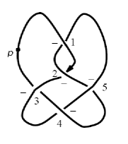
Dโ€‹(3,ฯƒ,1,5)=tโ€‹rโ€‹(Raโ€‹Rbโ€‹Rcโ€‹Rdโ€‹Raโ€‹Rdโ€‹Rฯƒโ€‹(b)โ€‹Rฯƒโ€‹(c))๐ท3๐œŽ15๐‘ก๐‘Ÿsuperscript๐‘…๐‘Žsuperscript๐‘…๐‘superscript๐‘…๐‘superscript๐‘…๐‘‘superscript๐‘…๐‘Žsuperscript๐‘…๐‘‘superscript๐‘…๐œŽ๐‘superscript๐‘…๐œŽ๐‘D(3,\sigma,1,5)\,=tr(R^{a}R^{b}R^{c}R^{d}R^{a}R^{d}R^{\sigma(b)}R^{\sigma(c)})

Refer to caption
Figure 1:

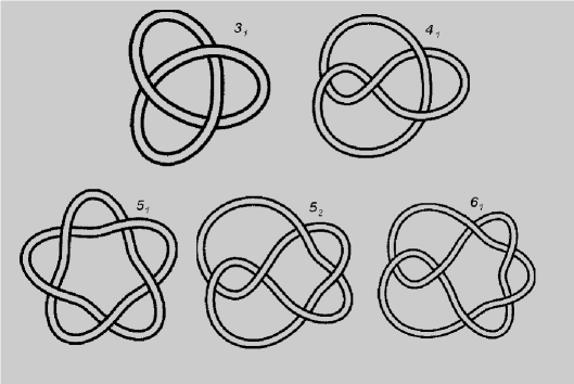
Using modern computational tools such as Maple or Mathematica and formula (3.1) one can perform computations in perturbation theory for the first several orders. In the table below some exact results of these calculus for gโ€‹lโ€‹(N)๐‘”๐‘™๐‘gl(N)-case in fundamental representation F๐นF are presented:

KnotI1FI2FI3FI4F313โ€‹N23/4โ€‹Nโ€‹(5+N2)1/12โ€‹N2โ€‹(53+N2)1192โ€‹Nโ€‹(284+363โ€‹N2+N4)4103โ€‹Nโ€‹(Nโˆ’1)โ€‹(N+1)07144โ€‹Nโ€‹(Nโˆ’1)โ€‹(N+1)โ€‹(5โ€‹N2+46)515โ€‹N25/4โ€‹Nโ€‹(9+N2)536โ€‹N2โ€‹(149+N2)5576โ€‹Nโ€‹(1712+1287โ€‹N2+N4)525โ€‹N21/4โ€‹Nโ€‹(33+17โ€‹N2)536โ€‹N2โ€‹(131+19โ€‹N2)1576โ€‹Nโ€‹(4096+10263โ€‹N2+641โ€‹N4)612โ€‹N21/2โ€‹Nโ€‹(โˆ’13+17โ€‹N2)1/9โ€‹N2โ€‹(โˆ’47+59โ€‹N2)1288N(โˆ’2394+1193N2+1393N4))\begin{array}[]{|c|c|c|c|c|}\hline\cr\textrm{Knot}&I_{1}^{F}&I_{2}^{F}&I_{3}^{F}&I_{4}^{F}\\ \hline\cr&&&&\\ 3_{1}&3\,{N}^{2}&3/4\,N(5+{N}^{2})&1/12\,{N}^{2}(53+{N}^{2})&{\frac{1}{192}}\,N(284+363\,{N}^{2}+{N}^{4})\\ &&&&\\ 4_{1}&0&3\,N(N-1)(N+1)&0&{\frac{7}{144}}\,N(N-1)(N+1)(5\,{N}^{2}+46)\\ &&&&\\ 5_{1}&5\,{N}^{2}&5/4\,N(9+{N}^{2})&{\frac{5}{36}}\,{N}^{2}(149+{N}^{2})&{\frac{5}{576}}\,N(1712+1287\,{N}^{2}+{N}^{4})\\ &&&&\\ 5_{2}&5\,{N}^{2}&1/4\,N\left(33+17\,{N}^{2}\right)&{\frac{5}{36}}\,{N}^{2}\left(131+19\,{N}^{2}\right)&{\frac{1}{576}}\,N\left(4096+10263\,{N}^{2}+641\,{N}^{4}\right)\\ &&&&\\ 6_{1}&2\,{N}^{2}&1/2\,N\left(-13+17\,{N}^{2}\right)&1/9\,{N}^{2}\left(-47+59\,{N}^{2}\right)&{\frac{1}{288}}\,N\left(-2394+1193\,{N}^{2}+1393\,{N}^{4}\right))\\ \hline\cr\end{array}

Where we have chosen the two-dimensional projections of the knots as in the fig. 2
Refer to caption
Figure 2:

In the Abelian case N=1๐‘1N=1 we get the following results:

<W^Fโ€‹(31)>=โˆ‘m=0โˆžImFโ€‹(31)โ€‹g2โ€‹m=1+3โ€‹g2+9/2โ€‹g4+9/2โ€‹g6+278โ€‹g8+8140โ€‹g10+โ€ฆ=e3โ€‹g2<W^Fโ€‹(41)>=โˆ‘m=0โˆžImโ€‹(41)โ€‹g2โ€‹m=1+0โ€‹g2+0โ€‹g4+0โ€‹g6+0โ€‹g8+0โ€‹g10+โ€ฆ=1<W^โ€‹(51)>=โˆ‘m=0โˆžImFโ€‹(51)โ€‹g2โ€‹m=1+5โ€‹g2+252โ€‹g4+1256โ€‹g6+62524โ€‹g8+62524โ€‹g10+โ€ฆ=e5โ€‹g2<W^Fโ€‹(52)>=โˆ‘m=0โˆžImFโ€‹(52)โ€‹g2โ€‹m=1+5โ€‹g2+252โ€‹g4+1256โ€‹g6+62524โ€‹g8+62524โ€‹g10+โ€ฆ=e5โ€‹g2<W^Fโ€‹(61)>=โˆ‘m=0โˆžImFโ€‹(53)โ€‹g2โ€‹m=1+2โ€‹g2+2โ€‹g4+4/3โ€‹g6+2/3โ€‹g8+415โ€‹g10+โ€ฆ=eg2expectationsubscript^๐‘Š๐นsubscript31superscriptsubscript๐‘š0superscriptsubscript๐ผ๐‘š๐นsubscript31superscript๐‘”2๐‘š13superscript๐‘”292superscript๐‘”492superscript๐‘”6278superscript๐‘”88140superscript๐‘”10โ€ฆsuperscript๐‘’3superscript๐‘”2expectationsubscript^๐‘Š๐นsubscript41superscriptsubscript๐‘š0subscript๐ผ๐‘šsubscript41superscript๐‘”2๐‘š10superscript๐‘”20superscript๐‘”40superscript๐‘”60superscript๐‘”80superscript๐‘”10โ€ฆ1expectation^๐‘Šsubscript51superscriptsubscript๐‘š0superscriptsubscript๐ผ๐‘š๐นsubscript51superscript๐‘”2๐‘š15superscript๐‘”2252superscript๐‘”41256superscript๐‘”662524superscript๐‘”862524superscript๐‘”10โ€ฆsuperscript๐‘’5superscript๐‘”2expectationsubscript^๐‘Š๐นsubscript52superscriptsubscript๐‘š0subscriptsuperscript๐ผ๐น๐‘šsubscript52superscript๐‘”2๐‘š15superscript๐‘”2252superscript๐‘”41256superscript๐‘”662524superscript๐‘”862524superscript๐‘”10โ€ฆsuperscript๐‘’5superscript๐‘”2expectationsubscript^๐‘Š๐นsubscript61superscriptsubscript๐‘š0subscriptsuperscript๐ผ๐น๐‘šsubscript53superscript๐‘”2๐‘š12superscript๐‘”22superscript๐‘”443superscript๐‘”623superscript๐‘”8415superscript๐‘”10โ€ฆsuperscript๐‘’superscript๐‘”2\begin{array}[]{l}<\hat{W}_{F}(3_{1})>\,=\sum\limits_{m=0}^{\infty}I_{m}^{F}(3_{1})\,g^{2m}=1+3\,{g}^{2}+9/2\,{g}^{4}+9/2\,{g}^{6}+{\frac{27}{8}}\,{g}^{8}+{\frac{81}{40}}\,{g}^{10}+...=e^{3\,g^{2}}\\ <\hat{W}_{F}(4_{1})>\,=\sum\limits_{m=0}^{\infty}I_{m}(4_{1})\,g^{2m}=1+0\,g^{2}+0\,g^{4}+0\,g^{6}+0\,g^{8}+0\,g^{10}+...=1\\ <\hat{W}(5_{1})>\,=\sum\limits_{m=0}^{\infty}I_{m}^{F}(5_{1})\,g^{2m}=1+5\,{g}^{2}+{\frac{25}{2}}\,{g}^{4}+{\frac{125}{6}}\,{g}^{6}+{\frac{625}{24}}\,{g}^{8}+{\frac{625}{24}}\,{g}^{10}+...=e^{5\,g^{2}}\\ <\hat{W}_{F}(5_{2})>\,=\sum\limits_{m=0}^{\infty}I^{F}_{m}(5_{2})\,g^{2m}=1+5\,{g}^{2}+{\frac{25}{2}}\,{g}^{4}+{\frac{125}{6}}\,{g}^{6}+{\frac{625}{24}}\,{g}^{8}+{\frac{625}{24}}\,{g}^{10}+...=e^{5\,g^{2}}\\ <\hat{W}_{F}(6_{1})>\,=\sum\limits_{m=0}^{\infty}I^{F}_{m}(5_{3})\,g^{2m}=1+2\,{g}^{2}+2\,{g}^{4}+4/3\,{g}^{6}+2/3\,{g}^{8}+{\frac{4}{15}}\,{g}^{10}+...=e^{g^{2}}\\ \end{array}

We see that in full agreement with (13) the vevs of the Wilson loops in this cases are just products of simple exponent operators over intersection points. In the first non-abelian case N=2๐‘2N=2 we get:

<W^Fโ€‹(31)>=โˆ‘m=0โˆžImFโ€‹(31)โ€‹g2โ€‹m=2+12โ€‹g2+272โ€‹g4+19โ€‹g6+734โ€‹g8+27920โ€‹g10+โ€ฆ=?<W^Fโ€‹(41)>=โˆ‘m=0โˆžImFโ€‹(41)โ€‹g2โ€‹m=2+18โ€‹g4+774โ€‹g8+โ€ฆ=?<W^Fโ€‹(51)>=โˆ‘m=0โˆžImFโ€‹(51)โ€‹g2โ€‹m=2+20โ€‹g2+652โ€‹g4+85โ€‹g6+9558โ€‹g8+8716โ€‹g10+โ€ฆ=?<W^Fโ€‹(52)>=โˆ‘m=0โˆžImFโ€‹(52)โ€‹g2โ€‹m=2+20โ€‹g2+1012โ€‹g4+115โ€‹g6+15398โ€‹g8+15856โ€‹g10+โ€ฆ=?<W^Fโ€‹(61)>=โˆ‘m=0โˆžImFโ€‹(53)โ€‹g2โ€‹m=2+8โ€‹g2+55โ€‹g4+84โ€‹g6+411124โ€‹g8+291215โ€‹g10+โ€ฆ=?expectationsubscript^๐‘Š๐นsubscript31superscriptsubscript๐‘š0superscriptsubscript๐ผ๐‘š๐นsubscript31superscript๐‘”2๐‘š212superscript๐‘”2272superscript๐‘”419superscript๐‘”6734superscript๐‘”827920superscript๐‘”10โ€ฆ?expectationsubscript^๐‘Š๐นsubscript41superscriptsubscript๐‘š0superscriptsubscript๐ผ๐‘š๐นsubscript41superscript๐‘”2๐‘š218superscript๐‘”4774superscript๐‘”8โ€ฆ?expectationsubscript^๐‘Š๐นsubscript51superscriptsubscript๐‘š0superscriptsubscript๐ผ๐‘š๐นsubscript51superscript๐‘”2๐‘š220superscript๐‘”2652superscript๐‘”485superscript๐‘”69558superscript๐‘”88716superscript๐‘”10โ€ฆ?expectationsubscript^๐‘Š๐นsubscript52superscriptsubscript๐‘š0superscriptsubscript๐ผ๐‘š๐นsubscript52superscript๐‘”2๐‘š220superscript๐‘”21012superscript๐‘”4115superscript๐‘”615398superscript๐‘”815856superscript๐‘”10โ€ฆ?expectationsubscript^๐‘Š๐นsubscript61superscriptsubscript๐‘š0superscriptsubscript๐ผ๐‘š๐นsubscript53superscript๐‘”2๐‘š28superscript๐‘”255superscript๐‘”484superscript๐‘”6411124superscript๐‘”8291215superscript๐‘”10โ€ฆ?\begin{array}[]{l}<\hat{W}_{F}(3_{1})>\,=\sum\limits_{m=0}^{\infty}I_{m}^{F}(3_{1})\,g^{2m}=2+12\,{g}^{2}+{\frac{27}{2}}\,{g}^{4}+19\,{g}^{6}+{\frac{73}{4}}\,{g}^{8}+{\frac{279}{20}}\,{g}^{10}+...=\,?\\ <\hat{W}_{F}(4_{1})>\,=\sum\limits_{m=0}^{\infty}I_{m}^{F}(4_{1})\,g^{2m}=2+18\,{g}^{4}+{\frac{77}{4}}\,{g}^{8}+...=\,?\\ <\hat{W}_{F}(5_{1})>=\sum\limits_{m=0}^{\infty}I_{m}^{F}(5_{1})\,g^{2m}=2+20\,{g}^{2}+{\frac{65}{2}}\,{g}^{4}+85\,{g}^{6}+{\frac{955}{8}}\,{g}^{8}+{\frac{871}{6}}\,{g}^{10}+...=\,?\\ <\hat{W}_{F}(5_{2})>\,=\sum\limits_{m=0}^{\infty}I_{m}^{F}(5_{2})\,g^{2m}=2+20\,{g}^{2}+{\frac{101}{2}}\,{g}^{4}+115\,{g}^{6}+{\frac{1539}{8}}\,{g}^{8}+{\frac{1585}{6}}\,{g}^{10}+...=\,?\\ <\hat{W}_{F}(6_{1})>\,=\sum\limits_{m=0}^{\infty}I_{m}^{F}(5_{3})\,g^{2m}=2+8\,{g}^{2}+55\,{g}^{4}+84\,{g}^{6}+{\frac{4111}{24}}\,{g}^{8}+{\frac{2912}{15}}\,{g}^{10}\par+...=\,?\\ \end{array}

In this case it is difficult to find any regularity in the coefficients of the expansions and sum them to the exact expressions of vevs for kernels of associated Wilson loops operators. It indicates that the answer for these vevs in non-abelian case has much more complicated structure. In section 4 we present the example of such vev for the simplest trefoil knot 31subscript313_{1} in the case N=2๐‘2N=2.

3.2 Two-Component Links

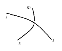
In order to derive the notion of intersection point operator we need to find a contribution to vev of Wilson loop coming from a single two-dimensional intersection point as in fig.3. For our analysis it is much more convenient to assume that the pathes iโ€‹j๐‘–๐‘—i\,j and kโ€‹m๐‘˜๐‘šk\,m belong to different contours.

Refer to caption
Figure 3:

In this connection let us temporary proceed to the consideration of two-component links. More precisely, we are interested in the following quantity:

IR1โ€‹R2โ€‹(c1,c2)=<W^R1(c1),W^R2(c2)><W^R1โ€‹(c1)>โ€‹<W^R2โ€‹(c2)>=โˆ‘k=0โˆžIkR1โ€‹R2โ€‹(c1,c2)โ€‹g2โ€‹k=1+โˆ‘k=1โˆžIkR1โ€‹R2โ€‹(c1,c2)โ€‹g2โ€‹kI^{R_{1}\,R_{2}}(c_{1},c_{2})=\dfrac{<\hat{W}_{R_{1}}(c_{1}),\,\hat{W}_{R_{2}}(c_{2})>}{<\hat{W}_{R_{1}}(c_{1})><\hat{W}_{R_{2}}(c_{2})>}=\sum\limits_{k=0}^{\infty}I_{k}^{R_{1}\,R_{2}}(c_{1},c_{2})g^{2\,k}=1+\sum\limits_{k=1}^{\infty}I_{k}^{R_{1}\,R_{2}}(c_{1},c_{2})g^{2\,k} (15)

where c1subscript๐‘1c_{1} and c2subscript๐‘2c_{2} are two contours in โ„3superscriptโ„3\mathbb{R}^{3} and WRiโ€‹(ci)subscript๐‘Šsubscript๐‘…๐‘–subscript๐‘๐‘–W_{R_{i}}(c_{i}) are associated Wilson lines operators in representation Risubscript๐‘…๐‘–R_{i} of the gauge group:

WRiโ€‹(ci)=tโ€‹rโ€‹Pโ€‹expโก(gโ€‹โˆฎciAฮผโ€‹๐‘‘xฮผ)subscript๐‘Šsubscript๐‘…๐‘–subscript๐‘๐‘–๐‘ก๐‘Ÿ๐‘ƒ๐‘”subscriptcontour-integralsubscript๐‘๐‘–subscript๐ด๐œ‡differential-dsuperscript๐‘ฅ๐œ‡W_{R_{i}}(c_{i})=trP\exp\left(g\oint\limits_{c_{i}}A_{\mu}\,dx^{\mu}\right) (16)

In (15) we divided vev <W^R1(c1),W^R2(c2)><\hat{W}_{R_{1}}(c_{1}),\,\hat{W}_{R_{2}}(c_{2})> by the product of vevs <W^R1โ€‹(c1)>โ€‹<W^R2โ€‹(c2)>expectationsubscript^๐‘Šsubscript๐‘…1subscript๐‘1expectationsubscript^๐‘Šsubscript๐‘…2subscript๐‘2<\hat{W}_{R_{1}}(c_{1})><\hat{W}_{R_{2}}(c_{2})>, which means that in perturbation series expansion we will only take into account the terms with different ends of the propagators attached to the different contours, in other words, we do not take into consideration the self-intersection points of the contours c1subscript๐‘1c_{1} and c2subscript๐‘2c_{2}.

3.3 I1R1โ€‹R2โ€‹(c1,c2)superscriptsubscript๐ผ1subscript๐‘…1subscript๐‘…2subscript๐‘1subscript๐‘2I_{1}^{R_{1}\,R_{2}}(c_{1},c_{2}) case

In the order g2superscript๐‘”2g^{2} we have the following integral:

I1R1โ€‹R2โ€‹(c1,c2)=g2โ€‹tโ€‹rโ€‹(R1a)โ€‹tโ€‹rโ€‹(R2b)โ€‹โˆฎc1๐‘‘xฮผโ€‹โˆฎc2๐‘‘yฮฝ<Aฮผaโ€‹(x),Aฮฝbโ€‹(y)>=0formulae-sequencesuperscriptsubscript๐ผ1subscript๐‘…1subscript๐‘…2subscript๐‘1subscript๐‘2superscript๐‘”2๐‘ก๐‘Ÿsuperscriptsubscript๐‘…1๐‘Ž๐‘ก๐‘Ÿsuperscriptsubscript๐‘…2๐‘subscriptcontour-integralsubscript๐‘1differential-dsuperscript๐‘ฅ๐œ‡subscriptcontour-integralsubscript๐‘2differential-dsuperscript๐‘ฆ๐œˆsuperscriptsubscript๐ด๐œ‡๐‘Ž๐‘ฅsuperscriptsubscript๐ด๐œˆ๐‘๐‘ฆ0\displaystyle I_{1}^{R_{1}\,R_{2}}(c_{1},\,c_{2})=g^{2}\,tr(R_{1}^{a})\,tr(R_{2}^{b})\,\oint\limits_{c_{1}}\,dx^{\mu}\oint\limits_{c_{2}}\,dy^{\nu}<A_{\mu}^{a}(x),\,A_{\nu}^{b}(y)>=0

3.4 I2R1โ€‹R2โ€‹(c1,c2)superscriptsubscript๐ผ2subscript๐‘…1subscript๐‘…2subscript๐‘1subscript๐‘2I_{2}^{R_{1}\,R_{2}}(c_{1},c_{2}) case

In the order g4superscript๐‘”4g^{4} we have two contributions:

I2R1โ€‹R2โ€‹(c1,c2)=M1+M2superscriptsubscript๐ผ2subscript๐‘…1subscript๐‘…2subscript๐‘1subscript๐‘2subscript๐‘€1subscript๐‘€2I_{2}^{R_{1}\,R_{2}}(c_{1},c_{2})=M_{1}+M_{2} (17)

where

M1=tr(R1a1R1a2)tr(R2b1R2b2)โˆฎc1dx1ฮผ1โˆซc1x1dx2ฮผ2โˆฎc2dy1ฮฝ1โˆซc2y1dy2ฮฝ2<Aฮผ1a1(x1),Aฮฝ1b1(y1)><Aฮผ2a2(x2),Aฮฝ2b2(y2)>\displaystyle M_{1}=tr(R_{1}^{a_{1}}R_{1}^{a_{2}})\,tr(R_{2}^{b_{1}}R_{2}^{b_{2}})\oint\limits_{c_{1}}dx_{1}^{\mu_{1}}\int\limits_{c_{1}}^{x_{1}}dx_{2}^{\mu_{2}}\oint\limits_{c_{2}}dy_{1}^{\nu_{1}}\int\limits_{c_{2}}^{y_{1}}dy_{2}^{\nu_{2}}<A_{\mu_{1}}^{a_{1}}(x_{1}),\,A_{\nu_{1}}^{b_{1}}(y_{1})>\,<A_{\mu_{2}}^{a_{2}}(x_{2}),\,A_{\nu_{2}}^{b_{2}}(y_{2})> (18)
M2=tr(R1a1R1a2)tr(R2b1R2b2)โˆฎc1dx1ฮผ1โˆซc1x1dx2ฮผ2โˆฎc2dy1ฮฝ1โˆซc2y1dy2ฮฝ2<Aฮผ1a1(x1),Aฮฝ2b2(y2)><Aฮผ2a2(x2),Aฮฝ1b1(y1)>\displaystyle M_{2}=tr(R_{1}^{a_{1}}R_{1}^{a_{2}})\,tr(R_{2}^{b_{1}}R_{2}^{b_{2}})\oint\limits_{c_{1}}dx_{1}^{\mu_{1}}\int\limits_{c_{1}}^{x_{1}}dx_{2}^{\mu_{2}}\oint\limits_{c_{2}}dy_{1}^{\nu_{1}}\int\limits_{c_{2}}^{y_{1}}dy_{2}^{\nu_{2}}<A_{\mu_{1}}^{a_{1}}(x_{1}),\,A_{\nu_{2}}^{b_{2}}(y_{2})>\,<A_{\mu_{2}}^{a_{2}}(x_{2}),\,A_{\nu_{1}}^{b_{1}}(y_{1})> (19)

Introducing the parameterizations t๐‘กt and s๐‘ s for contours c1subscript๐‘1c_{1} and c2subscript๐‘2c_{2} respectively we get:

Gโ€‹(t,s)=ฯตฮผโ€‹ฮฝโ€‹dโ€‹xฮผdโ€‹tโ€‹(t)โ€‹dโ€‹yฮฝdโ€‹sโ€‹(s)โ€‹ฮดโ€‹(x1โ€‹(t)โˆ’y1โ€‹(s))โ€‹ฮดโ€‹(x2โ€‹(t)โˆ’y2โ€‹(s))โ€‹12โ€‹signโ€‹(x0โ€‹(t)โˆ’y0โ€‹(s))=โˆ‘kฯตkโ€‹ฮดโ€‹(tโˆ’tk)โ€‹ฮดโ€‹(sโˆ’sk)๐บ๐‘ก๐‘ subscriptitalic-ฯต๐œ‡๐œˆ๐‘‘superscript๐‘ฅ๐œ‡๐‘‘๐‘ก๐‘ก๐‘‘superscript๐‘ฆ๐œˆ๐‘‘๐‘ ๐‘ ๐›ฟsubscript๐‘ฅ1๐‘กsubscript๐‘ฆ1๐‘ ๐›ฟsubscript๐‘ฅ2๐‘กsubscript๐‘ฆ2๐‘ 12signsubscript๐‘ฅ0๐‘กsubscript๐‘ฆ0๐‘ subscript๐‘˜subscriptitalic-ฯต๐‘˜๐›ฟ๐‘กsubscript๐‘ก๐‘˜๐›ฟ๐‘ subscript๐‘ ๐‘˜G(t,s)=\epsilon_{\mu\,\nu}\,\dfrac{dx^{\mu}}{dt}(t)\,\dfrac{dy^{\nu}}{ds}(s)\,\delta(x_{1}(t)-y_{1}(s))\,\delta(x_{2}(t)-y_{2}(s))\,\dfrac{1}{2}\textrm{sign}(x_{0}(t)-y_{0}(s))=\sum\limits_{k}\epsilon_{k}\delta(t-t_{k})\delta(s-s_{k})

Here ฯตk=ยฑ1subscriptitalic-ฯต๐‘˜plus-or-minus1\epsilon_{k}=\pm 1 and sum runs over the intersection points of two contours lying in the plane (x1,x2)subscript๐‘ฅ1subscript๐‘ฅ2(x_{1},x_{2}) which are the projections of three dimensional contours on the plane. Using this notation we can rewrite the integrals for M1subscript๐‘€1M_{1} and M2subscript๐‘€2M_{2} in the form:

M1=tโ€‹rโ€‹(R1a1โ€‹R1a2)โ€‹tโ€‹rโ€‹(R2a1โ€‹R2a2)โ€‹โˆซ01๐‘‘t1โ€‹โˆซ0t1๐‘‘t2โ€‹โˆซ01๐‘‘s1โ€‹โˆซ0s1๐‘‘s2โ€‹Gโ€‹(t1,s1)โ€‹Gโ€‹(t2,s2)subscript๐‘€1๐‘ก๐‘Ÿsuperscriptsubscript๐‘…1subscript๐‘Ž1superscriptsubscript๐‘…1subscript๐‘Ž2๐‘ก๐‘Ÿsuperscriptsubscript๐‘…2subscript๐‘Ž1superscriptsubscript๐‘…2subscript๐‘Ž2superscriptsubscript01differential-dsubscript๐‘ก1superscriptsubscript0subscript๐‘ก1differential-dsubscript๐‘ก2superscriptsubscript01differential-dsubscript๐‘ 1superscriptsubscript0subscript๐‘ 1differential-dsubscript๐‘ 2๐บsubscript๐‘ก1subscript๐‘ 1๐บsubscript๐‘ก2subscript๐‘ 2\displaystyle M_{1}=tr(R_{1}^{a_{1}}R_{1}^{a_{2}})\,tr(R_{2}^{a_{1}}R_{2}^{a_{2}})\,\int\limits_{0}^{1}dt_{1}\int\limits_{0}^{t_{1}}dt_{2}\,\int\limits_{0}^{1}ds_{1}\int\limits_{0}^{s_{1}}ds_{2}\,G(t_{1},\,s_{1})\,G(t_{2},\,s_{2}) (20)
M2=tโ€‹rโ€‹(R1a1โ€‹R1a2)โ€‹tโ€‹rโ€‹(R2a2โ€‹R2a1)โ€‹โˆซ01๐‘‘t1โ€‹โˆซ0t1๐‘‘t2โ€‹โˆซ01๐‘‘s1โ€‹โˆซ0s1๐‘‘s2โ€‹Gโ€‹(t1,s2)โ€‹Gโ€‹(t2,s1)subscript๐‘€2๐‘ก๐‘Ÿsuperscriptsubscript๐‘…1subscript๐‘Ž1superscriptsubscript๐‘…1subscript๐‘Ž2๐‘ก๐‘Ÿsuperscriptsubscript๐‘…2subscript๐‘Ž2superscriptsubscript๐‘…2subscript๐‘Ž1superscriptsubscript01differential-dsubscript๐‘ก1superscriptsubscript0subscript๐‘ก1differential-dsubscript๐‘ก2superscriptsubscript01differential-dsubscript๐‘ 1superscriptsubscript0subscript๐‘ 1differential-dsubscript๐‘ 2๐บsubscript๐‘ก1subscript๐‘ 2๐บsubscript๐‘ก2subscript๐‘ 1\displaystyle M_{2}=tr(R_{1}^{a_{1}}R_{1}^{a_{2}})\,tr(R_{2}^{a_{2}}R_{2}^{a_{1}})\,\int\limits_{0}^{1}dt_{1}\int\limits_{0}^{t_{1}}dt_{2}\,\int\limits_{0}^{1}ds_{1}\int\limits_{0}^{s_{1}}ds_{2}\,G(t_{1},\,s_{2})\,G(t_{2},\,s_{1}) (21)

and using the following fact:

โˆซ01๐‘‘t1โ€‹โˆซ0t1๐‘‘t2โ€‹โˆซ01๐‘‘s1โ€‹โˆซ0s1๐‘‘s2=โˆซ01๐‘‘t1โ€‹โˆซ01๐‘‘t2โ€‹โˆซ01๐‘‘s1โ€‹โˆซ01๐‘‘s2โ€‹ฮธโ€‹(t1โˆ’t2)โ€‹ฮธโ€‹(s1โˆ’s2)superscriptsubscript01differential-dsubscript๐‘ก1superscriptsubscript0subscript๐‘ก1differential-dsubscript๐‘ก2superscriptsubscript01differential-dsubscript๐‘ 1superscriptsubscript0subscript๐‘ 1differential-dsubscript๐‘ 2superscriptsubscript01differential-dsubscript๐‘ก1superscriptsubscript01differential-dsubscript๐‘ก2superscriptsubscript01differential-dsubscript๐‘ 1superscriptsubscript01differential-dsubscript๐‘ 2๐œƒsubscript๐‘ก1subscript๐‘ก2๐œƒsubscript๐‘ 1subscript๐‘ 2\int\limits_{0}^{1}dt_{1}\int\limits_{0}^{t_{1}}dt_{2}\,\int\limits_{0}^{1}ds_{1}\int\limits_{0}^{s_{1}}ds_{2}=\int\limits_{0}^{1}dt_{1}\int\limits_{0}^{1}dt_{2}\,\int\limits_{0}^{1}ds_{1}\int\limits_{0}^{1}ds_{2}\,\theta(t_{1}-t_{2})\theta(s_{1}-s_{2}) (22)

we have:

M1=tโ€‹rโ€‹(R1a1โ€‹R1a2)โ€‹tโ€‹rโ€‹(R2a1โ€‹R2a2)โ€‹โˆ‘k1โ€‹k2ฯตk1โ€‹ฯตk2โ€‹ฮธโ€‹(tk1โˆ’tk2)โ€‹ฮธโ€‹(sk1โˆ’sk2)subscript๐‘€1๐‘ก๐‘Ÿsuperscriptsubscript๐‘…1subscript๐‘Ž1superscriptsubscript๐‘…1subscript๐‘Ž2๐‘ก๐‘Ÿsuperscriptsubscript๐‘…2subscript๐‘Ž1superscriptsubscript๐‘…2subscript๐‘Ž2subscriptsubscript๐‘˜1subscript๐‘˜2subscriptitalic-ฯตsubscript๐‘˜1subscriptitalic-ฯตsubscript๐‘˜2๐œƒsubscript๐‘กsubscript๐‘˜1subscript๐‘กsubscript๐‘˜2๐œƒsubscript๐‘ subscript๐‘˜1subscript๐‘ subscript๐‘˜2\displaystyle M_{1}=tr(R_{1}^{a_{1}}R_{1}^{a_{2}})\,tr(R_{2}^{a_{1}}R_{2}^{a_{2}})\,\sum_{k_{1}\,k_{2}}\,\epsilon_{k_{1}}\epsilon_{k_{2}}\,\theta(t_{k_{1}}-t_{k_{2}})\,\theta(s_{k_{1}}-s_{k_{2}})
(23)
M2=tโ€‹rโ€‹(R1a1โ€‹R1a2)โ€‹tโ€‹rโ€‹(R2a2โ€‹R2a1)โ€‹โˆ‘k1โ€‹k2ฯตk1โ€‹ฯตk2โ€‹ฮธโ€‹(tk1โˆ’tk2)โ€‹ฮธโ€‹(sk2โˆ’sk1)subscript๐‘€2๐‘ก๐‘Ÿsuperscriptsubscript๐‘…1subscript๐‘Ž1superscriptsubscript๐‘…1subscript๐‘Ž2๐‘ก๐‘Ÿsuperscriptsubscript๐‘…2subscript๐‘Ž2superscriptsubscript๐‘…2subscript๐‘Ž1subscriptsubscript๐‘˜1subscript๐‘˜2subscriptitalic-ฯตsubscript๐‘˜1subscriptitalic-ฯตsubscript๐‘˜2๐œƒsubscript๐‘กsubscript๐‘˜1subscript๐‘กsubscript๐‘˜2๐œƒsubscript๐‘ subscript๐‘˜2subscript๐‘ subscript๐‘˜1\displaystyle M_{2}=tr(R_{1}^{a_{1}}R_{1}^{a_{2}})\,tr(R_{2}^{a_{2}}R_{2}^{a_{1}})\,\sum_{k_{1}\,k_{2}}\,\epsilon_{k_{1}}\epsilon_{k_{2}}\,\theta(t_{k_{1}}-t_{k_{2}})\,\theta(s_{k_{2}}-s_{k_{1}})

and finally we arrive to the following expression:

I2R1โ€‹R2โ€‹(c1,c2)=M1+M2=โˆ‘ฯƒโˆˆS2tโ€‹rโ€‹(R1a1โ€‹R1a2)โ€‹tโ€‹rโ€‹(R2aฯƒโ€‹(1)โ€‹R2aฯƒโ€‹(2))โ€‹โˆ‘k1โ€‹k2ฯตk1โ€‹ฯตk2โ€‹ฮธโ€‹(tk1โˆ’tk2)โ€‹ฮธโ€‹(skฯƒโ€‹(1)โˆ’skฯƒโ€‹(2))superscriptsubscript๐ผ2subscript๐‘…1subscript๐‘…2subscript๐‘1subscript๐‘2subscript๐‘€1subscript๐‘€2subscript๐œŽsubscript๐‘†2๐‘ก๐‘Ÿsuperscriptsubscript๐‘…1subscript๐‘Ž1superscriptsubscript๐‘…1subscript๐‘Ž2๐‘ก๐‘Ÿsuperscriptsubscript๐‘…2subscript๐‘Ž๐œŽ1superscriptsubscript๐‘…2subscript๐‘Ž๐œŽ2subscriptsubscript๐‘˜1subscript๐‘˜2subscriptitalic-ฯตsubscript๐‘˜1subscriptitalic-ฯตsubscript๐‘˜2๐œƒsubscript๐‘กsubscript๐‘˜1subscript๐‘กsubscript๐‘˜2๐œƒsubscript๐‘ subscript๐‘˜๐œŽ1subscript๐‘ subscript๐‘˜๐œŽ2I_{2}^{R_{1}\,R_{2}}(c_{1},c_{2})=M_{1}+M_{2}=\sum_{\sigma\in S_{2}}tr(R_{1}^{a_{1}}R_{1}^{a_{2}})\,tr(R_{2}^{a_{\sigma(1)}}R_{2}^{a_{\sigma(2)}})\,\sum_{k_{1}\,k_{2}}\,\epsilon_{k_{1}}\epsilon_{k_{2}}\,\theta(t_{k_{1}}-t_{k_{2}})\,\theta(s_{k_{\sigma(1)}}-s_{k_{\sigma(2)}}) (24)

where S2subscript๐‘†2S_{2} is the permutation group of two elements.

3.5 ImR1โ€‹R2โ€‹(c1โ€‹c2)superscriptsubscript๐ผ๐‘šsubscript๐‘…1subscript๐‘…2subscript๐‘1subscript๐‘2I_{m}^{R_{1}\,R_{2}}(c_{1}\,c_{2}) Case

The last formula (24) has obvious straightforward generalization for ImR1โ€‹R2โ€‹(c1โ€‹c2)superscriptsubscript๐ผ๐‘šsubscript๐‘…1subscript๐‘…2subscript๐‘1subscript๐‘2I_{m}^{R_{1}\,R_{2}}(c_{1}\,c_{2}):

ImR1โ€‹R2โ€‹(c1โ€‹c2)=โˆ‘ฯƒโˆˆSmMฯƒsuperscriptsubscript๐ผ๐‘šsubscript๐‘…1subscript๐‘…2subscript๐‘1subscript๐‘2subscript๐œŽsubscript๐‘†๐‘šsubscript๐‘€๐œŽI_{m}^{R_{1}\,R_{2}}(c_{1}\,c_{2})=\sum\limits_{\sigma\in\,S_{m}}M_{\sigma} (25)

where Smsubscript๐‘†๐‘šS_{m} is the permutation group for a set with m๐‘šm elements.

Mฯƒ=tโ€‹rโ€‹(R1a1โ€‹โ€ฆโ€‹R1am)โ€‹tโ€‹rโ€‹(R2aฯƒโ€‹(1)โ€‹โ€ฆโ€‹R2aฯƒโ€‹(m))โ€‹โˆ‘k1โ€‹k2โ€‹โ€ฆโ€‹kmฯตk1โ€‹ฯตk2โ€‹โ€ฆโ€‹ฯตkmโ€‹(โˆi=1mโˆ’1ฮธโ€‹(tkiโˆ’tki+1))โ€‹(โˆj=1mโˆ’1ฮธโ€‹(skฯƒโ€‹(j)โˆ’skฯƒโ€‹(j+1)))subscript๐‘€๐œŽ๐‘ก๐‘Ÿsuperscriptsubscript๐‘…1subscript๐‘Ž1โ€ฆsuperscriptsubscript๐‘…1subscript๐‘Ž๐‘š๐‘ก๐‘Ÿsuperscriptsubscript๐‘…2subscript๐‘Ž๐œŽ1โ€ฆsuperscriptsubscript๐‘…2subscript๐‘Ž๐œŽ๐‘šsubscriptsubscript๐‘˜1subscript๐‘˜2โ€ฆsubscript๐‘˜๐‘šsubscriptitalic-ฯตsubscript๐‘˜1subscriptitalic-ฯตsubscript๐‘˜2โ€ฆsubscriptitalic-ฯตsubscript๐‘˜๐‘šsuperscriptsubscriptproduct๐‘–1๐‘š1๐œƒsubscript๐‘กsubscript๐‘˜๐‘–subscript๐‘กsubscript๐‘˜๐‘–1superscriptsubscriptproduct๐‘—1๐‘š1๐œƒsubscript๐‘ subscript๐‘˜๐œŽ๐‘—subscript๐‘ subscript๐‘˜๐œŽ๐‘—1M_{\sigma}=tr(R_{1}^{a_{1}}...R_{1}^{a_{m}})tr(R_{2}^{a_{\sigma(1)}}...R_{2}^{a_{\sigma(m)}})\sum\limits_{k_{1}\,k_{2}...k_{m}}\epsilon_{k_{1}}\epsilon_{k_{2}}...\epsilon_{k_{m}}\left(\prod\limits_{i=1}^{m-1}\theta(t_{k_{i}}-t_{k_{i+1}})\right)\,\left(\prod\limits_{j=1}^{m-1}\theta\left(s_{k_{\sigma(j)}}-s_{k_{\sigma(j+1)}}\right)\right) (26)

Let us note that in the Abelian case Mฯƒsubscript๐‘€๐œŽM_{\sigma} does not contain non-commuting lie-algebra structures and the sum of Mฯƒsubscript๐‘€๐œŽM_{\sigma} is expressed through the linking number of two contours:

โˆ‘ฯƒโˆˆSmMฯƒ=โˆ‘ฯƒโˆˆSm(โˆ‘k1โ€‹k2โ€‹โ€ฆโ€‹kmฯตk1โ€‹ฯตk2โ€‹โ€ฆโ€‹ฯตkmโ€‹(โˆi=1mโˆ’1ฮธโ€‹(tkiโˆ’tki+1))โ€‹(โˆj=1mโˆ’1ฮธโ€‹(skฯƒโ€‹(j)โˆ’skฯƒโ€‹(j+1))))=L12mm!subscript๐œŽsubscript๐‘†๐‘šsubscript๐‘€๐œŽsubscript๐œŽsubscript๐‘†๐‘šsubscriptsubscript๐‘˜1subscript๐‘˜2โ€ฆsubscript๐‘˜๐‘šsubscriptitalic-ฯตsubscript๐‘˜1subscriptitalic-ฯตsubscript๐‘˜2โ€ฆsubscriptitalic-ฯตsubscript๐‘˜๐‘šsuperscriptsubscriptproduct๐‘–1๐‘š1๐œƒsubscript๐‘กsubscript๐‘˜๐‘–subscript๐‘กsubscript๐‘˜๐‘–1superscriptsubscriptproduct๐‘—1๐‘š1๐œƒsubscript๐‘ subscript๐‘˜๐œŽ๐‘—subscript๐‘ subscript๐‘˜๐œŽ๐‘—1superscriptsubscript๐ฟ12๐‘š๐‘š\sum_{\sigma\in\,S_{m}}\,M_{\sigma}\,=\sum_{\sigma\in\,S_{m}}\left(\sum\limits_{k_{1}\,k_{2}...k_{m}}\epsilon_{k_{1}}\epsilon_{k_{2}}...\epsilon_{k_{m}}\left(\prod\limits_{i\,=1}^{m-1}\theta(t_{k_{i}}-t_{k_{i+1}})\right)\,\left(\prod\limits_{j\,=1}^{m-1}\theta\left(s_{k_{\sigma(j)}}-s_{k_{\sigma(j+1)}}\right)\right)\right)=\dfrac{L_{12}^{m}}{m!} (27)

where the quantity L12subscript๐ฟ12L_{12} is just a sum of crossing sings over two dimensional intersection points:

L12=โˆ‘kฯตksubscript๐ฟ12subscript๐‘˜subscriptitalic-ฯต๐‘˜L_{12}=\sum_{k}\epsilon_{k}

The definition of L12subscript๐ฟ12L_{12} coincides precisely with definition of linking number of two knots. The linking number of two two-component link known to be the topological invariant of the link, and we arrive to the following result: in abelian case the vev (15) is just the exponent of linking number of the link:

Iโ€‹(c1,c2)=โˆ‘m=0โˆžg2โ€‹kโ€‹L12mm!=expโก(g2โ€‹L12)๐ผsubscript๐‘1subscript๐‘2superscriptsubscript๐‘š0superscript๐‘”2๐‘˜superscriptsubscript๐ฟ12๐‘š๐‘šsuperscript๐‘”2subscript๐ฟ12I(c_{1},c_{2})=\sum_{m=0}^{\infty}g^{2k}\,\dfrac{L_{12}^{m}}{m!}=\exp(g^{2}\,L_{12})

4 The intersection point operator method

4.1 The intersection point operator

Using the following property of the tensor product of operators:

tโ€‹rโ€‹(R1a1โ€‹R1a2โ€‹โ€ฆโ€‹R1am)โ€‹tโ€‹rโ€‹(R2aฯƒโ€‹(1)โ€‹R2aฯƒโ€‹(2)โ€‹โ€ฆโ€‹R2aฯƒโ€‹(m))=tโ€‹rโ€‹(R1a1โ€‹R1a2โ€‹โ€ฆโ€‹R1amโŠ—R2aฯƒโ€‹(1)โ€‹R2aฯƒโ€‹(2)โ€‹โ€ฆโ€‹R2aฯƒโ€‹(m))๐‘ก๐‘Ÿsuperscriptsubscript๐‘…1subscript๐‘Ž1superscriptsubscript๐‘…1subscript๐‘Ž2โ€ฆsuperscriptsubscript๐‘…1subscript๐‘Ž๐‘š๐‘ก๐‘Ÿsuperscriptsubscript๐‘…2subscript๐‘Ž๐œŽ1superscriptsubscript๐‘…2subscript๐‘Ž๐œŽ2โ€ฆsuperscriptsubscript๐‘…2subscript๐‘Ž๐œŽ๐‘š๐‘ก๐‘Ÿtensor-productsuperscriptsubscript๐‘…1subscript๐‘Ž1superscriptsubscript๐‘…1subscript๐‘Ž2โ€ฆsuperscriptsubscript๐‘…1subscript๐‘Ž๐‘šsuperscriptsubscript๐‘…2subscript๐‘Ž๐œŽ1superscriptsubscript๐‘…2subscript๐‘Ž๐œŽ2โ€ฆsuperscriptsubscript๐‘…2subscript๐‘Ž๐œŽ๐‘štr(R_{1}^{a_{1}}R_{1}^{a_{2}}...R_{1}^{a_{m}})tr(R_{2}^{a_{\sigma(1)}}R_{2}^{a_{\sigma(2)}}...R_{2}^{a_{\sigma(m)}})=tr(R_{1}^{a_{1}}R_{1}^{a_{2}}...R_{1}^{a_{m}}\otimes R_{2}^{a_{\sigma(1)}}R_{2}^{a_{\sigma(2)}}...R_{2}^{a_{\sigma(m)}})

we can rewrite expression for ImR1โ€‹R2โ€‹(c1,c2)superscriptsubscript๐ผ๐‘šsubscript๐‘…1subscript๐‘…2subscript๐‘1subscript๐‘2I_{m}^{R_{1}\,R_{2}}(c_{1},c_{2}) in the form:

Mฯƒ=tโ€‹rโ€‹(M^ฯƒ)subscript๐‘€๐œŽ๐‘ก๐‘Ÿsubscript^๐‘€๐œŽM_{\sigma}=tr({\hat{M}}_{\sigma})
M^ฯƒ=R1a1โ€‹โ€ฆโ€‹R1amโŠ—R2aฯƒโ€‹(1)โ€‹โ€ฆโ€‹R2aฯƒโ€‹(m)โ€‹โˆ‘k1โ€‹k2โ€‹โ€ฆโ€‹kmฯตk1โ€‹ฯตk2โ€‹โ€ฆโ€‹ฯตkmโ€‹(โˆi=1mโˆ’1ฮธโ€‹(tkiโˆ’tki+1))โ€‹(โˆj=1mโˆ’1ฮธโ€‹(skฯƒโ€‹(j)โˆ’skฯƒโ€‹(j+1)))subscript^๐‘€๐œŽtensor-productsuperscriptsubscript๐‘…1subscript๐‘Ž1โ€ฆsuperscriptsubscript๐‘…1subscript๐‘Ž๐‘šsuperscriptsubscript๐‘…2subscript๐‘Ž๐œŽ1โ€ฆsuperscriptsubscript๐‘…2subscript๐‘Ž๐œŽ๐‘šsubscriptsubscript๐‘˜1subscript๐‘˜2โ€ฆsubscript๐‘˜๐‘šsubscriptitalic-ฯตsubscript๐‘˜1subscriptitalic-ฯตsubscript๐‘˜2โ€ฆsubscriptitalic-ฯตsubscript๐‘˜๐‘šsuperscriptsubscriptproduct๐‘–1๐‘š1๐œƒsubscript๐‘กsubscript๐‘˜๐‘–subscript๐‘กsubscript๐‘˜๐‘–1superscriptsubscriptproduct๐‘—1๐‘š1๐œƒsubscript๐‘ subscript๐‘˜๐œŽ๐‘—subscript๐‘ subscript๐‘˜๐œŽ๐‘—1{\hat{M}}_{\sigma}=R_{1}^{a_{1}}...R_{1}^{a_{m}}\otimes R_{2}^{a_{\sigma(1)}}...R_{2}^{a_{\sigma(m)}}\sum\limits_{k_{1}\,k_{2}...k_{m}}\epsilon_{k_{1}}\epsilon_{k_{2}}...\epsilon_{k_{m}}\left(\prod\limits_{i=1}^{m-1}\theta(t_{k_{i}}-t_{k_{i+1}})\right)\,\left(\prod\limits_{j=1}^{m-1}\theta\left(s_{k_{\sigma(j)}}-s_{k_{\sigma(j+1)}}\right)\right) (28)

Let us consider instead of the sums (15) and (25) the following operator:

M=โˆ‘m=0โˆžg2โ€‹mโ€‹โˆ‘ฯƒโˆˆSmR1a1โ€‹R1a2โ€‹โ€ฆโ€‹R1amโŠ—R2aฯƒโ€‹(1)โ€‹R2aฯƒโ€‹(2)โ€‹โ€ฆโ€‹R1aฯƒโ€‹(m)โ€‹โˆ‘k1โ€‹k2โ€‹โ€ฆโ€‹kmฯตk1โ€‹ฯตk2โ€‹โ€ฆโ€‹ฯตkmโ€‹โˆi=1mโˆ’1ฮธโ€‹(tkiโˆ’tki+1)โ€‹ฮธโ€‹(skฯƒโ€‹(j)โˆ’skฯƒโ€‹(j+1))=๐‘€superscriptsubscript๐‘š0superscript๐‘”2๐‘šsubscript๐œŽsubscript๐‘†๐‘štensor-productsuperscriptsubscript๐‘…1subscript๐‘Ž1superscriptsubscript๐‘…1subscript๐‘Ž2โ€ฆsuperscriptsubscript๐‘…1subscript๐‘Ž๐‘šsuperscriptsubscript๐‘…2subscript๐‘Ž๐œŽ1superscriptsubscript๐‘…2subscript๐‘Ž๐œŽ2โ€ฆsuperscriptsubscript๐‘…1subscript๐‘Ž๐œŽ๐‘šsubscriptsubscript๐‘˜1subscript๐‘˜2โ€ฆsubscript๐‘˜๐‘šsubscriptitalic-ฯตsubscript๐‘˜1subscriptitalic-ฯตsubscript๐‘˜2โ€ฆsubscriptitalic-ฯตsubscript๐‘˜๐‘šsuperscriptsubscriptproduct๐‘–1๐‘š1๐œƒsubscript๐‘กsubscript๐‘˜๐‘–subscript๐‘กsubscript๐‘˜๐‘–1๐œƒsubscript๐‘ subscript๐‘˜๐œŽ๐‘—subscript๐‘ subscript๐‘˜๐œŽ๐‘—1absent\displaystyle M=\sum_{m=0}^{\infty}\,g^{2\,m}\sum_{\sigma\in\,S_{m}}\,R_{1}^{a_{1}}R_{1}^{a_{2}}...R_{1}^{a_{m}}\otimes R_{2}^{a_{\sigma(1)}}R_{2}^{a_{\sigma(2)}}...R_{1}^{a_{\sigma(m)}}\sum\limits_{k_{1}\,k_{2}...k_{m}}\epsilon_{k_{1}}\epsilon_{k_{2}}...\epsilon_{k_{m}}\prod\limits_{i=1}^{m-1}\theta(t_{k_{i}}-t_{k_{i+1}})\,\theta\left(s_{k_{\sigma(j)}}-s_{k_{\sigma(j+1)}}\right)=
=1+g2โ€‹R1a1โŠ—R2a1โ€‹โˆ‘k1ฯตk1+g4โ€‹โˆ‘ฯƒโˆˆS2R1a1โ€‹R1a2โŠ—R2aฯƒโ€‹(1)โ€‹R2aฯƒโ€‹(2)โ€‹ฮธโ€‹(tk1โˆ’tk2)โ€‹ฮธโ€‹(skฯƒโ€‹(1)โˆ’skฯƒโ€‹(2))+โ€ฆ.absent1tensor-productsuperscript๐‘”2superscriptsubscript๐‘…1subscript๐‘Ž1superscriptsubscript๐‘…2subscript๐‘Ž1subscriptsubscript๐‘˜1subscriptitalic-ฯตsubscript๐‘˜1superscript๐‘”4subscript๐œŽsubscript๐‘†2tensor-productsuperscriptsubscript๐‘…1subscript๐‘Ž1superscriptsubscript๐‘…1subscript๐‘Ž2superscriptsubscript๐‘…2subscript๐‘Ž๐œŽ1superscriptsubscript๐‘…2subscript๐‘Ž๐œŽ2๐œƒsubscript๐‘กsubscript๐‘˜1subscript๐‘กsubscript๐‘˜2๐œƒsubscript๐‘ subscript๐‘˜๐œŽ1subscript๐‘ subscript๐‘˜๐œŽ2โ€ฆ\displaystyle=1+g^{2}\,R_{1}^{a_{1}}\otimes R_{2}^{a_{1}}\,\sum_{k_{1}}\epsilon_{k_{1}}+g^{4}\sum_{\sigma\in S_{2}}R_{1}^{a_{1}}R_{1}^{a_{2}}\otimes R_{2}^{a_{\sigma(1)}}R_{2}^{a_{\sigma(2)}}\theta(t_{k_{1}}-t_{k_{2}})\theta(s_{k_{\sigma(1)}}-s_{k_{\sigma(2)}})+.... (29)

and calculate the contribution coming from one point. To find this contribution we should to assume k1=k2=โ€ฆ=kmsubscript๐‘˜1subscript๐‘˜2โ€ฆsubscript๐‘˜๐‘šk_{1}=k_{2}=...=k_{m} in the g2โ€‹msuperscript๐‘”2๐‘šg^{2m}-order term of M๐‘€M expansion and take into account the following fact:

(โˆk=1mโˆ’1ฮธโ€‹(tkiโˆ’tki+1))|k1=k2=โ€ฆโ€‹km=1m!,(โˆk=1mโˆ’1ฮธโ€‹(skฯƒโ€‹(i)โˆ’skฯƒโ€‹(i+1)))|k1=k2=โ€ฆโ€‹km=1m!formulae-sequenceevaluated-atsuperscriptsubscriptproduct๐‘˜1๐‘š1๐œƒsubscript๐‘กsubscript๐‘˜๐‘–subscript๐‘กsubscript๐‘˜๐‘–1subscript๐‘˜1subscript๐‘˜2โ€ฆsubscript๐‘˜๐‘š1๐‘ševaluated-atsuperscriptsubscriptproduct๐‘˜1๐‘š1๐œƒsubscript๐‘ subscript๐‘˜๐œŽ๐‘–subscript๐‘ subscript๐‘˜๐œŽ๐‘–1subscript๐‘˜1subscript๐‘˜2โ€ฆsubscript๐‘˜๐‘š1๐‘š\left(\prod_{k=1}^{m-1}\theta(t_{k_{i}}-t_{k_{i+1}})\right)|_{k_{1}=k_{2}=...k_{m}}=\dfrac{1}{m!},\ \ \ \ \left(\prod_{k=1}^{m-1}\theta(s_{k_{\sigma(i)}}-s_{k_{\sigma(i+1)}})\right)|_{k_{1}=k_{2}=...k_{m}}=\dfrac{1}{m!}

Let us denote:

{Ria1โ€‹Ria2โ€‹โ€ฆโ€‹Riam}=1m!โ€‹โˆ‘ฯƒโˆˆSmRiaฯƒโ€‹(1)โ€‹Riaฯƒโ€‹(2)โ€‹โ€ฆโ€‹Riaฯƒโ€‹(m)superscriptsubscript๐‘…๐‘–subscript๐‘Ž1superscriptsubscript๐‘…๐‘–subscript๐‘Ž2โ€ฆsuperscriptsubscript๐‘…๐‘–subscript๐‘Ž๐‘š1๐‘šsubscript๐œŽsubscript๐‘†๐‘šsuperscriptsubscript๐‘…๐‘–subscript๐‘Ž๐œŽ1superscriptsubscript๐‘…๐‘–subscript๐‘Ž๐œŽ2โ€ฆsuperscriptsubscript๐‘…๐‘–subscript๐‘Ž๐œŽ๐‘š\{R_{i}^{a_{1}}R_{i}^{a_{2}}...R_{i}^{a_{m}}\}=\dfrac{1}{m!}\,\sum_{\sigma\in S_{m}}R_{i}^{a_{\sigma(1)}}R_{i}^{a_{\sigma(2)}}...R_{i}^{a_{\sigma(m)}}

then for a single point contribution we get:

Xโ€‹(ฯตjโ€‹g2)=โˆ‘k=0โˆžฯตjkโ€‹g2โ€‹kk!โ€‹{R1a1โ€‹R1a2โ€‹โ€ฆโ€‹R1ak}โŠ—{R2a1โ€‹R2a2โ€‹โ€ฆโ€‹R2ak}๐‘‹subscriptitalic-ฯต๐‘—superscript๐‘”2superscriptsubscript๐‘˜0tensor-productsuperscriptsubscriptitalic-ฯต๐‘—๐‘˜superscript๐‘”2๐‘˜๐‘˜superscriptsubscript๐‘…1subscript๐‘Ž1superscriptsubscript๐‘…1subscript๐‘Ž2โ€ฆsuperscriptsubscript๐‘…1subscript๐‘Ž๐‘˜superscriptsubscript๐‘…2subscript๐‘Ž1superscriptsubscript๐‘…2subscript๐‘Ž2โ€ฆsuperscriptsubscript๐‘…2subscript๐‘Ž๐‘˜X(\epsilon_{j}g^{2})=\sum_{k=0}^{\infty}\dfrac{\epsilon_{j}^{k}\,g^{2k}}{k!}\{R_{1}^{a_{1}}\,R_{1}^{a_{2}}...\,R_{1}^{a_{k}}\}\otimes\{R_{2}^{a_{1}}\,R_{2}^{a_{2}}...\,R_{2}^{a_{k}}\} (30)

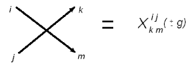
One can treat Xโ€‹(ยฑg2)๐‘‹plus-or-minussuperscript๐‘”2X(\pm g^{2}) as an operator acting in the space R1โŠ—R2tensor-productsubscript๐‘…1subscript๐‘…2R_{1}\otimes R_{2}. It is convenient to consider the operator X๐‘‹X as a tensor with four indexes Xkโ€‹miโ€‹jsubscriptsuperscript๐‘‹๐‘–๐‘—๐‘˜๐‘šX^{i\,j}_{k\,m}, so that each index is associated with a leg of intersection vertex fig.4.
Refer to caption
Figure 4: Representation of intersection operator X๐‘‹X
Refer to caption
Figure 5: The contribution coming from two adjacent points of a link

The main feature of this operator is that the two adjacent point contribution can be simply expressed as corresponding product of two such operators fig.5.

4.2 The vev of the trefoil knot in Gโ€‹Lโ€‹(2)๐บ๐ฟ2GL(2) case

As a more explicit example let us consider how the intersection point operator (30) can be used for calculation of the kernels of polynomial invariants. Let us summate the series (30) for operators Fasuperscript๐น๐‘ŽF^{a} in fundamental representation of gโ€‹lโ€‹(2)๐‘”๐‘™2gl(2). In this case we have:

Xโ€‹(g2)=Xโ€‹(g2)=โˆ‘k=0โˆžg2โ€‹kk!โ€‹{Fa1โ€‹Fa2โ€‹โ€ฆโ€‹Fak}โŠ—2=Aโ€‹(g2)โ€‹I^โ€‹d+Bโ€‹(g2)โ€‹P^๐‘‹superscript๐‘”2๐‘‹superscript๐‘”2superscriptsubscript๐‘˜0superscript๐‘”2๐‘˜๐‘˜superscriptsuperscript๐นsubscript๐‘Ž1superscript๐นsubscript๐‘Ž2โ€ฆsuperscript๐นsubscript๐‘Ž๐‘˜tensor-productabsent2๐ดsuperscript๐‘”2^๐ผ๐‘‘๐ตsuperscript๐‘”2^๐‘ƒX(g^{2})=X(g^{2})=\sum_{k=0}^{\infty}\dfrac{g^{2k}}{k!}\{F^{a_{1}}\,F^{a_{2}}...\,F^{a_{k}}\}^{\otimes 2}=A(g^{2})\,{\hat{I}d}+B(g^{2})\,{\hat{P}} (31)

where I^โ€‹d^๐ผ๐‘‘{\hat{I}d}, P^^๐‘ƒ{\hat{P}} are the identity and interchange operators in โ„‚2โŠ—โ„‚2tensor-productsuperscriptโ„‚2superscriptโ„‚2\mathbb{C}^{2}\otimes\mathbb{C}^{2} and:

Aโ€‹(g2)=1/6โ€‹eg2+1/6โ€‹eg2โ€‹g2+5/6โˆ’1/3โ€‹g2,๐ดsuperscript๐‘”216superscript๐‘’superscript๐‘”216superscript๐‘’superscript๐‘”2superscript๐‘”25613superscript๐‘”2A(g^{2})=1/6\,{e^{g^{2}}}+1/6\,{e^{g^{2}}}g^{2}+5/6-1/3\,g^{2},
Bโ€‹(g2)=2/3โ€‹eg2โˆ’2/3+1/6โ€‹g2+1/6โ€‹eg2โ€‹g2๐ตsuperscript๐‘”223superscript๐‘’superscript๐‘”22316superscript๐‘”216superscript๐‘’superscript๐‘”2superscript๐‘”2B(g^{2})=2/3\,{e^{g^{2}}}-2/3+1/6\,g^{2}+1/6\,{e^{g^{2}}}g^{2}
I^โ€‹d=[1000010000100001],P^=[1000001001000001]formulae-sequence^๐ผ๐‘‘delimited-[]1000missing-subexpression0100missing-subexpression0010missing-subexpression0001^๐‘ƒdelimited-[]1000missing-subexpression0010missing-subexpression0100missing-subexpression0001{\hat{I}d}=\left[\begin{array}[]{cccc}1&0&0&0\\ \vskip 6.0pt plus 2.0pt minus 2.0pt\cr 0&1&0&0\\ \vskip 6.0pt plus 2.0pt minus 2.0pt\cr 0&0&1&0\\ \vskip 6.0pt plus 2.0pt minus 2.0pt\cr 0&0&0&1\end{array}\right],\ \ \ \ {\hat{P}}=\left[\begin{array}[]{cccc}1&0&0&0\\ \vskip 6.0pt plus 2.0pt minus 2.0pt\cr 0&0&1&0\\ \vskip 6.0pt plus 2.0pt minus 2.0pt\cr 0&1&0&0\\ \vskip 6.0pt plus 2.0pt minus 2.0pt\cr 0&0&0&1\end{array}\right]
Refer to caption
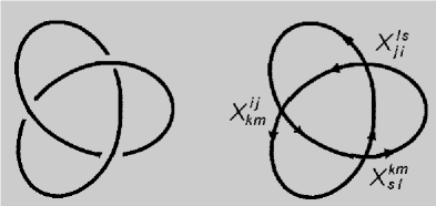
Figure 6: Two dimensional projection of the trefoil knot and contraction of intersection operators.

To find the kernel of polynomial invariant, for example of the trefoil knot, we need to chose some projection of the knot to two-dimensional plane. For instance as in the fig.6. Then, we attach to every intersection point of obtained two-dimensional curve the tensor Xโ€‹(ฯตโ€‹g2)๐‘‹italic-ฯตsuperscript๐‘”2X(\epsilon g^{2}), where ฯตitalic-ฯต\epsilon is the sign of the intersection point defined byย (12). Finally, to find the kernel of polynomial invariant in this case, we contract the indexes of the tensors in accordance with two dimensional diagram fig.6:

<W^โ€‹(31)>=โˆ‘iโ€‹jโ€‹kโ€‹mโ€‹sโ€‹lXkโ€‹miโ€‹jโ€‹Xsโ€‹lkโ€‹mโ€‹Xjโ€‹klโ€‹s=expectation^๐‘Šsubscript31subscript๐‘–๐‘—๐‘˜๐‘š๐‘ ๐‘™subscriptsuperscript๐‘‹๐‘–๐‘—๐‘˜๐‘šsubscriptsuperscript๐‘‹๐‘˜๐‘š๐‘ ๐‘™subscriptsuperscript๐‘‹๐‘™๐‘ ๐‘—๐‘˜absent<\hat{W}(3_{1})>=\sum\limits_{i\,j\,\,k\,m\,s\,l}X^{i\,j}_{k\,m}\,X^{k\,m}_{s\,l}\,X^{l\,s}_{j\,k}=
2โ€‹(5/6โ€‹eg2+1/3โ€‹eg2โ€‹g2+1/6โˆ’1/6โ€‹g2)3+limit-from2superscript56superscript๐‘’superscript๐‘”213superscript๐‘’superscript๐‘”2superscript๐‘”21616superscript๐‘”232\,(5/6\,{e^{{g}^{2}}}+1/3\,{e^{{g}^{2}}}{g}^{2}+1/6-1/6\,{g}^{2})^{3}+
+6โ€‹(1/6โ€‹eg2+1/6โ€‹eg2โ€‹g2+5/6โˆ’1/3โ€‹g2)2โ€‹(2/3โ€‹eg2โˆ’2/3+1/6โ€‹g2+1/6โ€‹eg2โ€‹g2)+limit-from6superscript16superscript๐‘’superscript๐‘”216superscript๐‘’superscript๐‘”2superscript๐‘”25613superscript๐‘”2223superscript๐‘’superscript๐‘”22316superscript๐‘”216superscript๐‘’superscript๐‘”2superscript๐‘”2+6\,(1/6\,{e^{{g}^{2}}}+1/6\,{e^{{g}^{2}}}{g}^{2}+5/6-1/3\,{g}^{2})^{2}(2/3\,{e^{{g}^{2}}}-2/3+1/6\,{g}^{2}+1/6\,{e^{{g}^{2}}}{g}^{2})+ (32)
+2โ€‹(2/3โ€‹eg2โˆ’2/3+1/6โ€‹g2+1/6โ€‹eg2โ€‹g2)32superscript23superscript๐‘’superscript๐‘”22316superscript๐‘”216superscript๐‘’superscript๐‘”2superscript๐‘”23+2\,(2/3\,{e^{{g}^{2}}}-2/3+1/6\,{g}^{2}+1/6\,{e^{{g}^{2}}}{g}^{2})^{3}

The expansion of <W^โ€‹(31)>expectation^๐‘Šsubscript31<\hat{W}(3_{1})> in g2superscript๐‘”2g^{2} coincide precisely with the result obtained in section 3.13.13.1 for the trefoil knot 31subscript313_{1} in the N=2๐‘2N=2 case by means of Labastida-Pรฉrez formula:

<W^โ€‹(31)>=2+12โ€‹g2+272โ€‹g4+19โ€‹g6+734โ€‹g8+27920โ€‹g10+Oโ€‹(g12)expectation^๐‘Šsubscript31212superscript๐‘”2272superscript๐‘”419superscript๐‘”6734superscript๐‘”827920superscript๐‘”10๐‘‚superscript๐‘”12<\hat{W}(3_{1})>=2+12\,g^{2}+{\frac{27}{2}}{g}^{4}+19\,{g}^{6}+{\frac{73}{4}}{g}^{8}+{\frac{279}{20}}{g}^{10}+O({g}^{12})

Therefore, we observed an interesting property of CS theory in the temporal gauge with the propagator (6): the vevs of Wilson loops are factorized into the product of the intersection point operators corresponding to the crossings of two-dimensional projection of the knot. We note that in this case the vevs of Wilson loops are not knot invariants and depends on the projection chosen, moreover, the kernels of the polynomial invariants are not polynomials in eg2superscript๐‘’superscript๐‘”2e^{g^{2}} anymore (as it could be seen from (32)).
Of course, without the prescription depending term in the propagator (5) the theory is incomplete, and appropriate choice for this term is needed. Nevertheless, the first term of the propagator (5) that we used in this work, contains only information about crossings, and the second, prescription depending term, does not depend on the crossing sings, as it does not depend on x0subscript๐‘ฅ0x_{0}. This leads us to the conjecture, that in the presence of the prescription depending term, the property of vevs to be factorized into the product of some tensors corresponding to crossings, should be conserved.

5 Conclusion

There are a lot of the combinatorial constructions for the knot polynomial invariants in terms of regular two-dimensional projections. For example the Jones polynomial arising from the braid group representations [9] or the Kauffman construction of Jones polynomials in terms of R๐‘…R-matrices and the โ€creation-annihilationโ€ operators [5]. All this constructions provide some tensors corresponding to intersection points, and some additional tensors corresponding to free lines, like the Kauffman โ€creationโ€ and โ€annihilationโ€ operators which correspond to critical points of the knots in the Morse representation. The natural way for deriving these representations form CS theory is to use the temporal gauge fixing as the perturbation theory in this gauge depends only on two-dimensional representation of the knot. The CS theory in the temporal gauge with propagator (6) contains only information about crossings, and operators corresponding to the Kauffman creation annihilation operators can not be derived by means of this propagator. In this way, we should conclude, that the prescription depending term in (5) plays a crucial role in the construction of correct perturbation theory for CS in the temporal gauge.
To find exact expression for this term we need some additional physical restrictions on the form of the propagator. As an example of such a restriction we can demand that the propagator gives the perturbative series expansion for Wilson lines is in agreement with some general properties of CS theory, for example the factorization theorem [12]-[14]. The examples of restrictions on prescription depending term arising from factorization theorem can be found in [13]. Another example of restriction gives consideration of the unknot vevs for a projection without intersection points. In this case the first term of the propagator (5) does not play any role and the perturbation series expansion contains only multidimensional integrals on products of prescription depending terms. We should demand that this series expansion coincides with the known series for vevs of unknot. All this will be considered elsewhere.


Acknowledgments

The author is grateful to A.Morozov for fruitful discussions and interest to this work. The work was partly supported by RFBR grant 09-02-00393, RFBR grant 06-01-92054-Kโ€‹Ea๐พsubscript๐ธ๐‘ŽKE_{a}, RFBR-CNRS grant 09-01-93106, and grant for support of scientific schools NSh-3036.2008.2. The work was also supported in part by the โ€Dynastyโ€ Foundation.

References

  • [1] E.Witten, Commun.Math.Phys. 121, 351-399 (1989)
  • [2] V.F.R. Jones, Bull. AMS 12 (1985) 103; Ann. of Math. 126 (1987) 335.
  • [3] P.Freyd, D.Yetter, J.Hoste, W.B.R.Lickorish, K.Millet, and A.Ocneanu, Bull. AMS 12 (1985) 239.
  • [4] Y.Akutsu and M. Wadati, J.Phus.Soc.Jap. 56 (1987) 839 and 3039
  • [5] L.H.Kauffman, Note di Matematica vol. 9 17-32 (1989)
  • [6] L.H.Kauffman, Trans, Am. Math. Soc. 318 (1990) 417
  • [7] D.Bar-Natan, Ph.D. Thesis, Princeton Univericity (1991).
  • [8] E.Guadagnini, M.Martellini and Mitchev, Phys.Lett.B227 (1989) 111; B228 (1989) 489; Nucl.Phys. B330 (1990) 575.
  • [9] E.Guadagnini, CERN-TH 5827-90 (1990)
  • [10] A. Morozov, A. Rosly, early 90โ€™s, unpublished
  • [11] M.Alvarez, and J.M.F.Labastida, Nucl. Phys. B395,(1993) 198; B433 (1995) 555.
  • [12] J.M.F.Labastida and E.Pรฉrez, Nucl.Phys. B527, (1998) 499;
  • [13] J.M.F.Labastida and E.Pรฉrez, CERN-TH/98-193, US-FT-11/98 (1998) 499;
  • [14] J.M.F.Labastida and E.Pรฉrez, Journ.Math.Phys. 39, (1998) 5183
  • [15] T.Dimofte, S. Gukov, J. Lenells, D.Zagier, arXiv: hep-th 0903.2472v1 (2009)
  • [16] A.S.Cattaneo, P.Cotta-Ramusino, J.Frohlich and M. Martellini, Jour.Math.Phys. 36 (1995) 6137.
  • [17] V.A. Vassiliev, Amer. Math. Soc., Providence, RI, (1990), 23
  • [18] V.A.Vassiliev, Translation of Mathematical Monographs, vol.98, AMS, (1992)
  • [19] R.Bott and C.Taubes, Jour.Math.Phys. 35 (1994) 5247.
  • [20] M.Kontsevich, Advances in Soviet Math. 16, part 2 (1993) 137
  • [21] I.A. Dynnikov, Funkts. Anal. Prilozh. vol. 33, 25-37, (1999)