Direct Determination of the Solar Neutrino Fluxes from Solar Neutrino Data

Abstract:

We determine the solar neutrino fluxes from a global analysis of the solar and terrestrial neutrino data in the framework of three-neutrino mixing. Using a Bayesian approach we reconstruct the posterior probability distribution function for the eight normalization parameters of the solar neutrino fluxes plus the relevant masses and mixing, with and without imposing the luminosity constraint. This is done by means of a Markov Chain Monte Carlo employing the Metropolis-Hastings algorithm. We also describe how these results can be applied to test the predictions of the Standard Solar Models. Our results show that, at present, both models with low and high metallicity can describe the data with good statistical agreement.

1 Introduction

The idea that the Sun generates power through nuclear fusion in its core was first suggested in 1919 by Sir Arthur Eddington who pointed out that the nuclear energy stored in the Sun could explain the apparent age of the Solar System. In 1939, Hans Bethe described in an epochal paper [1] two nuclear fusion mechanisms by which main sequence stars like the Sun could produce the energy necessary to power their observed luminosities. The two mechanisms have become known as the pp-chain and the CNO-cycle [2]. For both chains the basic energy source is the burning of four protons to form an alpha particle, two positrons, and two neutrinos. In the pp-chain, fusion reactions among elements lighter than $A=8$ produce a characteristic set of neutrino fluxes, whose spectral energy shapes are known but whose fluxes must be calculated with a detailed solar model. In the CNO-cycle the abundance of $\mbox{}^{12}\text{C}$ plus $\mbox{}^{13}\text{N}$ acts as a catalyst, while the $\mbox{}^{13}\text{N}$ and $\mbox{}^{15}\text{O}$ beta decays provide the primary source of neutrinos.

In order to precisely determine the rates of the different reactions in the two chains, which are responsible for the final neutrino fluxes and their energy spectrum, a detailed knowledge of the Sun and its evolution is needed. Standard Solar Models (SSM’s) [3, 4, 5, 6, 7, 8, 9] describe the properties of the Sun and its evolution after entering the main sequence. The models are based on a set of observational parameters (the present surface abundances of heavy elements and surface luminosity of the Sun, as well as its age, radius and mass) and on several basic assumptions: spherical symmetry, hydrostatic and thermal equilibrium, and equation of state. Over the past five decades the solar models were steadily refined as the result of increased observational and experimental information about the input parameters (such as nuclear reaction rates and the surface abundances of different elements), more accurate calculations of constituent quantities (such as radiative opacity and equation of state), the inclusion of new physical effects (such as element diffusion) and the development of faster computers and more precise stellar evolution codes.

Despite the progress of the theory, only neutrinos, with their extremely small interaction cross sections, can enable us to see into the interior of a star and thus verify directly our understanding of the Sun [10]. Indeed from the earliest days of solar neutrino research this test has been a primary goal of solar neutrino experiments, but for many years the task was made difficult by the increasing discrepancy between the predictions of the SSM’s and the solar neutrino observations. This so-called “solar neutrino problem” [11, 12] was finally solved by the modification of the Standard Model of Particle Physics with the inclusion of neutrino masses and mixing. In this new framework leptonic flavors are no longer symmetries of Nature, and neutrinos can change their flavor from the production point in the Sun to their detection on the Earth. This flavor transition probability is energy dependent [13, 14, 15, 16], which explains the apparent disagreement among experiments with different energy windows. This mechanism is known as the LMA-MSW solution to the solar neutrino problem, and affects both the overall number of events in solar neutrino experiments and the relative contribution expected from the different components of the solar neutrino spectrum. Due to these complications, at first it was necessary to assume the SSM predictions for all the solar neutrino fluxes and their uncertainties in order to extract reasonably constrained values for neutrino masses and mixing. The upcoming of the real-time experiments Super-Kamiokande and SNO and the independent determination of the flavor oscillation probability using reactor antineutrinos at KamLAND opened up the possibility of extracting the solar neutrino fluxes and their uncertainties directly from the data [17, 18, 19, 20, 21, 22, 9]. Nevertheless, in these works some set of simplifying assumptions had to be imposed in order to reduce the number of free parameters to be determined.

In parallel to the increased precision of the SSM-independent determination of the neutrino flavor parameters, a new puzzle has emerged in the consistency of SSM’s [23]. Till recently SSM’s have had notable successes in predicting other observations. In particular, quantities measured by helioseismology such as the radial distributions of sound speed and density [5, 6, 7, 8] showed good agreement with the predictions of the SSM calculations and provided accurate information on the solar interior. A key element to this agreement is the input value of the abundances of heavy elements on the surface of the Sun [24]. However, recent determinations of these abundances point towards substantially lower values than previously expected [25, 26]. A SSM which incorporates such lower metallicities fails at explaining the helioseismological observations [23], and changes in the Sun modeling (in particular of the less known convective zone) are not able to account for this discrepancy [27, 28].

So far there has not been a successful solution of this puzzle. Thus the situation is that, at present, there is no fully consistent SSM. This led to the construction of two different sets of SSM’s, one (labeled “GS”) based on the older solar abundances [24] implying high metallicity, and one (labeled “AGS”) assuming lower metallicity as inferred from more recent determinations of the solar abundances [25, 26]. In Ref. [9] the solar fluxes corresponding to such two models were detailed, based on updated versions of the solar model calculations presented in Ref. [8]. These fluxes were denoted as “BPS08(GS)” and “BPS08(AGS)”, respectively. In a very recent work [29] an update of the BPS08(AGS) solar model has been constructed using the latest determination of the compositions [26] as well as some improvement in the equation of state. For what concerns the overall normalization of solar neutrino fluxes, the predictions of this new model are very close to those of BPS08(AGS).

In this work we perform a solar model independent analysis of the solar and terrestrial neutrino data in the framework of three-neutrino masses and mixing. The aim of this analysis is to simultaneously determine the flavor parameters and all the solar neutrino fluxes with a minimum set of theoretical priors. In Sec. 2 we present the method employed, the data included in the analysis and the physical assumptions used in this study. The results of the analysis are given in Sec. 3, where we show the reconstructed posterior probability distribution function for the eight normalization parameters of the solar neutrino fluxes. We discuss in detail the effect of the luminosity constraint [30] as well as the role of the Borexino experiment and its potential for improvement. In addition, we use the results of this analysis to statistically test to what degree the present solar neutrino data can discriminate between the two SSM’s. Finally in Sec. 4 we summarize our conclusions.

2 Data analysis

In the analysis of solar neutrino experiments we include the total rates from the radiochemical experiments Chlorine [31], Gallex/GNO [32] and SAGE [32, 33]. For real-time experiments in the energy range of $\mbox{}^{8}\text{B}$ neutrinos we include the 44 data points of the electron scattering (ES) Super-Kamiokande phase I (SK-I) energy-zenith spectrum [34], the 34 data points of the day-night spectrum from SNO-I [35], the separate day and night rates for neutral current (NC) and ES events and the day-night energy-spectrum for charge current (CC) events from SNO-II (a total of 38 data points) [36], the three rates for CC, ES and NC from SNO-III [37], and the 6 points of the high-energy spectrum from the 246 live days of Borexino [38] (which we denote as Borexino-HE). Finally, we include the main set of the 192 days of Borexino data (denoted as Borexino-LE) [40] in two different forms: in one analysis we use the total event rates from $\mbox{}^{7}\text{Be}$ neutrinos as extracted by the Borexino collaboration, while in the other we perform our own fit to the Borexino energy spectrum in the region above $365$ keV (corresponding to a total of 160 data points). Full details of our Borexino data analysis are presented in Appendix A. In the framework of three neutrino masses and mixing the expected values for these solar neutrino observables depend on the parameters $\Delta m^{2}_{21}$, $\theta_{12}$, and $\theta_{13}$ as well as on the normalizations of the eight solar fluxes.

Besides solar experiments, we also include the latest results from the long baseline reactor experiment KamLAND [41, 42], which in the framework of three neutrino mixing also yield information on the parameters $\Delta m^{2}_{21}$, $\theta_{12}$, and $\theta_{13}$. In addition, we include the information on $\theta_{13}$ obtained after marginalizing over $\Delta m^{2}_{31}$, $\theta_{23}$ and $\delta_{\textsc{cp}}$ the results from the complete SK-I and SK-II atmospheric neutrino data sets (see the Appendix of Ref. [42] for full details on our analysis), the CHOOZ reactor experiment [43], K2K [44], the latest MINOS $\nu_{\mu}$ disappearance data corresponding to an exposure of $3.4\times 10^{20}$ p.o.t. [45], and the first MINOS $\nu_{\mu}\to\nu_{e}$ appearance data presented in Ref. [46]. Details of the oscillation analysis of these observables will be presented elsewhere [47].

Flux	$\Phi_{i}^{\text{ref}}$ [$\text{cm}^{-2}\,\text{s}^{-1}$]	$\alpha_{i}$ [MeV]	$\beta_{i}$
pp	$5.97\times 10^{10}$	$13.0987$	$9.171\times 10^{-1}$
$\mbox{}^{7}\text{Be}$	$5.07\times 10^{9\hphantom{0}}$	$12.6008$	$7.492\times 10^{-2}$
pep	$1.41\times 10^{8\hphantom{0}}$	$11.9193$	$1.971\times 10^{-3}$
$\mbox{}^{13}\text{N}$	$2.88\times 10^{8\hphantom{0}}$	$\hphantom{0}3.4577$	$1.168\times 10^{-3}$
$\mbox{}^{15}\text{O}$	$2.15\times 10^{8\hphantom{0}}$	$21.5706$	$5.439\times 10^{-3}$
$\mbox{}^{17}\text{F}$	$5.82\times 10^{6\hphantom{0}}$	$\hphantom{0}2.363\hphantom{0}$	$1.613\times 10^{-5}$
$\mbox{}^{8}\text{B}$	$5.94\times 10^{6\hphantom{0}}$	$\hphantom{0}6.6305$	$4.619\times 10^{-5}$
hep	$7.90\times 10^{3\hphantom{0}}$	$\hphantom{0}3.7370$	$3.462\times 10^{-8}$

Table 1: The reference neutrino flux $\Phi_{i}^{\text{ref}}$ used for normalization, the energy $\alpha_{i}$ provided to the star by nuclear fusion reactions associated with the $i^{\text{th}}$ neutrino flux (taken from Ref. [30]), and the fractional contribution $\beta_{i}$ of the $i^{\text{th}}$ nuclear reaction to the total solar luminosity.

In what follows, for convenience, we will use as normalization parameters for the solar fluxes the reduced quantities:

$$f_{i}=\frac{\Phi_{i}}{\Phi_{i}^{\text{ref}}}$$ (1)

with $i={\text{pp}}$, $\mbox{}^{7}\text{Be}$, pep, $\mbox{}^{13}\text{N}$, $\mbox{}^{15}\text{O}$, $\mbox{}^{17}\text{F}$, $\mbox{}^{8}\text{B}$, and hep. The numerical values of $\Phi_{i}^{\text{ref}}$ are conventionally set to the predictions of the BPS08(GS) solar model and are listed in Table 1. With this, the theoretical predictions for the relevant observables (after marginalizing over $\Delta m^{2}_{23}$, $\theta_{23}$ and $\delta_{\textsc{cp}}$) depend on eleven parameters: the three relevant oscillation parameters $\Delta m^{2}_{21}$, $\theta_{12}$, $\theta_{13}$ and the eight reduced solar fluxes $f_{i}$. With the data from the different data samples (D) and the theoretical predictions for them in terms of these parameters $\vec{\omega}=(\Delta m^{2}_{21},\theta_{12},\theta_{13},f_{{\text{pp}}},\dots,f_{{\text{hep}}})$ we build the corresponding likelihood function

$$\mathcal{L}(\mathrm{D}|\vec{\omega})=\frac{1}{N}\exp\left[-\frac{1}{2}\chi^{2}(\mathrm{D}|\vec{\omega})\right]$$ (2)

where $N$ is a normalization factor. In Bayesian statistics our knowledge of $\vec{\omega}$ is summarized by the posterior probability distribution function (p.d.f.)

$$p(\vec{\omega}|\mathrm{D},\mathcal{P})=\dfrac{\mathcal{L}(\mathrm{D}|\vec{\omega})\,\pi(\vec{\omega}|\mathcal{P})}{\int\mathcal{L}(\mathrm{D}|\vec{\omega}^{\prime})\,\pi(\vec{\omega}^{\prime}|\mathcal{P})\,d\vec{\omega}^{\prime}}$$ (3)

where $\pi(\vec{\omega}|\mathcal{P})$ is the prior probability density for the parameters. In our model independent analysis we assume a uniform prior probability over which we impose the following set of constraints to ensure consistency in the pp-chain and CNO-cycle, as well as some relations from nuclear physics:

• The fluxes must be positive:

  $$\Phi_{i}\geq 0\quad\Rightarrow\quad f_{i}\geq 0\,.$$ (4)

• The number of nuclear reactions terminating the pp-chain should not exceed the number of nuclear reactions which initiate it [48, 30]:

  $$\Phi_{{\mbox{}^{7}\text{Be}}}+\Phi_{{\mbox{}^{8}\text{B}}}\leq\Phi_{{\text{pp}}}+\Phi_{{\text{pep}}}\\ \Rightarrow\quad 8.49\times 10^{-2}f_{{\mbox{}^{7}\text{Be}}}+9.95\times 10^{-5}f_{{\mbox{}^{8}\text{B}}}\leq f_{{\text{pp}}}+2.36\times 10^{-3}f_{{\text{pep}}}\,.$$ (5)

• The ${\mbox{}^{14}\text{N}}(p,\gamma){\mbox{}^{15}\text{O}}$ reaction must be the slowest process in the main branch of the CNO-cycle [48]:

  $$\Phi_{{\mbox{}^{15}\text{O}}}\leq\Phi_{{\mbox{}^{13}\text{N}}}\quad\Rightarrow\quad f_{{\mbox{}^{15}\text{O}}}\leq 1.34f_{{\mbox{}^{13}\text{N}}}$$ (6)

  and the CNO-II branch must be subdominant:

  $$\Phi_{{\mbox{}^{17}\text{F}}}\leq\Phi_{{\mbox{}^{15}\text{O}}}\quad\Rightarrow\quad f_{{\mbox{}^{17}\text{F}}}\leq 37f_{{\mbox{}^{15}\text{O}}}\,.$$ (7)

• The ratio of the pep neutrino flux to the pp neutrino flux is fixed to high accuracy because they have the same nuclear matrix element. We have constrained this ratio to match the average of the BPS08(GS) and BPS08(AGS) values, with $1\sigma$ Gaussian uncertainty given by the difference between the values in the two models

  $$\frac{f_{{\text{pep}}}}{f_{{\text{pp}}}}=1.008\pm 0.010\,.$$ (8)

Following standard techniques we reconstruct the posterior p.d.f. in Eq. (3) using a Monte-Carlo algorithm; full details of our approach are given in Appendix B.

The number of independent fluxes is reduced when imposing the so-called “luminosity constraint”, i.e., the requirement that the sum of the thermal energy generation rates associated with each of the solar neutrino fluxes coincides with the solar luminosity [49]:

$$\frac{L_{\odot}}{4\pi\,(\text{A.U.})^{2}}=\sum_{i=1}^{8}\alpha_{i}\Phi_{i}\,.$$ (9)

Here the constant $\alpha_{i}$ is the energy provided to the star by the nuclear fusion reactions associated with the $i^{\text{th}}$ neutrino flux; its numerical value is independent of details of the solar model to an accuracy of one part in $10^{4}$ or better [30]. A detailed derivation of this equation and the numerical values of the coefficients $\alpha_{i}$, which we reproduce for convenience in Table 1, is presented in Ref. [30]. In terms of the reduced fluxes Eq. (9) can be written as:

$$1=\sum_{i=1}^{8}\beta_{i}f_{i}\quad\text{with}\quad\beta_{i}\equiv\frac{\alpha_{i}\Phi_{i}^{\text{ref}}}{L_{\odot}\big{/}[4\pi\,(\text{A.U.})^{2}]}$$ (10)

where $\beta_{i}$ is the fractional contribution to the total solar luminosity of the nuclear reactions responsible for the production of the $\Phi_{i}^{\text{ref}}$ neutrino flux, and $L_{\odot}\big{/}[4\pi\,(\text{A.U.})^{2}]=8.5272\times 10^{11}\,\text{MeV}\,\text{cm}^{-2}\,\text{s}^{-1}$ [30]. The analysis performed incorporating the priors in Eqs. (4–9) will be named “analysis with luminosity constraint”, $\mathcal{P}=L_{\odot}$, and for this case the prior probability distribution is:

$$\pi(\vec{\omega}^{\prime}|L_{\odot})=\begin{cases}\dfrac{1}{N}\exp\left[-\dfrac{\left(f_{{\text{pep}}}\big{/}f_{{\text{pp}}}-1.008\right)^{2}}{2\sigma^{2}}\right]&\text{if Eqs.~{}(\ref{eq:fpos}--\ref{eq:CNOineq2}) and~{}\eqref{eq:lumsum} are verified,}\\ 0&\text{otherwise,}\end{cases}$$ (11)

where $N$ is a normalization factor and $\sigma=0.010$. When only Eqs. (4–8) are imposed we will speak of “analysis without luminosity constraint”, $\mathcal{P}={\;/\!\!\!\!L}_{\odot}$, so:

$$\pi(\vec{\omega}^{\prime}|{{\;/\!\!\!\!L}_{\odot}})=\begin{cases}\dfrac{1}{N}\exp\left[-\dfrac{\left(f_{{\text{pep}}}\big{/}f_{{\text{pp}}}-1.008\right)^{2}}{2\sigma^{2}}\right]&\text{if Eqs.~{}(\ref{eq:fpos}--\ref{eq:CNOineq2}) are verified,}\\ 0&\text{otherwise.}\end{cases}$$ (12)

Let us notice that the conditions in Eqs. (4–7) and Eq. (9) are constraints on some linear combinations of the solar fluxes and they are model independent, i.e., they do not impose any prior bias favouring either of the SSM’s. Furthermore we have chosen to center the condition (8) at the average of the BPS08(GS) and BPS08(AGS) values, with $1\sigma$ Gaussian uncertainty given by the difference between the values in the two models, to avoid the introduction of a bias towards one of the models. In the next sections we will comment on how our results are affected when this prior is centered about the BPS08(GS) or the BPS08(AGS) prediction.

3 Results

Figure 1: Constraints from our global analysis on the solar neutrino fluxes. The curves in the rightmost panels show the marginalized one-dimensional probability distributions, before and after the inclusion of the Borexino spectral data. The rest of the panels show the 90% and 99% CL two-dimensional credibility regions (see text for details).

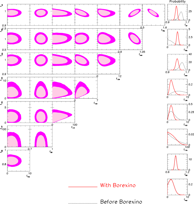
Our results for the analysis with luminosity constraint are displayed in Fig. 1, where we show the marginalized one-dimensional probability distributions $p(f_{i}|\mathrm{D},L_{\odot})$ for the eight solar neutrino fluxes as well as the 90% and 99% CL two-dimensional allowed regions. The corresponding ranges at $1\sigma$ (and at the 99% CL in square brackets) on the oscillation parameters are:

$$\Delta m^{2}_{21} =7.6\pm 0.2\,[\pm 0.5]\times 10^{-5}~{}\text{eV}^{2}\,,$$ (13)

$$\sin^{2}\theta_{12} =0.33\pm 0.02\,[\pm 0.05]\,,$$

$$\sin^{2}\theta_{13} =0.02\pm 0.012\,[^{+0.03}_{-0.02}]\,,$$

while for the solar neutrino fluxes are:

$$f_{{\text{pp}}} =0.990^{+0.010}_{-0.009}\,[^{+0.023}_{-0.030}]\,,\qquad \Phi_{{\text{pp}}} =5.910^{+0.057}_{-0.063}[^{+0.14}_{-0.16}]\times 10^{10}~{}\text{cm}^{-2}~{}\text{s}^{-1}\,,$$ (14)

$$f_{{\mbox{}^{7}\text{Be}}} =1.00^{+0.10}_{-0.09}\,[^{+0.25}_{-0.21}]\,,\qquad \Phi_{{\mbox{}^{7}\text{Be}}} =5.08^{+0.52}_{-0.43}\,[^{+1.3}_{-1.0}]\times 10^{9}~{}\text{cm}^{-2}~{}\text{s}^{-1}\,,$$

$$f_{{\text{pep}}} =0.998\pm 0.014\,[\pm 0.04]\,,\qquad \Phi_{{\text{pep}}} =1.407^{+0.019}_{-0.020}\,[^{+0.054}_{-0.057}]\times 10^{8}~{}\text{cm}^{-2}~{}\text{s}^{-1}\,,$$

$$f_{{\mbox{}^{13}\text{N}}} =2.7^{+1.7}_{-1.2}\,[^{+5.6}_{-2.4}]\,,\qquad \Phi_{{\mbox{}^{13}\text{N}}} =7.8^{+5.0}_{-3.4}\,[^{+16}_{-7.0}]\times 10^{8}~{}\text{cm}^{-2}~{}\text{s}^{-1}\,,$$

$$f_{{\mbox{}^{15}\text{O}}} =1.8\pm 0.9\,[^{+2.2}_{-1.8}]\,,\qquad \Phi_{{\mbox{}^{15}\text{O}}} =4.0^{+1.8}_{-1.9}\,[^{+4.8}_{-3.8}]\times 10^{8}~{}\text{cm}^{-2}~{}\text{s}^{-1}\,,$$

$$f_{{\mbox{}^{17}\text{F}}} \leq 32\,[72]\,,\qquad \Phi_{{\mbox{}^{17}\text{F}}} \leq 5.9\,[43]\times 10^{7}~{}\text{cm}^{-2}~{}\text{s}^{-1}\,,$$

$$f_{{\mbox{}^{8}\text{B}}} =0.85\pm 0.03\,[\pm 0.08]\,,\qquad \Phi_{{\mbox{}^{8}\text{B}}} =5.02^{+0.18}_{-0.17}\,[^{+0.45}_{-0.42}]\times 10^{6}~{}\text{cm}^{-2}~{}\text{s}^{-1}\,,$$

$$f_{{\text{hep}}} =1.7^{+1.3}_{-1.4}\,[^{+3.8}_{-1.7}]\,,\qquad \Phi_{{\text{hep}}} =1.3\pm 1.0\,[^{+3.0}_{-1.3}]\times 10^{4}~{}\text{cm}^{-2}~{}\text{s}^{-1}\,.$$

As mentioned above we have checked the stability of the results under changes in the assumption of the prior in Eq. (8). We find that if we center this prior at the BPS08(GS) prediction ($f_{{\text{pep}}}\big{/}f_{{\text{pp}}}=1$) the best fit value for pep neutrinos is changed to $f_{{\text{pep}}}=0.986$ ($\Phi_{{\text{pep}}}=1.390\times 10^{8}\,\text{cm}^{-2}\,\text{s}^{-1}$). Conversely if the Gaussian prior in Eq. (8) is centered at the BPS08(AGS) prediction ($f_{{\text{pep}}}\big{/}f_{{\text{pp}}}=1.016$) we get $f_{{\text{pep}}}=1.003$ ($\Phi_{{\text{pep}}}=1.414\times 10^{8}\,\text{cm}^{-2}\,\text{s}^{-1}$). All other fluxes are unaffected.

For the sake of illustration we have also performed a Gaussian fit to the two-dimensional p.d.f. for the eight fluxes. The best Gaussian approximation to the real p.d.f. is characterized by flux uncertainties obtained by symmetrizing the $1\sigma$ ranges quoted in Eq. (14), and by the following error correlation matrix:

$$\begin{array}[]{l|cccccccc}&f_{{\text{pp}}}&f_{{\mbox{}^{7}\text{Be}}}&f_{{\text{pep}}}&f_{{\mbox{}^{13}\text{N}}}&f_{{\mbox{}^{15}\text{O}}}&f_{{\mbox{}^{17}\text{F}}}&f_{{\mbox{}^{8}\text{B}}}&f_{{\text{hep}}}\\ \hline\cr f_{{\text{pp}}}&1&-0.81&\hphantom{+}0.74&-0.28&-0.64&-0.26&\hphantom{+}0.06&\hphantom{+}0.00\\ f_{{\mbox{}^{7}\text{Be}}}&&1&-0.58&-0.10&\hphantom{+}0.10&\hphantom{+}0.12&-0.05&\hphantom{+}0.00\\ f_{{\text{pep}}}&&&1&-0.22&-0.49&-0.20&\hphantom{+}0.04&\hphantom{+}0.01\\ f_{{\mbox{}^{13}\text{N}}}&&&&1&\hphantom{+}0.31&\hphantom{+}0.06&-0.02&\hphantom{+}0.00\\ f_{{\mbox{}^{15}\text{O}}}&&&&&1&\hphantom{+}0.30&-0.03&\hphantom{+}0.00\\ f_{{\mbox{}^{17}\text{F}}}&&&&&&1&-0.02&\hphantom{+}0.00\\ f_{{\mbox{}^{8}\text{B}}}&&&&&&&1&-0.04\\ f_{{\text{hep}}}&&&&&&&&1\end{array}$$ (15)

As seen in Fig. 1 and in Eq. (15) the most important correlation appears between the pp and pep fluxes, as expected from the relation (8). The correlation between the pp (and pep) and $\mbox{}^{7}\text{Be}$ flux is directly dictated by the luminosity constraint (see comparison with Fig. 3). All these results imply the following share of the energy production between the pp-chain and the CNO-cycle

$$\frac{L_{\text{pp-chain}}}{L_{\odot}}=0.986^{+0.005}_{-0.006}\,[^{+0.011}_{-0.014}]\quad\Longleftrightarrow\quad\frac{L_{\text{CNO}}}{L_{\odot}}=0.014^{+0.006}_{-0.005}\,[^{+0.014}_{-0.011}]\,,$$ (16)

in perfect agreement with the SSM’s which predict $L_{\text{CNO}}/L_{\odot}\leq 1$% at the $3\sigma$ level.

Figure 2: Contribution of each solar neutrino flux to the total event rates at different experiments. The oscillation parameters are set to their best fit value, Eq. (13). We show the contributions as predicted by BPS08(GS) and BPS08(AGS) solar models as well as our best fit values given in Eq. (14).

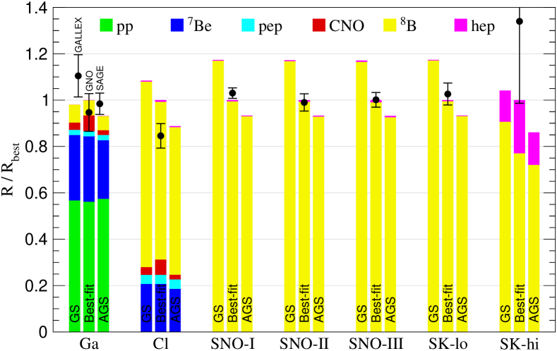
The sensitivity of the various experiments is illustrated in Fig. 2, where we plot the contribution of each flux to the total event rates at the radiochemical experiments as well as SNO and SK (for Borexino see Appendix A) together with the corresponding experimental values and uncertainties. To highlight the sensitivity to the hep flux we plot separately the rate for the last energy bin in SK (SK-hi, $E_{e}\geq 16$ MeV); similar results hold for the highest energy bins of SNO. The rates are computed for the best fit value of the oscillations parameters, Eq. (13). We show the contributions as predicted by BPS08(GS) and BPS08(AGS) solar models and by our best fit values for the fluxes given in Eq. (14).

Figure 3: Same as Fig. 1 but without the luminosity constraint, Eq. (9). The curves in the rightmost panels show the marginalized one-dimensional probability distributions, before and after the inclusion of the Borexino spectral data. The rest of the panels show the 90% and 99% CL two-dimensional credibility regions (see text for details).

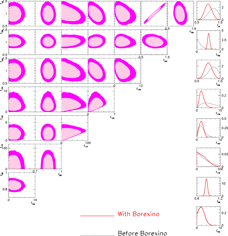
In order to check the consistency of our results we have performed the same analysis without imposing the luminosity constraint, Eq. (9). The corresponding results for $p(f_{i}|\mathrm{D},{\;/\!\!\!\!L}_{\odot})$ and the two-dimensional allowed regions are shown in Fig. 3. As expected, the pp flux is the most affected by the release of this constraint. This is so because the pp reaction gives the largest contribution to the solar energy production, as can be seen in Table 1. Imposing the luminosity constraint as an upper bound on the pp flux would imply that this flux cannot exceed its SSM prediction by more than 9%. Conversely, releasing this constraint allows for a much larger pp flux. The pep flux is also severely affected due to its strong correlation with the pp flux, Eq. (8). On a smaller scale the CNO fluxes are also affected, mainly as an indirect effect due to the modified contribution of the pp and pep fluxes to the Gallium and Chlorine experiments, which leads to a change in the allowed contribution of the CNO fluxes to these experiments. Thus in this case we get:

$$f_{{\text{pp}}}=f_{{\text{pep}}} =0.98^{+0.16}_{-0.15}\,[^{+0.47}_{-0.40}]\,,$$ (17)

$$f_{{\mbox{}^{7}\text{Be}}} =1.01^{+0.1}_{-0.09}\,[^{+0.27}_{-0.22}]\,,$$

$$f_{{\mbox{}^{13}\text{N}}} =2.7^{+1.8}_{-1.3}\,[^{+5.7}_{-2.5}]\,,$$

$$f_{{\mbox{}^{15}\text{O}}} =1.9\pm 1\,[^{+2.3}_{-1.9}]\,,$$

$$f_{{\mbox{}^{17}\text{F}}} \leq 34\,[79]\,.$$

The determination of the $\mbox{}^{8}\text{B}$ and hep fluxes (as well as the oscillation parameters) is basically unaffected by the luminosity constraint.

Interestingly, the idea that the Sun shines because of nuclear fusion reactions can be tested accurately by comparing the observed photon luminosity of the Sun with the luminosity inferred from measurements of solar neutrino fluxes. We find that the energy production in the pp-chain and the CNO-cycle without imposing the luminosity constraint are given by:

$$\frac{L_{\text{pp-chain}}}{L_{\odot}}=0.98^{+0.15}_{-0.14}\,[\pm 0.40]\qquad\text{and}\qquad\frac{L_{\text{CNO}}}{L_{\odot}}=0.015^{+0.005}_{-0.007}\,[^{+0.013}_{-0.014}]\,.$$ (18)

Comparing Eqs. (16) and (18) we see that the luminosity constraint has only a limited impact on the amount of energy produced in the CNO-cycle. However, as discussed above, the amount of energy in the pp-chain can now significantly exceed the total quantity allowed by the luminosity constraint. Altogether we find that the present value for the ratio of the neutrino-inferred solar luminosity, $L_{\odot}\text{(neutrino-inferred)}$, to the photon luminosity $L_{\odot}$ is:

$$\frac{L_{\odot}\text{(neutrino-inferred)}}{L_{\odot}}=1.00\pm 0.14\,[^{+0.37}_{-0.34}]\,.$$ (19)

Thus we find that, at present, the neutrino-inferred luminosity perfectly agrees with the measured one, and this agreement is known with a $1\sigma$ uncertainty of 14%.

3.1 The role and potential of Borexino

As seen in Figs. 1 and 3 the inclusion of Borexino has a very important impact on the determination of the $\mbox{}^{7}\text{Be}$, pep and CNO fluxes, and indirectly on the pp flux. As mentioned above and described in Appendix A, in our analysis we have fitted the 160 data points of the Borexino energy spectrum in the $365$–$2000$ keV energy range, leaving as free parameters the normalization of the the $\mbox{}^{11}\text{C}$, $\mbox{}^{14}\text{C}$, $\mbox{}^{210}\text{Bi}$ and $\mbox{}^{85}\text{Kr}$ backgrounds, the three relevant oscillation parameters, and the normalization of all the solar neutrino fluxes. In contrast, the Borexino collaboration fits the spectrum in the full energy range $160$–$2000$ keV, and allows for free normalizations of the $\mbox{}^{11}\text{C}$, $\mbox{}^{10}\text{C}$, $\mbox{}^{210}\text{Bi}$+CNO and $\mbox{}^{85}\text{Kr}$ backgrounds as well as $\mbox{}^{14}\text{C}$ (which introduces an overwhelming background but is only relevant for events below $250$ keV, hence it does not contribute to our analysis). Besides the normalization of these background components only the $\mbox{}^{7}\text{Be}$ flux normalization is fitted to the data, and no direct information on the normalization of the other solar fluxes is extracted. In particular, the CNO fluxes are added to the $\mbox{}^{210}\text{Bi}$ background and fitted as a unique “background”, while the other solar fluxes are fixed to the BPS08(GS) prediction and the oscillation parameters are fixed to the best fit point of the global pre-Borexino analysis. With this procedure they determine the interaction rate for the $0.862$ MeV $\mbox{}^{7}\text{Be}$ neutrinos to be $49\pm 3_{\text{stat}}\pm 4_{\text{sys}}$, which corresponds to $f_{{\mbox{}^{7}\text{Be}}}=1.02\pm 0.10$. Given the precision of the data and the energy spectrum of the irreducible backgrounds, their procedure is perfectly acceptable for the purpose of extracting the $\mbox{}^{7}\text{Be}$ normalization alone. However, in this work we are interested in testing the full set of SSM fluxes, not just $\mbox{}^{7}\text{Be}$. In this case the consistent procedure is to allow for independent normalizations of all the solar fluxes.

Figure 4: Marginalized one-dimensional probability distributions for the fluxes contributing to Borexino-LE. The full line shows the determination obtained by fitting the Borexino spectrum data as described in Appendix A. The dashed-dotted line shows what the results would be if instead one had used the Borexino result for the extracted interaction rate of the $0.862$ MeV $\mbox{}^{7}\text{Be}$ neutrinos. The dotted line represents the precision obtainable with the simulated “ideal” spectrum as described in Sec. 3.1.

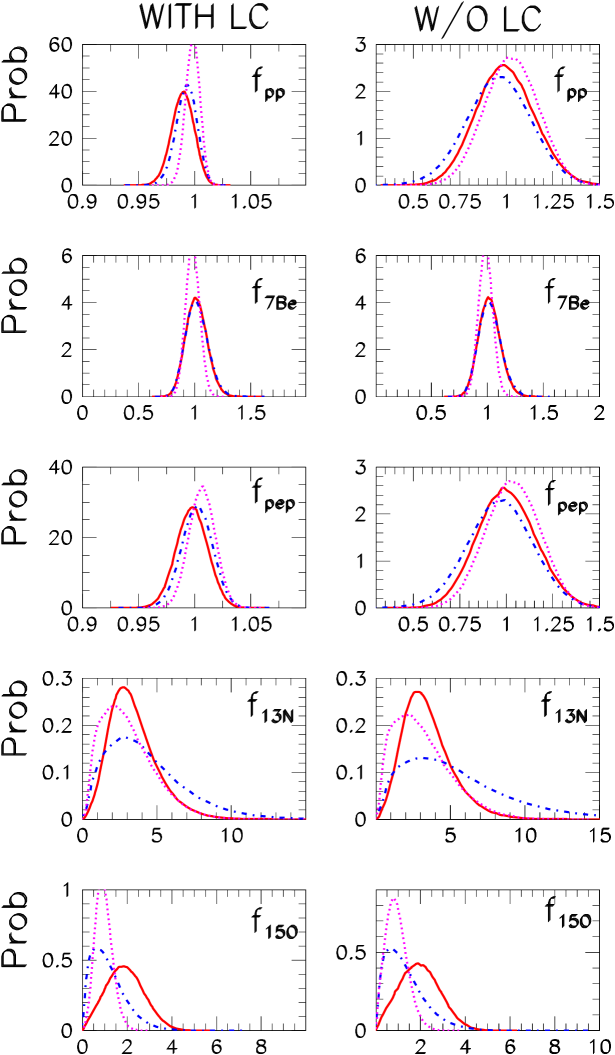
In order to illustrate the impact of these two different approaches on the determination of the SSM fluxes, we have repeated our analysis using as unique data input from Borexino-LE the total interaction rate for $\mbox{}^{7}\text{Be}$ neutrinos quoted by the collaboration. The results are shown in Fig. 4. As seen in this figure the constraints imposed on the $\mbox{}^{7}\text{Be}$ flux after the inclusion of Borexino are basically the same, irrespective of whether one includes the full Borexino energy spectrum in the range $365$–$2000$ keV or just the total $\mbox{}^{7}\text{Be}$ event rate extracted by the Borexino collaboration. However, the best fit and allowed ranges for the CNO fluxes are not the same. This proves that, despite the unknown level of $\mbox{}^{210}\text{Bi}$ contamination, the Borexino spectral data can still provide useful information on the CNO fluxes. When using only the total $\mbox{}^{7}\text{Be}$ event rate this information is lost and the constraints on CNO arise exclusively from the Gallium and Chlorine experiments.

As shown in Fig. 4, the inclusion of the complete Borexino-LE spectrum leads to an improvement (albeit not very significant) of the determination of the $\mbox{}^{13}\text{N}$ flux. Without Borexino this flux is mostly (and poorly) constrained by the Gallium experiment, and including the additional information from Borexino positively adds to its knowledge. We notice, however, that the best fit value of the $\mbox{}^{13}\text{N}$ flux in either analysis is always higher than the prediction of any of the SSM’s (although fully compatible at better than $1.5\sigma$). This behavior is driven by the Gallium rate which is slightly higher than expected in any of the SSM’s within the framework of three neutrino oscillations. A higher best fit value of $\mbox{}^{13}\text{N}$ can easily accommodate this observation without conflicting with any of the other experiments nor with the observed spectrum at Borexino. On the contrary, this is not the case for the $\mbox{}^{15}\text{O}$ flux. Adding the information from Borexino-LE spectrum leads to a (also small) worsening of the precision in the determination of this flux. We traced this apparently counter-intuitive result to the existing tension between the low Chlorine rate and the predicted rate within the framework of three neutrino oscillations. As a consequence of this tension, Chlorine pushes towards lower values of the $\mbox{}^{15}\text{O}$ flux, whereas the spectrum of Borexino-LE prefers a higher amount of $\mbox{}^{15}\text{O}$. When only the total event rate of $\mbox{}^{7}\text{Be}$ is used in the fit the extracted $\mbox{}^{15}\text{O}$ flux is mostly driven by the Chlorine result. When the Borexino-LE spectrum is also included the tension results into a higher best fit for the $\mbox{}^{15}\text{O}$ flux and a worsening of the precision.

Among all solar neutrino fluxes, the CNO ones are those for which the differences between the BPS08(GS) and BPS08(AGS) SSM predictions are largest. It is therefore interesting to explore whether this discrepancy can be resolved with future Borexino data, and to what degree the CNO and pep fluxes can be better determined. Besides the accumulation of more statistics, in the near future Borexino aims at reducing the systematic uncertainties with the deployment of calibration sources in the detector [40]. Ideally, if the $\mbox{}^{11}\text{C}$ background could be subtracted from the signal the pep and CNO fluxes would become directly accessible. In order to illustrate the potential of this perspective we have simulated an “ideal” spectrum of 85 bins in the energy range $365$–$1238$ keV according to the expectations from the central values of the BPS08(GS) fluxes and the best fit point of oscillations. In our simulation we have assumed that the $\mbox{}^{11}\text{C}$ has been fully removed, while the other backgrounds are added under the same assumptions as in the present Borexino analysis. We have also assumed double statistics and a reduction by a factor three of the systematic uncertainties. The results of this fit are presented in Fig. 4. As can be seen, with this ideal experiment the level of accuracy can be substantially improved for most fluxes, with the exception of $\mbox{}^{13}\text{N}$ flux whose determination becomes less precise. This is a consequence of the tension between the higher value of $\mbox{}^{13}\text{N}$ preferred by the Gallium experiments and the SSM value used for the simulated spectrum: if we had simulated data corresponding to a higher value of $\mbox{}^{13}\text{N}$ flux, the precision in the determination of this flux would also have improved. In any case, our results show that even with this optimistic improvement of Borexino the precision of the CNO fluxes remains far below the present uncertainties of the SSM’s.

3.2 Comparison with the Standard Solar Model(s)

Figure 5: Marginalized one-dimensional probability distributions for the best determined solar fluxes in our analysis as compared to the predictions for the two SSM’s in Ref. [9].

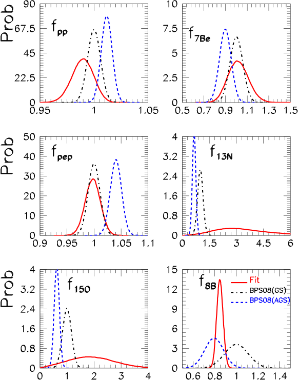
In Fig. 5 we show the marginalized one-dimensional probability distributions for the solar neutrino fluxes as determined by our analysis, together with the predictions for the two SSM’s given in Ref. [9]. In order to statistically compare our results with the SSM’s predictions we perform a significance test. We start by constructing a posterior probability distribution function for the solar fluxes as well as for the SSM central values. This is defined as the probability distribution from the data subject to the prior distribution of an arbitrary SSM:

$$p(\vec{f},\vec{\bar{f}}^{\text{SSM}}|\mathrm{D},\text{SSM})=\frac{\mathcal{L}(\mathrm{D}|\vec{f})\,\pi(\vec{f},\vec{\bar{f}}^{\text{SSM}}|\text{SSM})}{\int\mathcal{L}(\mathrm{D}|\vec{f})\,\pi(\vec{f},\vec{\bar{f}}^{\text{SSM}}|\text{SSM})\,d\vec{f}\,d\vec{\bar{f}}^{\text{SSM}}}$$ (20)

where

$$-2\ln\left[\pi(\vec{f},\vec{\bar{f}}^{\text{SSM}}|\text{SSM})\right]=\sum_{i,j}(f_{i}-\bar{f}^{\text{SSM}}_{i})V^{-1}_{\text{SSM},ij}(f_{j}-\bar{f}^{\text{SSM}}_{j})$$ (21)

and $V_{\text{SSM}}$ is the covariance matrix for the assumed SSM model. We build the covariance matrix for arbitrary models by interpolating the covariance matrices for the BPS08(GS) and BPS08(AGS) models given in Ref. [9]. Since these covariance matrices are very similar to each other, our results are not sensitive to this assumption. Furthermore, in order to improve this approximation one would need a continuous model dependence for the flux covariance matrix, which is currently unavailable.

Figure 6: Probability distribution function $g(t)$ (full line, see text for details). For comparison we show the corresponding distribution for a $\chi^{2}$ p.d.f. with 8 degrees of freedom (dashed line).

The posterior probability distribution for a SSM characterized by given central values and covariance matrix, subject to the constraints imposed by the data is then

$$p(\vec{\bar{f}}^{\text{SSM}}|\mathrm{D})=\int p(\vec{f},\vec{\bar{f}}^{\text{SSM}}|\mathrm{D},\text{SSM})\,d\vec{\bar{f}}$$ (22)

From $p(\vec{\bar{f}}^{\text{SSM}}|\mathrm{D})$ we define a probability distribution function for the statistics $t$ as

$$g(t)=\int p(\vec{\bar{f}}^{\text{SSM}}|\mathrm{D})\,\delta\left[t+2\ln\left(p(\vec{\bar{f}}^{\text{SSM}}|\mathrm{D})\right)\right]\,d\vec{\bar{f}}^{\text{SSM}}$$ (23)

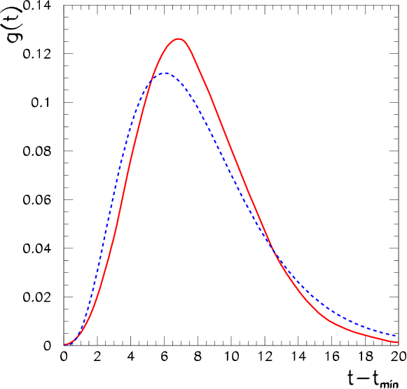
By definition $g(t)$ is a function normalized to $1$ in the interval $t_{\text{min}}\leq t\leq\infty$. With this definition, $t$ would follow a $\chi^{2}$ distribution if $p(\vec{f}|\mathrm{D},L_{\odot})$ were exactly Gaussian. In Fig. 6 we plot the function $g(t)$. For comparison we show the corresponding distribution for a $\chi^{2}$ p.d.f. with 8 degrees of freedom (dashed line).

The significance of the agreement between the data and what is expected under the assumption of a given model is quantified in terms of the probability $P^{\text{agr}}$, defined as the probability to find $t$ in the region of equal or larger compatibility with the data than the level of compatibility observed within the given model:

$$P^{\text{agr}}_{\text{GS(AGS)}}=\int_{t_{\text{GS(AGS)}}}^{t_{\text{max}}}g(t)\,dt$$ (24)

where $t_{\text{GS(AGS)}}$ is the value of the statistic obtained for the central value fluxes of the specific model:

$$t_{\text{GS(AGS)}}=-2\ln\left[p(\vec{\bar{f}}^{\text{GS(AGS)}}|\mathrm{D})\right]\,.$$ (25)

We found that the GS model has a lower $t$, $t_{\text{GS}}=8.5$, while $t_{\text{AGS}}=11.0$. With the probability distribution $g(t)$ shown in Fig. 6 this corresponds to $P^{\text{agr}}_{\text{GS}}=43$% and $P^{\text{agr}}_{\text{AGS}}=20$%.

For comparison we have also constructed a $\chi^{2}$ function comparing the best fit values of the fluxes in each of the models with those obtained in the analysis without the SSM priors and with the uncertainties given by the combined covariance matrix

$$\chi^{2}=\sum_{ij}(\bar{f}^{\text{GS(AGS)}}_{i}-\bar{f}^{\mathrm{D}}_{i})\left[V_{\text{GS(AGS)}}+V_{\mathrm{D}}\right]^{-1}_{ij}(\bar{f}^{\text{GS(AGS)}}_{j}-\bar{f}^{\mathrm{D}}_{j})\,.$$ (26)

Here $V_{\mathrm{D}}$ is the covariance matrix obtained by the best Gaussian approximation to the $p(f_{i}|\mathrm{D},L_{\odot})$ probability distribution function, Eq. (15), and $\bar{f}^{\mathrm{D}}_{j}$ are the best fit fluxes from the data analysis without any SSM prior, Eq. (14). If the distribution $p(\vec{f}|\mathrm{D},L_{\odot})$ were exactly Gaussian, both tests would be equivalent. We found that this test still yields a better fit for the GS model, $\chi^{2}_{\text{GS}}=5.2$ ($P^{\text{agr}}_{\text{GS}}=74\%$) and $\chi^{2}_{\text{AGS}}=5.7$ ($P^{\text{agr}}_{\text{AGS}}=68\%$), but gives a higher probability for both models. We also find that if the prior in Eq. (8) is centered at the BPS08(AGS) prediction the analysis renders the same probability for both models. Conversely if Eq. (8) is centered at the BPS08(GS) prediction the slight preference for the BPS08(GS) model found above is enhanced to $\chi^{2}_{\text{GS}}=5.2$ ($P^{\text{agr}}_{\text{GS}}=74\%$) versus $\chi^{2}_{\text{AGS}}=7.4$ ($P^{\text{agr}}_{\text{AGS}}=50\%$).

From these results we conclude that, while the fit shows a slightly better agreement with the GS model corresponding to higher metallicities, the difference between the two is not statistically significant. This is partly due to the lack of precision of present data. But we also notice that, while the measurements of SNO and SK favor a lower $\mbox{}^{8}\text{B}$ flux as predicted by the low metallicity models, the determination of the $\mbox{}^{7}\text{Be}$ flux in Borexino and the corresponding determination of the pp flux from the luminosity constraint show better agreement with the GS predictions.

4 Summary

We have performed a solar model independent analysis of the solar and terrestrial neutrino data in the framework of three-neutrino oscillations, following a Bayesian approach in terms of a Markov Chain Monte Carlo using the Metropolis-Hastings algorithm. This approach has allowed us to reconstruct the probability distribution function in the entire eleven-dimensional parameter space, consistently incorporating the required set of theoretical priors. The best fit values and allowed ranges for the eight solar neutrino fluxes are summarized in Eq. (14) and Fig. 1 for the analysis with the luminosity constraint, and in Eq. (17) and Fig. 3 for the more general case of unconstrained solar luminosity. We found that at present the neutrino-inferred luminosity perfectly agrees with the measured one and it is known with a $1\sigma$ uncertainty of 14%. We have also tested the fractional energy production in the pp-chain and the CNO-cycle, finding that the total amount of the solar luminosity produced in the CNO-cycle is bounded to be $L_{\text{CNO}}/L_{\odot}<2.8\%$ at 99% CL irrespective of whether the luminosity constraint is imposed or not.

We have then presented a statistical test which can be performed with these results in order to shed some light on the so-called solar composition problem, which at present arises in the construction of the Standard Solar Model. We found that the low value of the $\mbox{}^{8}\text{B}$ flux measured at SK and SNO points towards low metallicity models, whereas the measurement of $\mbox{}^{7}\text{Be}$ in Borexino and the corresponding value of the pp flux implied by the luminosity constraint show better agreement with high metallicity models. Altogether the fit shows a slight preference for models with higher metallicities, however the difference between the two models is not very significant at statistical level. While a realistic improvement of the Borexino data analysis in the near future can positively affect the direct determination of most solar neutrino fluxes, it is unlikely that enough precision will be achieved to go beyond the the present theoretical uncertainties of the SSM’s. The largest difference between the models lies on the CNO fluxes that give predictions which differ by about 30%. Thus ideally in order to achieve a statistically meaningful discrimination between the models one would need a low energy solar neutrino experiment capable of measuring the neutrino energy spectrum for energies between $0.5~{}\text{MeV}\lesssim E_{\nu}\lesssim 1.5~{}\text{MeV}$ and, more importantly, of rejecting the radioactive backgrounds to the required level, so to allow for a determination of the CNO fluxes at $\mathcal{O}(\text{30\%})$ precision.

Appendix A Analysis of Borexino spectra

In our analysis of Borexino we include both the low-energy (LE) data presented in Ref. [40], which are crucial for the reconstruction of the $\mbox{}^{7}\text{Be}$ line, as well as the high-energy (HE) data discussed in Ref. [38], which are mostly sensitive to the $\mbox{}^{8}\text{B}$ flux. For the low-energy part we extracted the 180 experimental data points and the corresponding statistical uncertainties from Fig. 2 of Ref. [40], checking explicitly that the statistical error $\sigma_{b}^{\text{stat}}$ is just the square root of the number of events $N_{b}^{\text{ex}}$ in each bin $b$ (except in the region where statistical $\alpha$’s subtraction had been performed). Similarly, for the high-energy part we extracted the 6 experimental data points and statistical uncertainties from Fig. 3 of Ref. [38]. For both data sets the theoretical prediction $N_{b}^{\text{th}}$ for the bin $b$ is calculated as follows:

$$N_{b}^{\text{th}}(\vec{\omega},\vec{\xi})=n_{\text{el}}T_{b}^{\text{run}}\sum_{\alpha}\int\frac{d\Phi_{\alpha}^{\text{det}}}{dE_{\nu}}(E_{\nu}|\vec{\omega})\,\frac{d\sigma_{\alpha}}{dT_{e}}(E_{\nu},T_{e})\,R_{b}(T_{e}|\vec{\xi})\,dE_{\nu}+N_{b}^{\text{bkg}}(\vec{\xi})$$ (27)

where $\vec{\omega}$ describes both the neutrino oscillation parameters and the eight solar flux normalizations, and $\vec{\xi}$ is a set of variables parametrizing the systematic uncertainties as required by the “pulls” approach to $\chi^{2}$ calculation. Here $n_{\text{el}}$ is the number of electron targets in a fiducial mass of $78.5$ tons with an electron/nucleon ratio of $11/20$ for pseudocumene, and $T_{b}^{\text{run}}$ is the total data-taking time which we set to 192 and 246 live days for LE and HE data, respectively. In the previous formula $d\sigma_{\alpha}/dT_{e}$ is the elastic scattering differential cross-section for neutrinos of type $\alpha\in\{e,\mu,\tau\}$, and $d\Phi_{\alpha}^{\text{det}}/{dE_{\nu}}$ is the corresponding flux of solar neutrinos at the detector – hence it incorporates the neutrino oscillation probabilities. The detector response function $R_{b}(T_{e}|\vec{\xi})$ depends on the true electron kinetic energy $T_{e}$ and on the three systematic variables $\xi_{\text{vol}}$, $\xi_{\text{scl}}$ and $\xi_{\text{res}}$:

$$R_{b}(T_{e}|\vec{\xi})=(1+\pi_{\text{vol}}\,\xi_{\text{vol}})\int_{T_{b}^{\text{min}}(1+\pi^{b}_{\text{scl}}\,\xi_{\text{scl}})}^{T_{b}^{\text{max}}(1+\pi^{b}_{\text{scl}}\,\xi_{\text{scl}})}\mathop{\mathrm{Gauss}}\left[T_{e}-T^{\prime},\,\sigma_{T}(1+\pi_{\text{res}}\,\xi_{\text{res}})\right]\,dT^{\prime}$$ (28)

where $\mathop{\mathrm{Gauss}}(x,\sigma)\equiv\exp\left[-x^{2}/2\sigma^{2}\right]/\sqrt{2\pi}\sigma$ is the normal distribution function, while $T_{b}^{\text{min}}$ and $T_{b}^{\text{max}}$ are the boundaries of the reconstructed electron kinetic energy $T^{\prime}$ in the bin $b$. Note that we assumed an energy resolution $\sigma_{T}/T_{e}=6\%/\sqrt{T_{e}\,\text{[MeV]}}$, rather than the “official” value $5\%\big{/}\sqrt{T_{e}\,\text{[MeV]}}$ quoted by the collaboration, since our choice lead to a perfect match of the $\mbox{}^{7}\text{Be}$ line shown in Fig. 2 of Ref. [40]. We verified that also the other solar fluxes plotted in Ref. [50] are carefully reproduced. As for the effects introduced by systematic uncertainties, we assumed $\pi_{\text{vol}}=6\%$ for the fiducial mass ratio uncertainty, $\pi^{b}_{\text{scl}}=2.4\%$ ($1\%)$ for the energy scale uncertainty in LE (HE) data, and an arbitrary $\pi_{\text{res}}=10\%$ for the energy resolution uncertainty.

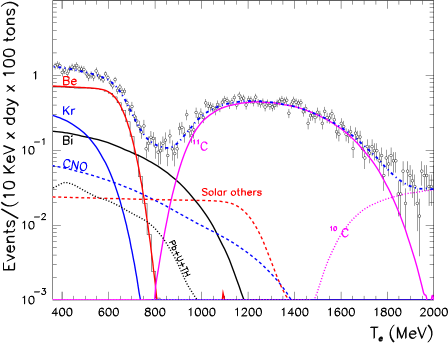
The backgrounds $N_{b}^{\text{bkg}}(\vec{\xi})$ which appear in Eq. (27) only affect the low-energy data, and are not included in the calculation of the high-energy event rates. The $\mbox{}^{10}\text{C}$, $\mbox{}^{11}\text{C}$, $\mbox{}^{14}\text{C}$ and $\mbox{}^{85}\text{Kr}$ background shapes were taken from Fig. 2 of Ref. [40], whereas the $\mbox{}^{238}\text{U}$, $\mbox{}^{214}\text{Pb}$ and $\mbox{}^{210}\text{Bi}$ were extracted from slide 7 of Ref. [50]. We explicitly verified that with the normalizations as inferred from these figures the sum of all these backgrounds with the expected SSM fluxes precisely reproduces the “Fit” line shown in Fig. 2 of Ref. [40]. Note that, because of the overwhelming ${\mbox{}^{14}\text{C}}$ at energies below $\sim 250$ keV, our fit in this energy region is never good. We do not know if this is due to the loss of numerical precision in our extraction of the $\mbox{}^{14}\text{C}$ shape or to the fact that there are additional free parameters to be fitted for this background. In any case, in order to avoid biasing our analysis by the low quality description on these data points we use only the 160 points of the spectrum above $365$ keV. Hence the $\mbox{}^{14}\text{C}$ background is irrelevant. Following the procedure outlined in Ref. [40] the normalization of the $\mbox{}^{238}\text{U}$ and $\mbox{}^{214}\text{Pb}$ backgrounds are assumed to be known, whereas the normalizations of the $\mbox{}^{85}\text{Kr}$, $\mbox{}^{210}\text{Bi}$, $\mbox{}^{11}\text{C}$ and $\mbox{}^{10}\text{C}$ backgrounds are introduced as free parameters and fitted against the data – taking care to ensure their positivity. Hence:

$$N_{b}^{\text{bkg}}(\vec{\xi})=N_{b}^{\text{U238}}+N_{b}^{\text{Pb214}}+N_{b}^{\text{Kr85}}\xi_{\text{Kr85}}+N_{b}^{\text{Bi210}}\xi_{\text{Bi210}}+N_{b}^{\text{C11}}\xi_{\text{C11}}+N_{b}^{\text{C10}}\xi_{\text{C10}}\,.$$ (29)

Figure 7: Spectrum for the best fit point of our spectral fit to the Borexino-LE data in the energy region between 350–2000 KeV under the assumptions described in the Appendix (left) and $\Delta\chi^{2}$ as a function of the $\mbox{}^{7}\text{Be}$ flux for the different test analysis of Borexino data (right).

The $\chi^{2}(\vec{\omega})$ function is constructed in the usual way in the context of the pull method, by introducing standard penalties for the $\vec{\xi}$ variables (except for those parametrizing the free normalizations of the backgrounds) and marginalizing over them:

$$\chi^{2}(\vec{\omega})=\min_{\vec{\xi}}\left\{\sum_{b}\left[\frac{N_{b}^{\text{th}}(\vec{\omega},\vec{\xi})-N_{b}^{\text{ex}}}{\sigma_{b}^{\text{stat}}}\right]^{2}+\xi_{\text{vol}}^{2}+\xi_{\text{scl}}^{2}+\xi_{\text{res}}^{2}\right\}\,.$$ (30)

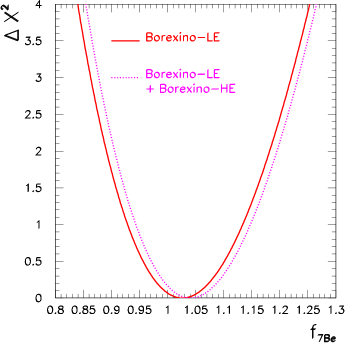
As a test of our procedure we first perform a fit under the same assumptions as Ref. [40], i.e., besides the backgrounds we only fit the $\mbox{}^{7}\text{Be}$ flux normalization to the data. The other solar fluxes are fixed to their BPS08(GS) prediction and the oscillation parameters are fixed to the best fit point of the global pre-Borexino analysis. The results of this test are shown in Fig. 7. Comparing the left panel with Fig. 2 of Ref. [40] we observe a perfect agreement in the best fit $\mbox{}^{7}\text{Be}$ flux spectra. In the right panel we plot the $\Delta\chi^{2}$ for this test fit as a function of $f_{{\mbox{}^{7}\text{Be}}}$, for both Borexino-LE alone and the combination of Borexino-LE and Borexino-HE data. As can be seen, for Borexino-LE our procedure leads to a determination of the $\mbox{}^{7}\text{Be}$ normalization in very good agreement with the value $f_{{\mbox{}^{7}\text{Be}}}=1.02\pm 0.10$ obtained by the Borexino collaboration. The inclusion of the Borexino-HE tends to push the extracted value of $f_{{\mbox{}^{7}\text{Be}}}$ towards a slightly higher value. This is due to the assumed correlation of the systematic uncertainties (in particular the one associated with the total fiducial volume) between LE and the HE. This small effect is diluted once both data sets are included in the global fit, and the final results are practically independent of the degree of correlation assumed between the systematic errors.

Appendix B Details of the Markov Chain Monte Carlo

In this analysis we have used the Metropolis-Hasting algorithm including an adapting algorithm for the kernel function to increase the efficiency. The algorithm is defined as follows:

1. Given a parameter set $\vec{\omega}$, a new value $\vec{\omega}^{\prime}$ is generated according to a transition kernel $q(\vec{\omega},\vec{\omega}^{\prime})$. We start with a flat kernel and, once the chain has reached a certain size, we use a kernel in terms of the covariance matrix $V$ computed with the points in the chain. If $U$ is the matrix diagonalizing $V$ and $d_{i}$ are the eigenvalues, $\vec{\omega}^{\prime}=\vec{\omega}+U\,\vec{\tilde{\omega}}$ with $\tilde{\omega}_{i}$ generated according to a distribution $|\tilde{\omega}_{i}|/d_{i}\times\exp(-\tilde{\omega}_{i}/d_{i})$. The kernel is adapted, i.e., the covariance matrix is recalculated, every several steps.

2. With $\vec{\omega}$ and $\vec{\omega}^{\prime}$ we compute the value:

   $$h=\min\left(1,\frac{\mathcal{L}(\mathrm{D}|\vec{\omega}^{\prime})\,\pi(\vec{\omega}^{\prime}|\mathcal{P})}{\mathcal{L}(\mathrm{D}|\vec{\omega})\,\pi(\vec{\omega}|\mathcal{P})}\right)\,.$$ (31)

3. A random number $0\leq r\leq 1$ is generated and if $r\leq h$, $\vec{\omega}^{\prime}$ is accepted in the chain.

4. We go back to step (1), starting with $\vec{\omega}^{\prime}$ if it has been accepted or again with $\vec{\omega}$ if not.

All the points accepted in this algorithm constitute the Markov Monte-Carlo Chain $\{\vec{\omega}_{\alpha}\}$ with $\alpha=1,\dots,N_{\text{tot}}$, where $N_{\text{tot}}$ is the total number of points in the chain. The method ensures that, once convergence has been reached, the chain takes values over the parameter space with frequency proportional to the posterior probability distribution function.

Technically, in order to reconstruct the posterior p.d.f. from the chain we discretize the parameter space by dividing the physically relevant range of each parameter $\omega_{i}$ into $n_{i}$ subdivisions $\Delta_{i}^{k_{i}}$ of length $\ell^{k_{i}}_{i}$ (with $1\leq k_{i}<n_{i}$). Denoting as $\Omega_{k_{1}\dots k_{m}}$ the cell corresponding to subdivisions $\Delta_{1}^{k_{1}}\dots\Delta_{m}^{k_{m}}$ ($m=10$ or $11$ for the analysis with or without the luminosity constraint, respectively), we compute the value of the posterior p.d.f. as

$$p(\vec{\omega}\in\Omega_{k_{1}\dots k_{m}}|\mathrm{D},\mathcal{P})=\frac{1}{V_{k_{1}\dots k_{m}}}\,\frac{M_{k_{1}\dots k_{m}}}{N_{\text{tot}}}$$ (32)

where $M_{k_{1}\dots k_{m}}$ is the number of points in the chain with parameter values within the cell $\Omega_{k_{1}\dots k_{m}}$, and $V_{k_{1}\dots k_{m}}=\ell^{k_{1}}_{1}\times\dots\times\ell^{k_{m}}_{m}$ is the volume of the cell. In order to ensure that the procedure generates a smooth p.d.f., a sufficiently large $N_{\text{tot}}$ is needed.

The marginalized one-dimensional p.d.f. for the parameter $\omega_{i}$ is reconstructed as

$$p(\omega_{i}\in\Delta_{i}^{k_{i}}|\mathrm{D},\mathcal{P})_{\text{1-dim}}=\frac{1}{\ell^{k_{i}}_{i}}\sum_{{k_{j\neq i}}=1}^{n_{j}}\frac{M_{k_{1}\dots k_{i}\dots k_{m}}}{N_{\text{tot}}}\,.$$ (33)

Similarly, the marginalized two-dimensional p.d.f.’s for the parameters $(\omega_{i},\omega_{j})$ is

$$p(\omega_{i}\in\Delta_{i}^{k_{i}},\omega_{j}\in\Delta_{j}^{k_{j}}|\mathrm{D},\mathcal{P})_{\text{2-dim}}=\frac{1}{\ell^{k_{i}}_{i}\ell^{k_{j}}_{j}}\sum_{{k_{l\neq i,j}}=1}^{n_{l}}\frac{M_{k_{1}\dots k_{i}\dots k_{j}\dots k_{m}}}{N_{\text{tot}}}\,.$$ (34)

From these, we obtain the two-dimensional credibility regions with a given CL as the region with smallest area and with CL integral posterior probability. In practice they are obtained as the regions surrounded by a two-dimensional isoprobability contour which contains the point of highest posterior probability and within which the integral posterior probability is CL.

References

- [1] H. A. Bethe, Energy production in stars, Phys. Rev. 55 (1939) 434–456.
- [2] J. N. Bahcall, Neutrino astrophysics, . Cambridge, UK: University press, 567p.
- [3] J. N. Bahcall and R. K. Ulrich, Solar models, neutrino experiments and helioseismology, Rev. Mod. Phys. 60 (1988) 297–372.
- [4] S. Turck-Chieze, S. Cahen, M. Casse, and C. Doom, Revisiting the standard solar model, Astrophys. J. 335 (1988) 415–424.
- [5] J. N. Bahcall and M. H. Pinsonneault, Standard solar models, with and without helium diffusion and the solar neutrino problem, Rev. Mod. Phys. 64 (1992) 885–926.
- [6] J. N. Bahcall and M. H. Pinsonneault, Solar models with helium and heavy element diffusion, Rev. Mod. Phys. 67 (1995) 781–808, [hep-ph/9505425].
- [7] J. N. Bahcall, M. H. Pinsonneault, and S. Basu, Solar models: Current epoch and time dependences, neutrinos, and helioseismological properties, Astrophys. J. 555 (2001) 990–1012, [astro-ph/0010346].
- [8] J. N. Bahcall, A. M. Serenelli, and S. Basu, New solar opacities, abundances, helioseismology, and neutrino fluxes, Astrophys. J. 621 (2005) L85–L88, [astro-ph/0412440].
- [9] C. Pena-Garay and A. Serenelli, Solar neutrinos and the solar composition problem, arXiv:0811.2424.
- [10] J. N. Bahcall, Solar neutrinos. I: Theoretical, Phys. Rev. Lett. 12 (1964) 300–302.
- [11] J. N. Bahcall, N. A. Bahcall, and G. Shaviv, Present status of the theoretical predictions for the Cl- 36 solar neutrino experiment, Phys. Rev. Lett. 20 (1968) 1209–1212.
- [12] J. N. Bahcall and R. Davis, Solar neutrinos: a scientific puzzle, Science 191 (1976) 264–267.
- [13] B. Pontecorvo, Neutrino experiments and the question of leptonic-charge conservation, Sov. Phys. JETP 26 (1968) 984–988.
- [14] V. N. Gribov and B. Pontecorvo, Neutrino astronomy and lepton charge, Phys. Lett. B28 (1969) 493.
- [15] L. Wolfenstein, Neutrino oscillations in matter, Phys. Rev. D17 (1978) 2369–2374.
- [16] S. P. Mikheev and A. Y. Smirnov, Resonance enhancement of oscillations in matter and solar neutrino spectroscopy, Sov. J. Nucl. Phys. 42 (1985) 913–917.
- [17] M. V. Garzelli and C. Giunti, Model independent information on solar neutrino oscillations, Phys. Rev. D65 (2002) 093005, [hep-ph/0111254].
- [18] J. N. Bahcall, M. C. Gonzalez-Garcia, and C. Pena-Garay, If sterile neutrinos exist, how can one determine the total B-8 and Be-7 solar neutrino fluxes?, Phys. Rev. C66 (2002) 035802, [hep-ph/0204194].
- [19] J. N. Bahcall, M. C. Gonzalez-Garcia, and C. Pena-Garay, Does the sun shine by p p or CNO fusion reactions?, Phys. Rev. Lett. 90 (2003) 131301, [astro-ph/0212331].
- [20] J. N. Bahcall, M. C. Gonzalez-Garcia, and C. Pena-Garay, Solar neutrinos before and after Neutrino 2004, JHEP 08 (2004) 016, [hep-ph/0406294].
- [21] J. N. Bahcall and C. Pena-Garay, Global analyses as a road map to solar neutrino fluxes and oscillation parameters, JHEP 11 (2003) 004, [hep-ph/0305159].
- [22] A. Bandyopadhyay, S. Choubey, S. Goswami, and S. T. Petcov, Solar model parameters and direct measurements of solar neutrino fluxes, Phys. Rev. D75 (2007) 093007, [hep-ph/0608323].
- [23] J. N. Bahcall, S. Basu, M. Pinsonneault, and A. M. Serenelli, Helioseismological implications of recent solar abundance determinations, Astrophys. J. 618 (2005) 1049–1056, [astro-ph/0407060].
- [24] N. Grevesse and A. J. Sauval, Standard solar composition, Space Sci. Rev. 85 (1998) 161–174.
- [25] M. Asplund, N. Grevesse, and J. Sauval, The solar chemical composition, Nucl. Phys. A777 (2006) 1–4, [astro-ph/0410214].
- [26] M. Asplund, N. Grevesse, A. J. Sauval, and P. Scott, The chemical composition of the Sun, Ann. Rev. Astron. Astrophys. 47 (2009) 481–522, [arXiv:0909.0948].
- [27] W. J. Chaplin et al., Solar heavy element abundance: constraints from frequency separation ratios of low-degree p modes, Astrophys. J. 670 (2007) 872–884, [arXiv:0705.3154].
- [28] S. Basu et al., Solar abundances and helioseismology: fine structure spacings and separation ratios of low-degree p modes, Astrophys. J. 655 (2007) 660–671, [astro-ph/0610052].
- [29] A. Serenelli, S. Basu, J. W. Ferguson, and M. Asplund, New solar composition: the problem with solar models revisited, arXiv:0909.2668.
- [30] J. N. Bahcall, The luminosity constraint on solar neutrino fluxes, Phys. Rev. C65 (2002) 025801, [hep-ph/0108148].
- [31] B. T. Cleveland et al., Measurement of the solar electron neutrino flux with the Homestake chlorine detector, Astrophys. J. 496 (1998) 505–526.
- [32] R. L. Hahn, Radiochemical solar neutrino experiments, ’successful and otherwise’, J. Phys. Conf. Ser. 136 (2008) 022003.
- [33] SAGE Collaboration, J. N. Abdurashitov et al., Measurement of the solar neutrino capture rate with gallium metal. III: Results for the 2002–2007 data-taking period, Phys. Rev. C80 (2009) 015807, [arXiv:0901.2200].
- [34] Super-Kamkiokande Collaboration, J. Hosaka et al., Solar neutrino measurements in Super-Kamiokande-I, Phys. Rev. D73 (2006) 112001, [hep-ex/0508053].
- [35] SNO Collaboration, B. Aharmim et al., Measurement of the and total B-8 solar neutrino fluxes with the Sudbury Neutrino Observatory phase I data set, Phys. Rev. C75 (2007) 045502, [nucl-ex/0610020].
- [36] SNO Collaboration, B. Aharmim et al., Electron energy spectra, fluxes, and day-night asymmetries of B-8 solar neutrinos from the 391-day salt phase SNO data set, Phys. Rev. C72 (2005) 055502, [nucl-ex/0502021].
- [37] SNO Collaboration, B. Aharmim et al., An independent measurement of the total active 8B solar neutrino flux using an array of 3He proportional counters at the Sudbury Neutrino Observatory, Phys. Rev. Lett. 101 (2008) 111301, [arXiv:0806.0989].
- [38] Borexino Collaboration, G. Bellini et al., Measurement of the solar 8B neutrino flux with 246 live days of Borexino and observation of the MSW vacuum-matter transition, arXiv:0808.2868v1.
- [39] SNO Collaboration, B. Aharmim et al., Low energy threshold analysis of the phase I and phase II data sets of the Sudbury Neutrino Observatory, arXiv:0910.2984.
- [40] Borexino Collaboration, C. Arpesella et al., Direct measurement of the Be-7 solar neutrino flux with 192 days of Borexino data, Phys. Rev. Lett. 101 (2008) 091302, [arXiv:0805.3843].
- [41] KamLAND Collaboration, I. Shimizu, KamLAND (anti-neutrino status), J. Phys. Conf. Ser. 120 (2008) 052022.
- [42] M. C. Gonzalez-Garcia and M. Maltoni, Phenomenology with massive neutrinos, Phys. Rept. 460 (2008) 1–129, [arXiv:0704.1800].
- [43] CHOOZ Collaboration, M. Apollonio et al., Limits on neutrino oscillations from the CHOOZ experiment, Phys. Lett. B466 (1999) 415–430, [hep-ex/9907037].
- [44] K2K Collaboration, M. H. Ahn et al., Measurement of neutrino oscillation by the K2K experiment, Phys. Rev. D74 (2006) 072003, [hep-ex/0606032].
- [45] MINOS Collaboration, P. Adamson et al., Measurement of Neutrino Oscillations with the MINOS Detectors in the NuMI Beam, Phys. Rev. Lett. 101 (2008) 131802, [arXiv:0806.2237].
- [46] MINOS Collaboration, P. Adamson et al., Search for muon-neutrino to electron-neutrino transitions in MINOS, Phys. Rev. Lett. 103 (2009) 261802, [arXiv:0909.4996].
- [47] M. C. Gonzalez-Garcia, M. Maltoni, and J. Salvado, Updated global fit to three neutrino mixing: status of the hints of , JHEP 04 (2010) 056, [arXiv:1001.4524].
- [48] J. N. Bahcall and P. I. Krastev, How well do we (and will we) know solar neutrino fluxes and oscillation parameters?, Phys. Rev. D53 (1996) 4211–4225, [hep-ph/9512378].
- [49] M. Spiro and D. Vignaud, Solar model independent neutrino oscillation signals in the forthcoming solar neutrino experiments?, Phys. Lett. B242 (1990) 279–284.
- [50] M. Misiaszek, “Last Borexino result.” Talk given at the 2009 Europhysics Conference on High Energy Physics, Krakow, Poland, July 16–22, 2009.