Fifty Years of Stiffness††thanks: Work developed within the project “Numerical methods and software for differential equations”.
Abstract
The notion of stiffness, which originated in several applications of a different nature, has dominated the activities related to the numerical treatment of differential problems for the last fifty years. Contrary to what usually happens in Mathematics, its definition has been, for a long time, not formally precise (actually, there are too many of them). Again, the needs of applications, especially those arising in the construction of robust and general purpose codes, require nowadays a formally precise definition. In this paper, we review the evolution of such a notion and we also provide a precise definition which encompasses all the previous ones.
Keywords: stiffness, ODE problems, discrete problems, initial value problems, boundary value problems, boundary value methods.
1 Introduction
Frustra fit per plura quod potest per pauciora.
Razor of W. of Ockham, doctor invincibilis.
The struggle generated by the duality short times–long times is at the heart of human culture in almost all its aspects. Here are just a few examples to fix the idea:
-
•
in historiography: Braudel’s distinction among the geographic, social and individual times;111 Moreover, his concept of structure, i.e. events which are able to accelerate the normal flow of time, is also interesting from our point of view, because it somehow recalls the mathematical concept of large variation in small intervals of time (see later).
-
•
in the social sphere: Societies are organized according to three kinds of laws, i.e., codes (regulating short term relations), constitutions (regulating medium terms relations), and ethical laws (long term rules) often not explicitly stated but religiously accepted;
-
•
in the economy sphere: the laws of this part of human activities are partially unknown at the moment. Some models (e.g., the Goodwin model [19]), permits us to say, by taking into account only a few variables, that the main evolution is periodic in time (and then predictable), although we are experiencing an excess of periodicity (chaotic behavior). Nevertheless, some experts claim (see, e.g., [18]) that the problems in the predictability of the economy are mainly due to a sort of gap in passing information from a generation to the next ones, i.e. to the conflict between short time and long time behaviors.222 Even Finance makes the distinction between short time and long time traders.
Considering the importance of this concept, it would have been surprising if the duality “short times–long times” did not appear somewhere in Mathematics. As a matter of fact, this struggle not only appears in our field but it also has a name: stiffness.
Apart from a few early papers [10, 11], there is a general agreement in placing the date of the introduction of such problems in Mathematics to around 1960 [17]. They were the necessities of the applications to draw the attention of the mathematical community towards such problems, as the name itself testifies: “they have been termed stiff since they correspond to tight coupling between the driver and the driven components in servo-mechanism” ([12] quoting from [11]).
Both the number and the type of applications proposing difficult differential problems has increased exponentially in the last fifty years. In the early times, the problems proposed by applications were essentially initial value problems and, consequently, the definition of stiffness was clear enough and shared among the few experts, as the following three examples evidently show:
- D1
-
: Systems containing very fast components as well as very slow components
(Dahlquist [12]). - D2
-
: They represent coupled physical systems having components varying with very different times scales: that is they are systems having some components varying much more rapidly than the others (Liniger [31], translated from French).
- D3
-
: A stiff system is one for which is enormous so that either the stability or the error bound or both can only be assured by unreasonable restrictions on …Enormous means enormous relative to the scale which here is (the integration interval)… (Miranker [32]).
The above definitions are rather informal, certainly very far from the precise definitions we are accustomed to in Mathematics, but, at least, they agree on a crucial point: the relation among stiffness and the appearance of different time-scales in the solutions (see also [24]).
Later on, the necessity to encompass new classes of difficult problems, such as Boundary Value Problems, Oscillating Problems, etc., has led either to weaken the definition or, more often, to define some consequence of the phenomenon instead of defining the phenomenon itself. In Lambert’s book [29] five propositions about stiffness, each of them capturing some important aspects of it, are given. As matter of fact, it has been also stated that no universally accepted definition of stiffness exists [36].
There are, in the literature, other definitions based on other numerical difficulties, such as, for example, large Lipschitz constants or logarithmic norms [37], or non-normality of matrices [23]. Often is not even clear if stiffness refers to particular solutions (see, e.g. [25]) or to problems as a whole.
Sometimes one has the feeling that stiffness is becoming so broad to be nearly synonymous of difficult.
At the moment, even if the old intuitive definition relating stiffness to multiscale problems survives in most of the authors, the most successful definition seems to be the one based on particular effects of the phenomenon rather than on the phenomenon itself, such as, for example, the following almost equivalent items:
- D4
-
: Stiff equations are equations where certain implicit methods …perform better, usually tremendous better, than explicit ones [11].
- D5
-
: Stiff equations are problems for which explicit methods don’t work [21].
- D6
-
: If a numerical method with a finite region of absolute stability, applied to a system with any initial condition, is forced to use in a certain interval of integration a step length which is excessively small in relation to the smoothness of the exact solution in that interval, then the system is said to be stiff in that interval [29].
As usually happens, describing a phenomenon by means of its effects may not be enough to fully characterize the phenomenon itself. For example, saying that fire is what produces ash, would oblige firemen to wait for the end of a fire to see if the ash has been produced. In the same way, in order to recognize stiffness according to the previous definitions, it would be necessary to apply first one333 It is not clear if one is enough: in principle the definition may require to apply all of them. explicit method and see if it works or not. Some authors, probably discouraged by the above defeats in giving a rigorous definition, have also affirmed that a rigorous mathematical definition of stiffness is not possible [20].
It is clear that this situation is unacceptable for at least two reasons:
-
•
it is against the tradition of Mathematics, where objects under study have to be precisely defined;
-
•
it is necessary to have the possibility to recognize operatively this class of problems, in order to increase the efficiency of the numerical codes to be used in applications.
Concerning the first item, our opinion is that, in order to gain in precision, it would be necessary to revise the concept of stability used in Numerical Analysis, which is somehow different from the homonym concept used in all the other fields of Mathematics, where stable are equilibrium points, equilibrium sets, reference solutions, etc., but not equations or problems444 Only in particular circumstances, for example in the linear case, it is sometimes allowed the language abuse: the nonlinear case may contain simultaneously stable and unstable solutions. (see also [17] and [30]).
Concerning the second item, operatively is intended in the sense that the definition must be stated in terms of numerically observable quantities such as, for example, norms of vectors or matrices. It was believed that, seen from the applicative point of view, a formal definition of stiffness would not be strictly necessary: Complete formality here is of little value to the scientist or engineer with a real problem to solve [24].
Nowadays, after the great advance in the quality of numerical codes,555 A great deal of this improvement is due to the author of the previous sentence. the usefulness of a formal definition is strongly recognised, also from the point of view of applications: One of the major difficulties associated with the study of stiff differential systems is that a good mathematical definition of the concept of stiffness does not exist [6].
In this paper, starting from ideas already partially exposed elsewhere [2, 4, 26], we will try to unravel the question of the definition of stiffness and show that a precise and operative definition of it, which encompasses all the known facets, is possible.
In order to be as clear as possible, we shall start with the simpler case of initial value for a single linear equation and gradually we shall consider more general cases and, eventually, we shall synthesize the results.
2 The asymptotic stability case
For initial value problems for ODEs, the concept of stability concerns the behavior of a generic solution , in the neighborhood of a reference solution , when the initial value is perturbed. When the problem is linear and homogeneous, the difference, , satisfies the same equation as . For nonlinear problems, one resorts to the linearized problem, described by the variational equation, which, essentially, provides valuable information only when is asymptotically stable. Such a variational equation can be used to generalize to nonlinear problems the arguments below which, for sake of simplicity, concerns only the linear case.
Originally, stiffness was almost always associated with initial value problems having asymptotically stable equilibrium points (dissipative problems) (see, e.g., Dahlquist [13]). We then start from this case, which is a very special one. Its peculiarities arise from the following two facts:666 We omit, for simplicity, the other fact which could affect new definitions, i.e., the fact that the solutions of the linear equation can be integrated over any large interval because of the equivalence, in this case, between asymptotic and exponential stability.
-
•
it is the most common in applications;
-
•
there exists a powerful and fundamental theorem, usually called Stability in the first approximation Theorem or Poincaré-Liapunov Theorem, along with its corollary due to Perron777 It is interesting to observe that the same theorem is known as the Ostrowsky’s Theorem, in the theory of iterative methods., which allows us to reduce the study of stability of critical points, of a very large class of nonlinearities, to the study of the stability of the corresponding linearized problems (see, e.g., [9, 27, 35, 38]).
The former fact explains the pressure of applications for the treatment of such problems even before the computer age. The latter one provides, although not always explicitly recognized, the mathematical solid bases for the profitable and extensive use, in Numerical Analysis, of the linear test equation to study the fixed- stability of numerical methods.
We shall consider explicitly the case where the linearized problem is autonomous, although the following definitions will take into account the more general case.
Our starting case will then be that of an initial value problem having an asymptotically stable reference solution, whose representative is, in the scalar case,
| (1) | |||||
where the reference solution (an equilibrium point, in this case) has been placed at the origin. From what is said above, it turns out that it is not by chance that it coincides with the famous test equation.
Remark 2.1
It is worth observing that the above test equation is not less general than , which very often appears in the definitions of stiffness: the only difference is the reference solution, which becomes , but not the topology of solutions around it. This can be easily seen by introducing the new variable which satisfies exactly equation (1) and then, trivially, must share the same stiffness. Once the solution of the homogeneous equation has been obtained, the solution is obtained by adding to it which, in principle, could be obtained by means of a quadrature formula. This allows us to conclude that if any stiffness is in the problem, this must reside in the homogeneous part of it, i.e., in problem (1).
Remark 2.2
We call attention to the interval of integration , which depends on our need for information about the solution, even if the latter exists for all values of . This interval must be considered as datum of the problem. This has been sometimes overlooked, thus creating some confusion.
Having fixed problem (1), we now look for a mathematical tool which allows us to state formally the intuitive concept, shared by almost all the definitions of stiffness: i.e., we look for one or two parameters which tells us if in the solution varies rapidly or not. This can be done easily by introducing the following two measures for the solution of problem (1):
| (2) |
which, in the present case, assume the values:
where is the transient time. The two measures , are called conditioning parameters because they measure the sensitivity of the solution subject to a perturbation of the initial conditions in the infinity and in the norm.
Sometimes, it would be preferable to use a lower value of , i.e.,
| (3) |
This amounts to consider also the oscillating part of the solution (see also Remark 2.4 below).
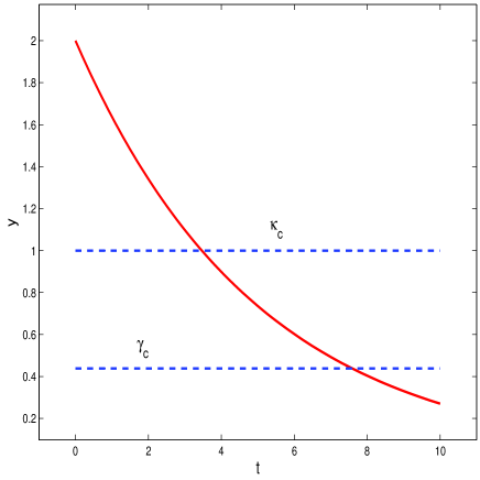
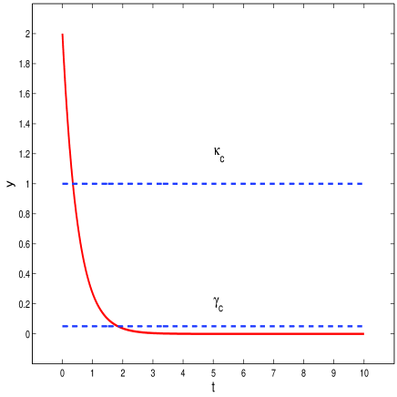
By looking at Figure 1, one realizes at once that a rapid variation of the solution in occurs when It follows then that the parameter
| (4) |
which is the ratio between the two characteristic times of the problem, is more significant. Consequently, the definition of stiffness follows now trivially:
Definition 2.1
The initial value problem (1) is stiff if .
The parameter is called stiffness ratio.
Remark 2.3
The width of the integration interval plays a fundamental role in the definition. This is an important point: some authors, in fact, believe that stiffness should concern equations; some others believe that stiffness should concern problems, i.e., equations and data. We believe that both statements are partially correct: stiffness concerns equations, integration time, and a set of initial data (not a specific one of them). Since this point is more important in the non scalar case, it will be discussed in more detail later.
Remark 2.4
When is defined according to (3), the definition of stiffness continues to be also meaningful in the case , i.e., when the critical point is only marginally stable. In fact, let
Then,
and the definition encompasses also the case of oscillating stiffness introduced by some authors (e.g., [32]). Once again the stiffness is the ratio of two times. If information about the solution on the smaller time scale is needed, an adequately small stepsize should be used. It is worth noting that high oscillating systems (with respect to ) fall in the class of problems for which explicit methods do not work, and then are stiff according to definitions D4–D6.
When , then
In the case (i.e., the case of an unstable critical point), both parameters and grow exponentially with time. This implies that small variations in the initial conditions will imply exponentially large variations in the solutions, both pointwise and on average: i.e., the problem is ill conditioned.
Of course, the case considered above cannot be considered as representative of more difficult nonlinear equations, since linearization is in general not allowed in such a case.
The linearization is not the only way to study nonlinear differential (or difference) equations. The so called Liapunov second method can be used as well (see, e.g., [22, 27, 38]). It has been used, in connection with stiffness in [5, 13, 14, 15, 16, 17], although not always explicitly named.888 Often, it appears under the name of one-sided Lipschitz condition. Anyway, no matter how the asymptotic stability of a reference solution is detected, the parameters (2) and Definition 2.1 continue to be valid. Later on, the problem of effectively estimating such parameters will also be discussed.
2.1 The discrete case
Before passing to the non scalar case, let us now consider the discrete case, where some interesting additional considerations can be made. Here, almost all we have said for the continuous case can be repeated. The first approximation theorem can be stated almost in the same terms as in the continuous case (see e.g. [28]).
Let the interval be partitioned into subintervals of length , thus defining the mesh points:
The linearized autonomous problem is now:
| (5) |
where the are complex parameters. The conditioning parameters for (5), along with the stiffness ratio, are defined as:
| (6) |
This permits us to define the notion of well representation of a continuous problem by means of a discrete one.
In the case of a constant mesh-size , and it easily follows that the condition (7) requires . It is not difficult to recognize the usual -stability conditions for one-step methods (see Table 1). Furthermore, it is easily recognized that the request that condition (7) holds uniformly with respect to implies that the numerical method producing (5) must be implicit.
| method | condition | |
|---|---|---|
| Explicit Euler | ||
| Implicit Euler | ||
| Trapezoidal Rule |
What does condition (8) require more? Of course, it measures how faithfully the integral is approximated by the quadrature formula , thus giving a sort of global information about the behavior of the method producing the approximations . One of the most efficient global strategies for changing the stepsize is based on monitoring this parameter [3, 4, 7, 8, 33, 34]. In addition to this, when finite precision arithmetic is used, then an interesting property of the parameter occurs [26]: if it is smaller than a suitably small threshold, this suggests that we are doing useless computations, since the machine precision has already been reached.
2.2 The non scalar case
In this case, the linearized problem to be considered is
| (9) |
with and having all its eigenvalues with negative real part. It is clear from what was said in the scalar case that, denoting by the fundamental matrix of the above equation, the straightforward generalization of the definition of the conditioning parameters (2) would lead to:
| (10) |
Indeed, these straight definitions work most of the time, as is confirmed by the following example, although, as we shall explain soon, not always.
Example 2.1
Let us consider the well-known Van der Pol’s problem,
| (11) | |||||
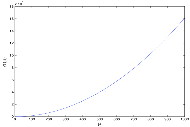
Even though (10) works for this problem, this is not true in general. The problem is that the definition of stiffness as the ratio of two quantities may require a lower bound for the denominator. While the definition of remains unchanged, the definition of is more entangled. Actually, we need two different estimates of such a parameter:
-
•
an upper bound, to be used for estimating the conditioning of the problem in norm;
-
•
a lower bound, to be used in defining and, then, the stiffness.
In the definition given in [2, 4], this distinction was not made, even though the definition was (qualitatively) completed by adding
| “for at least one of the modes”. | (12) |
We shall be more precise in a moment. In the meanwhile, it is interesting to note that the clarification contained in (12) is already in one of the two definitions given by Miranker [32]:
A system of differential equations is said to be stiff on the interval if there exists a solution of that system a component of which has a variation on that interval which is large compared to ,
where it should be stressed that the definition considers equations and not problems: this implies that the existence of largely variable components may appear for at least one choice of the initial conditions, not necessary for a specific one.
Later on, the definition was modified so as to translate into formulas the above quoted sentence (12). The following definitions were then given (see, e.g., [26]):
| (13) |
and
| (14) |
The only major change regards the definition of Let us be more clear on this point with an example, since it leads to a controversial question in the literature: i.e., the dependence of stiffness from the initial condition. Let with and . The solution of problem (9) is .
If is defined according to (10), it turns out that and, then, If, however, we take , then and becomes . Of course, by changing the initial point, one may activate each one of the modes, i.e. the functions on the diagonal of the matrix , leaving silent the others. This is the reason for specifying, in the older definition, the quoted sentence (12). The new definition (14), which essentially poses as the denominator of the ratio the smallest value among the possible values of , is more compact and complies with the needs of people working on the construction of codes, who like more operative definitions. For the previous diagonal example, we have that continues to be equal to 1, while .
Having got the new definition (14) of , the definition of stiffness continues to be given by Definition 2.1 given in the scalar case, i.e., the problem (9) is stiff if .
How does this definition reconcile with the most used definition of stiffness for the linear case, which considers the “smallest” eigenvalue as well? The answer is already in Miranker’s definition D3. In fact, usually the integration interval is chosen large enough to provide complete information on the behavior of the solution. In this case, until the slowest mode has decayed enough, i.e. , which implies
| (15) |
which, when much larger than 1, coincides with the most common definition of stiffness in the linear case. However, let us insist on saying that if the interval of integration is much smaller than , the problem may be not stiff even if .
The controversy about the dependence of the definition of stiffness on the initial data is better understood by considering the following equation given in [29, pp. 217–218]:
whose general solution is
The initial condition requires and, then, the slowest mode is not activated: the solution rapidly reaches the reference solution. If this information was known beforehand, one could, in principle, choose the interval of integration much smaller than . This, however, does not take into account the fact that the computer uses finite precision arithmetic, which may not represent exactly the initial condition . To be more precise, let us point out that the slowest mode is not activated only if the initial condition is on the line . Any irrational value of will not be well represented on the computer. This is enough to activate the silent mode. Of course, if one is sure that the long term contribution to the solution obtained on the computer is due to this kind of error, a small value of can always be used. But it is rare that this information is known in advance. For this reason, we consider the problem to be stiff, since we believe that the definition of stiffness cannot distinguish, for example, between rational and irrational values of the initial conditions. Put differently, initial conditions are like a fuse that may activate stiffness.
We conclude this section by providing a few examples, which show that Definition 2.1, when is defined according to (14), is able to adequately describe the stiffness of nonlinear and/or non autonomous problems as well.
Example 2.2
Let us consider the well-known Robertson’s problem:
| (16) | |||||
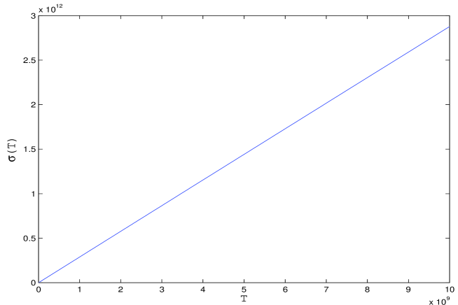
Its stiffness ratio with respect to the length of the integration interval, obtained through the linearized problem and considering a perturbation of the initial condition of the form , is plotted in Figure 3. As it is well-known, the figure confirms that for this problem stiffness increases with .
Example 2.3
Let us consider the so-called Kreiss problem [21, p. 542], a linear and non autonomous problem:
| (17) |
where
| (18) |
and
| (19) |
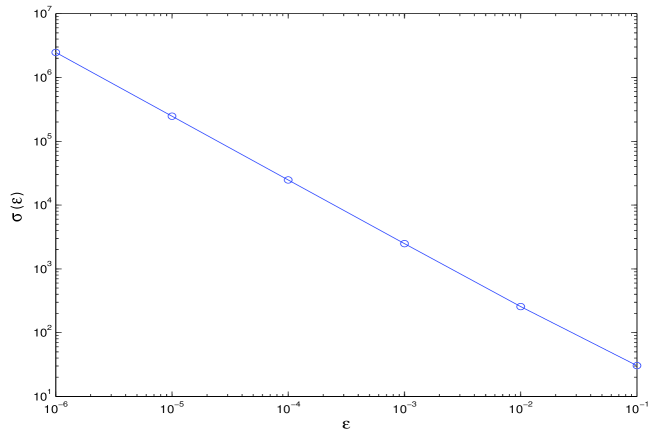
Its stiffness ratio with respect to the small positive parameter , obtained by considering a perturbation of the initial condition of the form , is plotted in Figure 4. As one expects, the figure confirms that the stiffness of the problem behaves as , as tends to 0.
Example 2.4
Let us consider the following linear and non autonomous problem, a modification of problem (17), that we call “modified Kreiss problem”: 999 This problem has been suggested by J.I. Montijano.
| (20) |
where
| (21) |
and
| (22) |
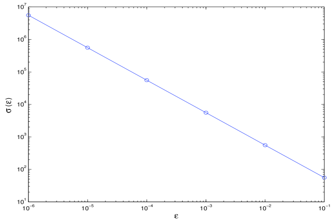
Its stiffness ratio with respect to the small positive parameter , obtained by considering a perturbation of the initial condition of the form , is shown in Figure 5. Also in this case the stiffness of the the problem behaves as , as tends to 0.
Remark 2.5
It is worth mentioning that, in the examples considered above, we numerically found that
is obtained by considering an initial condition in the direction of the eigenvector of the Jacobian matrix (computed for ) associated to the dominant eigenvalue. We note that, for an autonomous linear problem, if is diagonalizable, this choice activates the mode associated with , i.e., the eigenvalue of maximum modulus of .
2.3 The non scalar discrete case
As for the scalar case, what we said for the continuous problems can be repeated, mutatis mutandis, for the discrete ones. For brevity, we shall skip here the details for this case, also because they can be deduced from those described in the more general case discussed in the next section.
3 Boundary Value Problems (BVPs)
The literature about BVPs is far less abundant than that about IVPs, both in the continuous and in the discrete case. While there are countless books on the latter subject presenting it from many points of view (e.g., stability of motion, dynamical systems, bifurcation theory, etc.), there are many less books about the former. More importantly, the subject is usually presented as a by product of the theory of IVPs. This is not necessarily the best way to look at the question, even though many important results can be obtained this way. However, it may sometimes be more useful to look at the subject the other way around. Actually, the question is that IVPs are naturally a subclass of BVPs. Let us informally clarify this point without many technical details which can be found, for example, in [4].
IVPs transmit the initial information “from left to right”. Well conditioned IVPs are those for which the initial value, along with the possible initial errors, decay moving from left to right. FVPs (Final Value problems) are those transmitting information “from right to left” and, of course, well conditioning should hold when the time, or the corresponding independent variable, varies towards . More precisely, considering the scalar test equation (1), the asymptotically stability for IVPs and FVPs requires and , respectively. BVPs transmit information both ways. Consequently, they cannot be scalar problems but vectorial of dimension at least two. We need then to refer to the test equation (9). It can be affirmed that a well conditioned linear BVP needs to have eigenvalues with both negative and positive real parts (dichotomy, see, e.g., [1, 4]). More precisely: the number of eigenvalues with negative real part has to match the amount of information transmitted “from left to right”, and the number of eigenvalues with positive real part has to match the amount of information traveling “from right to left”. For brevity, we shall call the above statement continuous matching rule. Of course, if there are no final conditions, then the problem becomes an IVP and, as we have seen, in order to be well conditioned, it must have all the eigenvalues with negative real part. In other words, the generalization of the case of asymptotically stable IVPs is the class of well conditioned BVPs because both satisfy the continuous matching rule. This is exactly what we shall assume hereafter.
Similar considerations apply to the discrete problems, where the role of the imaginary axis is played by the unit circumference in the complex plane. It is not surprising that a numerical method will well represent a continuous autonomous linear BVP if the corresponding matrix has as many eigenvalues inside the unit circle as the number of initial conditions and as many eigenvalues outside the unit circle as the number of final conditions (discrete matching rule).
Remark 3.1
The idea that IVPs are a subset of BVPs is at the root of the class of methods called Boundary Value Methods (BVMs) which permits us, thanks to the discrete matching rule, to define high order and perfectly -stable methods (i.e., methods having the imaginary axis separating the stable and unstable domains), which overcome the Dahlquist’s barriers, and are able to solve both IVPs and BVPs (see, e.g., [4]).
Remark 3.2
From this point of view, the popular shooting method, consisting of transforming a BVP into an IVP and then applying a good method designed for IVPs, does not appear to be such a good idea. As matter of fact, even a very well conditioned linear BVP, i.e. one which satisfies the continuous matching rule, will be transformed in a badly conditioned IVP, since the matrix of the continuous IVP shall, of course, contain eigenvalues with positive real part. This will prevent the discrete matching rule to hold.
3.1 Stiffness for BVPs
Coming back to our main question, stiffness for BVPs is now defined by generalizing the idea already discussed in the previous sections.
As in the previous cases, we shall refer to linear problems, but the definitions will also be applicable to nonlinear problems as well. Moreover, according to what is stated above, we shall only consider the case where the problems are well conditioned (for the case of ill conditioned problems, the arguments are slightly more entangled, see e.g. [7]). Then, let us consider the linear and non autonomous BVP:
| (23) |
where and . The solution of the problem (23) is
where is the fundamental matrix of the problem such that , and , which has to be nonsingular, in order for (23) to be solvable.101010 Observe that, in the case of IVPs, and , so that .
As in the continuous IVP case, the conditioning parameters are defined (see (13)) as:
Consequently, the stiffness ratio is defined as (see (14)):
and the problem is stiff if . Moreover, upper bounds of and are respectively given by:
| (25) |
Thus, the previous definitions naturally extend to BVPs the results stated for IVPs. In a similar way, when considering the discrete approximation of (23), for the sake of brevity provided by a suitable one-step method over a partition of the interval , with subintervals of length , , the discrete problem will be given by
| (26) |
whose solution is given by
The corresponding discrete conditioning parameters are then defined by:
and
According to Definition 2.2, we say that the discrete problem111111 It is both defined by the used method and by the considered mesh. (26) well represents the continuous problem (23) if
| (28) |
Remark 3.3
3.2 Singular Perturbation Problems
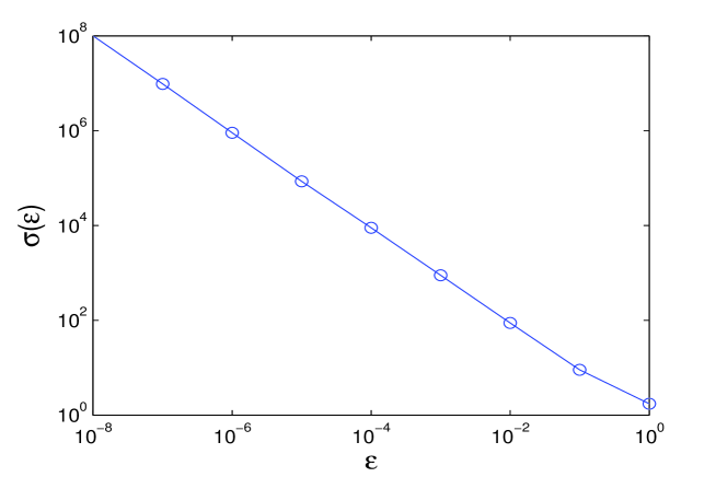
The numerical solution of singular perturbation problems can be very difficult because they can have solutions with very narrow regions of rapid variation characterized by boundary layers, shocks, and interior layers. Usually, the equations depend on a small parameter, say , and the problems become more difficult as tends to 0. It is not always clear, however, how the width of the region of rapid variation is related to the parameter . By computing the stiffness ratio , we observe that singularly perturbed problems are stiff problems. Moreover, as the following examples show, the parameter provides us also with information about the width of the region of rapid variation.
The examples are formulated as second order equations: of course, they have to be transformed into corresponding first order systems, in order to apply the results of the previous statements.
Example 3.1
Let us consider the linear singularly perturbed problem:
| (29) |
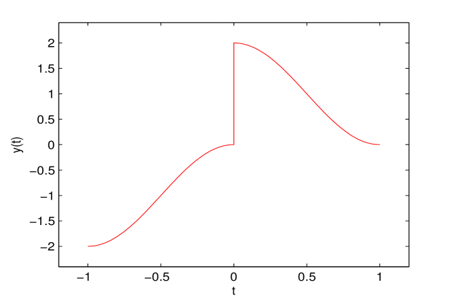
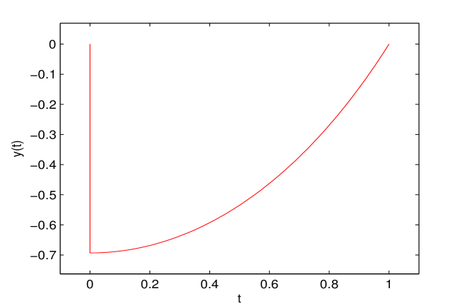
whose solution has, for , a turning point at (see Figure 6). The exact solution is
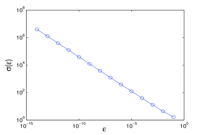
In Figure 7 we plot an estimate of the stiffness ratio obtained by considering two different perturbations of the boundary conditions of the form and . The parameter varies from to . We see that the (estimated) stiffness parameter grows like .
Example 3.2
Let us consider the following nonlinear problem:
| (30) |
This problem has a boundary layer at (see Figure 8). In Figure 9 we plot an estimate of the stiffness ratio obtained by considering two different perturbations of the boundary conditions of the form and . The parameter varies from to . We see that the (estimated) stiffness parameter grows like , as tends to 0.
Example 3.3
Let us consider the nonlinear Troesch problem:
| (31) |
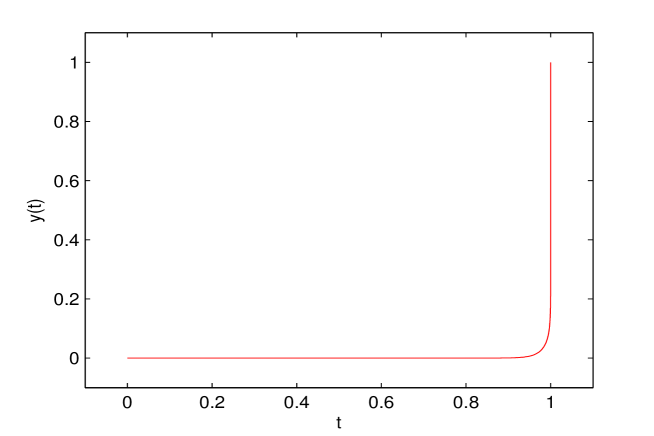
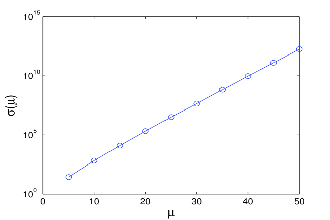
This problem has a boundary layer near (see Figure 10). In Figure 11 we plot the estimate of the stiffness ratio obtained by considering two different perturbations of the boundary conditions of the form and . The parameter is increased from 1 to 50 and, as expected, the stiffness ratio increases as well: for , it reaches the value .
Acknowledgements
The authors wish to thank the reviewers, for their comments and suggestions.
References
- [1] U.M. Ascher, R.M.M. Mattheij, R.D. Russell. Numerical Solution of Boundary Value Problems for Ordinary Differential Equations, SIAM, Philadelphia, 1995.
- [2] L. Brugnano, D. Trigiante, On the characterization of stiffness for ODEs. Dynamics of Continuous, Discrete and Impulsive Systems 2 (1996) 317–335.
- [3] L. Brugnano, D. Trigiante. A new mesh selection strategy for ODEs. Appl. Numer. Math. 24 (1997) 1–21.
- [4] L. Brugnano, D. Trigiante. Solving Differential Problems by Multistep Initial and Boundary Value Methods. Gordon & Breach, Amsterdam, 1998.
- [5] J.C. Butcher. The Numerical Analysis of Ordinary Differential Equations. John Wiley, Chichester, 1987.
- [6] J.R. Cash. Efficient Numerical Methods for the Solution of Stiff Initial-value Problems and Differential Algebraic Equations. Proc. R. Soc. Lond. A 459 (2003) 797–815.
- [7] J.R. Cash, F. Mazzia. A new mesh selection algorithm, based on conditioning, for two-point boundary value codes. J. Comput. Appl. Math. 184 (2005) 362–381.
- [8] J.R. Cash, N. Sumarti, F. Mazzia, D. Trigiante. The Role of Conditioning in Mesh Selection Algorithms for First Order Systems of Linear Two-Point Boundary Value Problems. Journal of Computational and Applied Mathematics 185 (2006) 212–224
- [9] C. Corduneanu. Principles of Differential and Integral Equations. Chelsea, New York, 1971.
- [10] J. Crank, P. Nicolson. A Pratical Method for Numerical Evaluation of Solutions od Partial Differential Equations of the Heat-conduction Type. Proc. Camb. Phil. Soc. 43 (1947) 50–67.
- [11] G.F. Curtiss, J.O. Hirshfelder. Integration of Stiff Equations. Proc. Nat. Acad. Science U.S. 38 (1952) 235–243.
- [12] G. Dahlquist. Problems Related to the Numerical Treatment of Stiff Differential Equations. In E. Günther et al. International Computing Symposium (1973). North Holland, 1974, pp. 307–314.
- [13] G. Dahlquist. A Special Stability Problem for Linear Multistep Methods. BIT 3 (1964) 27–43.
- [14] G. Dahlquist. Error analysis for a class a methods for stiff nonlinear initial value problems. Num. Anal., Dundee, Lect. Notes in Math. 506 (1975) 60–74.
- [15] G. Dahlquist. On stability and error analysis for stiff nonlinear problems. Part 1. Report Trita-NA-7508 (1975).
- [16] G. Dahlquist. -stability is equivalent to -stability. BIT 18 (1978) 384–401.
- [17] G. Dahlquist. 33 Years of Instability, Part I. BIT 25 (1985) 188–204.
- [18] J.K. Galbraith. A Short History of Financial Euphoria. Whittle Direct Book, 1990.
- [19] R.H. Goodwin. A Growth Cycle. In “Socialism, Capitalism and Economic Growth”, C.H. Feinstein Ed., Cambridge University Press, 1967.
- [20] N. Guglielmi and E. Hairer (2007), Stiff delay equations, Scholarpedia, 2(11):2850.
- [21] E. Hairer, G. Wanner. Solving Ordinary Differential Equations II, 2nd rev. ed., Springer-Verlag, Berlin, 1996.
- [22] W. Hahn. Stability of Motions. Springer-Verlag, New York, 1967.
- [23] D.J. Higham, L.N. Trefethen. Stiffness of ODE. BIT 33 (1993) 286–303.
- [24] A.C. Hindmarsh. On Numerical Methods for Stiff Differential Equations–Getting the Power to the People. Lawrence Livermore Laboratory report, UCRL-83259 (1979).
- [25] W.H. Hundsdorfer. The numerical solution of stiff initial value problems: an analysis of one step methods. CWI Tracts 12, Amsterdam, 1980.
- [26] F. Iavernaro, F. Mazzia, D. Trigiante. Stability and conditioning in Numerical Analysis. JNAIAM 1 (2006) 91–112.
- [27] V. Lakshmikantham, S. Leela. Differential and Integral Inequalities. Academic Press, New York, 1969.
- [28] V. Lakshikantham, D. Trigiante. Theory of Difference Equations. Numerical Methods and Applications. Second Edition. Marcel Dekker, New York, 2002.
- [29] J.D. Lambert. Numerical Methods for Ordinary Differential Equations. John Wiley, New York, 1991.
- [30] R.J. Le Veque. Finite Difference Methods for Ordinary and Partial Differential Equations: Steady-State and Time-Dependent Problems. SIAM, Philadelphia, 2007.
- [31] W. Liniger. Solution Numériques des Équations Différentielle et au derivées partielle. Unpublished Lecture Notes of a course taught at Swiss Federal Institute of Technology, Lausanne, Switzerland, 1972–1973.
- [32] W.L. Miranker. The Computational Theory of Stiff Differential Equations. Pubblicazioni IAC Roma Ser. III N. 102, 1975.
- [33] F. Mazzia, D. Trigiante. A hybrid mesh selection strategy based on conditioning for boundary value ODEs problems. Numerical Algorithms 36(2) (2004) 169–187.
- [34] F. Mazzia, D. Trigiante, Efficient Strategies for Solving Nonlinear Problems in BVPs Codes. Nonlinear Studies (in press).
- [35] N. Rouche, J. Mawhin. Équations differentielle Ordinaire. Tome 2. Masson et Cie, Paris, 1973.
- [36] L.F. Shampine and S. Thompson (2007), Stiff Systems, Scholarpedia, 2(3):2855.
- [37] G. Söderlind. The Logarithmic Norm. History and Modern Theory. BIT 46 (2006) 631–652.
- [38] T. Yoshizawa. Stability Theory by Liapunov’s Second Method. The Mathematical Soc. of Japan, 1966.