Multiplicity fluctuations and temperature fluctuations

Abstract

We argue that specific fluctuations observed in high-energy nuclear collisions can be attributed to intrinsic fluctuations of temperature of the hadronizing system formed in such processes and therefore can be described by the same nonextensivity parameter $q$ characterizing Tsallis statistics describing such systems (for $q\rightarrow 1$ one recovers the usual Boltzmann-Gibbs approach). It means that $|q-1|$, which is a direct measure of temperature fluctuations, can also be expressed by the observed mean multiplicity, $\langle N\rangle$, and by its variance, $Var(N)$. This allows to deduce from the experimental data the system size dependence of parameter $q$ with $q=1$ corresponding to an infinite, thermalized source with a fixed temperature, and with the observed $q>1$ corresponding to a finite source in which both the temperature and energy fluctuate.

Since already some time we advocate that most of the single particle distributions measured in high energy collisions when analyzed by statistical hadronization model should use its nonextensive version (for all details concerning nonextensive statistical physics and its applications see recent review T , our works are summarized there in EPJA ). In such approach a standard Boltzmann-Gibbs (BG) exponential distributions, $g(E)=C\exp(-E/T)$, are replaced by Tsallis distribution ($q$-exponential), $h_{q}(E)=C_{q}\left[1-(1-q)E/T\right]^{1/(1-q)}$, and a new phenomenological parameter $q$ occurs which accounts summarily for the possible intrinsic fluctuations of the usual parameter, the temperature $T$ of the hadronizing system, $q-1=Var(T)/\langle T\rangle^{2}$ (for $q\rightarrow 1$ one recovers the usual BG approach). Because $Var(T)/\langle T\rangle^{2}=1/C_{V}$ ($C_{V}$ is the heat capacity under constant volume) it means that $q-1=1/C_{V}$ in fact measures the heat capacity of hadronizing system. In nuclear collisions in which only part of nucleus participates actively in the collision, the above picture should be slightly modified by allowing for the energy transfer to/from the collision region to its surroundings (formed by the spectator nucleons), As result $T$ in the above formulas is replaced by $T_{eff}=T_{0}+(q-1)T_{visc}$, with $T_{0}=\langle T\rangle$ and $T_{visc}$ being a new parameter characterizing this energy transfer EPJA ; OurPaper . On the other hand, it was also shown in EPJA that whereas independently produced particles following BG distributions in energy show Poisson multiplicity distributions, the same particles following Tsallis distributions instead are inevitably distributed according to the Negative Binomial formula, $P(N)=\Gamma(N+k)/\left[\Gamma(N+1)\Gamma(k)\right]=\left(\langle N\rangle\right)^{N}/\left(1+\langle N\rangle/k\right)^{N+1}$ with $k=1/(q-1)$ (or $q=1+1/k$) and $Var(N)=\langle N\rangle+(q-1)\langle N\rangle^{2}$.

Let us now observe that for a system with finite size remaining in contact with a heat bath one has, following Lindhard’s approach Lin , that

$$Var(U)+C_{V}^{2}Var(T)=\langle T\rangle^{2}C_{V}.$$ (1)

This is a kind of uncertainty relation (in the sense that it expresses the truth that in the case of conjugate variables one standard deviation in some measurement can only become small at the expense of the increase of some other standard deviation UnRel ). Relation (1) is supposed to be valid all the way from the canonical ensemble,

$$Var(T)=0\quad{\rm and}\quad Var(U)=\langle T\rangle^{2}C_{V},$$ (2)

to the microcanonical ensemble,

$$Var(T)=\langle T\rangle^{2}/C_{V}\quad{\rm and}\quad Var(U)=0.$$ (3)

It means therefore that Eq. (1) expresses both the complementarity between the temperature and energy, and between the canonical and microcanonical description of the system. This should be understood in the same way as the (improper) eigenstates of position and momentum appear as extreme cases in the quantum mechanical uncertainty relations. It is worth knowing that in limq the limiting cases of Tsallis statistics was investigated in which $q$ was interpreted as a measure thermal bath heat capacity: $q=1$, i.e. canonical, case would correspond to an infinite bath (thermalized and with fixed temperature), whereas $q=-\infty$, i.e. microcanonical, case would correspond to a bath with null heat capacity (isolated and with fixed energy). All intermediate cases would then correspond to the finite heat capacity (both temperature and energy fluctuate).

To obtain realistic (intermediate) distributions let us start from a system at a fixed temperature $T$. The standard deviation of its energy is

$$Var(U)=\langle T\rangle^{2}\frac{\partial\langle U\rangle}{\partial T}=\langle T\rangle^{2}C_{V}.$$ (4)

Inverting the canonical distribution $g_{T}(U)$ one can obtain

$$g_{U}(T)=-T^{2}\frac{\partial}{\partial T}\int^{U}_{0}g_{T}(U^{\prime})dU^{\prime}$$ (5)

and interpret it as a probability distribution of the temperature in the system. The standard deviation of this distribution then yields $Var(T)=\langle T\rangle^{2}/C_{V}$. Because for a canonically distributed system the energy variance is $Var(U)=\langle T\rangle^{2}C_{V}$ and because for an isolated system $Var(U)=0$, for the intermediate case the variance (expressing energy fluctuations in the system) can be assumed to be equal to

$$Var(U)=\langle T\rangle^{2}C_{V}\xi,\quad\xi\in(0,1),$$ (6)

where the parameter $\xi$ depends on the size of the hadronizing source. Inserting this in Eq. (1) one gets that $q$ depends on $\xi$ in the following way:

$$q-1=\frac{Var(T)}{\langle T\rangle^{2}}=\frac{1-\xi}{C_{V}}.$$ (7)

It is natural to assume that the size of the thermal system produced in heavy ion collisions is proportional to the number of participating nucleons $N_{P}$, $\xi\simeq N_{P}/A$. Because $C_{V}\cong aN_{P}$, we obtain that

$$q-1=\frac{1}{aN_{P}}\left(1-\frac{N_{P}}{A}\right).$$ (8)

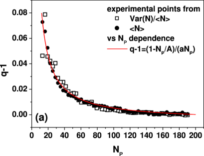
As shown in detail in OurPaper , this is precisely what is observed experimentally (cf., 1a). To recapitulate what was done there:
$(i)$ We know that if $U=$ const and $T=$ const then the multiplicity distribution $P(N)$ is Poissonian and we also know how fluctuations of $T$ change $P(N)$ from the Poissonian form to the NBD one.
$(ii)$ We want now to see how big are fluctuations of $T$ in our hadronizing systems formed in a collision process. It turns out that for $N=$ const we have either Eq. (4) or Eq. (3) depending on whether $T=$ const or $U=$ const. Assuming now validity of Eq. (1) not only in the above limiting cases but also in the general case when both the energy $U$ and the temperature $T$ fluctuate at the same time (fluctuations of the energy $U$ are given by Eq. 6) and corresponding fluctuations of the temperature $T$ are given by Eq. (7)).
$(iii)$ Knowing how big are fluctuations of $T$ we can deduce fluctuations of the multiplicity $N$.

Figure 1: (Color on line). $(a)$ Prediction of Eq. (8) versus experimental results obtained from $Var(N)/\langle N\rangle$ (squares) and from the $\langle N\rangle$ (circles) - see OurPaper for details. $(b)$ $Var(N)/\langle N\rangle$ for negatively charged particles produced in p+p, semicentral C+C, semicentral Si+Si, and Pb+Pb collisions as function of the fraction of nucleons participating in the collision, $N_{P}/A$, compared with our predictions (see OurPaper for details).

The analysis of different aspects of such fluctuations was performed in OurPaper and will not be repeated here. Instead we would like to bring ones attention to the following remarks. In the above formalism we have (cf. Eq. (B3) of OurPaper ) that $g_{T,N}(U)=[\beta/\Gamma(N)](\beta U)^{N-1}\exp(-\beta U)$ with fluctuations given by $Var(U)/\langle U\rangle^{2}=1/N$. In fact one can now invert distribution $g_{T,N}(U)$ (proceeding in analogous way as in Appendix B of OurPaper ) to obtain multiplicity distributions $g_{T,U}(N)$ and obtain distribution of temperature, $g_{U,N}(T)=\frac{\partial}{\partial\beta}\int_{0}^{U}g_{T,N}(U^{\prime})dU^{\prime}=[U/\Gamma(N)](\beta U)^{N-1}\exp(-\beta U)$ with fluctuations $Var(T)/\langle T\rangle^{2}\simeq Var(\beta)/\langle\beta\rangle^{2}=1/N$. The fluctuations of temperature obtained this way have gamma distribution. Because $C_{V}\propto N$ one obtains Eqs. (4) and (3). This illustrates that we can deduce fluctuations (i.e., the corresponding probability distributions) of any quantity out of ($T,U,N$) provided only that the other two are constant. The implication of this fact are still to be discussed.

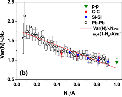
Let us return again to results of OurPaper . The Eq. (8) can be translated to direct dependence of $Var(N)/\langle N\rangle$ on the number of participants $N_{P}$, If $T_{eff}$ depends on $q$, i.e., if $T_{visc}\neq 0$ and there is some energy transfer from the hadronization region to the spectators, then the above dependence is connected with the dependence of $\langle N\rangle$ on $N_{P}$. The observed decreasing of $Var(N)/\langle N\rangle$ with $N_{P}$ implies then the nonlinear dependence of $\langle N\rangle$ on the number of participants $N_{P}$. It was also shown in OurPaper that $Var(N)/\langle N\rangle\propto 1-N_{P}/A$ (see Fig. 1b). In fact, also transverse momentum fluctuations defined by the measure $\Phi$ behave in the similar way: $\Phi\propto 1-N_{P}/A$. It means then that these fluctuations are reflecting not so much fluctuations of transverse momenta but rather fluctuations of the multiplicity.

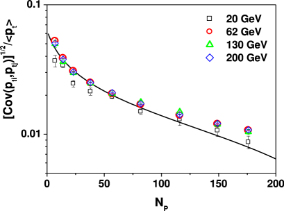
We would like to add here a new observation concerning behavior of correlations in transverse momenta measured in STAR . As shown in OurOld one can connect measure of fluctuations $\Phi$ with measured covariance in transverse momenta $Cov(p_{Ti},p_{Tj})$:

$$\Phi\left(\Phi\!+\!2\sqrt{Var\left(p_{t}\right)}\right)\! = \!\left(\langle N\rangle\!-\!1\!+Var(N)/\langle N\rangle\right)\cdot$$ (9)

$$\cdot Cov\left(p_{Ti},p_{Tj}\right).$$

Because we observe that $\Phi<<2\sqrt{Var\left(p_{T}\right)}$, one can write approximately that

$$\!\!\frac{Cov\left((p_{Ti},p_{Tj}\right)}{2\sqrt{Var(p_{T})}}\!\!\simeq\!\!\frac{\Phi}{\langle N\rangle\!-\!1\!+Var(N)/\langle N\rangle}\!=\!\frac{\Phi}{\langle N\rangle q}.$$ (10)

Using now relations derived in OurPaper one gets that

$$\frac{Cov\left((p_{Ti},p_{Tj}\right)}{2\sqrt{Var(p_{T})}}\simeq\frac{\Phi_{N_{P}=A}+b\left(1-\frac{N_{P}}{A}\right)}{n_{0}N_{P}+\frac{c+1}{a^{\prime}}\left(1-\frac{N_{P}}{A}\right)}.$$ (11)

Figure 2: (Color on line). Our results for correlations. Data are from STAR . The full line is our prediction as given by Eq. (11). See text for further details.

This is our prediction and it is shown in Fig. 2 for $\Phi_{N_{P}=A}=1.44$ MeV and for other parameters obtained from different comparisons with multiplicity fluctuations done in OurPaper , namely: $\langle p_{T}\rangle=400$ MeV, $b=4.8$ MeV, $n_{0}=0.642$, $c=4.1$, $a^{\prime}=1$ and $Var\left(p_{T}\right)/\langle p_{T}\rangle=0.43$. We stress here this fact because keeping the relevant independent parameters (altogether $4$ of them) as free, unconstrained by the multiplicity fluctuations data, would result in a simple formula which could fit data more exactly,

$$\!\!\frac{\sqrt{Cov\left(p_{Ti},p_{Tj}\right)}}{\langle p_{T}\rangle}\!\! = \!\!\sqrt{\frac{c_{1}+c_{2}\left(1\!-\!\frac{N_{P}}{A}\right)}{c_{3}N_{P}+c_{4}\left(1\!-\!\frac{N_{P}}{A}\right)}}.$$ (12)

To close let us stress again that our approach, which uses the $q$-statistics, allows to demonstrate the deep connection between fluctuations and correlations observed in transverse momenta and those observed in multiplicity distributions. It means that they all convey essentially the same information on the hadronizing system produced in high energy heavy ion collisions.

GW thanks the Organizers of the ISMD2009 for their warm hospitality during the conference.

References

- (1) Topical Issue on Statistical Power Law Tails in High-Energy Phenomena, Ed. Biró T S (2009) Eur. Phys. J. A 40(3).
- (2) Wilk G, and Włodarczyk Z (2009) Eur. Phys. J. A 40: 299 - 312.
- (3) Wilk G, Włodarczyk Z (2009) Phys. Rev C 79: 054903(10pp)
- (4) Lindhard J, ’Complementarity’ between energy and temperature, in The Lesson of Quantum Theory, Eds. de Boer J, Dal E, Ulfbeck O (1986) (North-Holland, Amsterdam).
- (5) Uffink J, and van Lith J (1999) Foundations of Phys. 29: 655 and Thermodynamic uncertainity relations, cond-mat/9806102.
- (6) Campisi M (2007) Phys. Lett. A 366: 335.
- (7) Adams J et al. (STAR Collab.) (2005) Phys. Rev. C 72: 044902 (6pp).
- (8) Utyuzh O V, Wilk G, Włodarczyk Z (2001) Phys. Rev. C 64: 027901 (4pp).