Clustering with shallow trees
Abstract
We propose a new method for hierarchical clustering based on the optimisation of a cost function over trees of limited depth, and we derive a message–passing method that allows to solve it efficiently. The method and algorithm can be interpreted as a natural interpolation between two well-known approaches, namely single linkage and the recently presented Affinity Propagation. We analyze with this general scheme three biological/medical structured datasets (human population based on genetic information, proteins based on sequences and verbal autopsies) and show that the interpolation technique provides new insight.
I Introduction
A standard approach to data clustering, that we will also follow here, involves defining a distance measure between objects, called dissimilarity. In this context, generally speaking data clustering deals with the problem of classifying objects so that objects within the same class or cluster are more similar than objects belonging to different classes. The choice of both the measure of similarity and the clustering algorithms are crucial in the sense that they define an underlying model for the cluster structure. In this work we discuss two somewhat opposite clustering strategies, and show how they nicely fit as limit cases of a more general scheme that we propose.
Two well-known general approaches that are extensively employed are partitioning methods and hierarchical clustering methods Flynn . Partitioning methods are based on the choice of a given number of centroids – i.e. reference elements – to which the other elements have to be compared. In this sense the problem reduces to finding a set of centroids that minimises the cumulative distance to points on the dataset. Two of the most used partitioning algorithms are -means (KM) and Affinity Propagation (AP)Leone ; Frey2007 . Behind these methods, there is the assumption of spherical distribution of data: clusters are forced to be loosely of spherical shape, with respect to the dissimilarity metric. These techniques give good results normally only when the structure underlying the data fits this hypothesis. Nevertheless, with Soft Affinity Propagation Leone the hard spherical constraint is relaxed, allowing for cluster structures including deviation from the regular shape. This method however recovers partially information on hierarchical organisation. On the other hand, Hierarchical Clustering methods such as single linkage (SL) Michael , starts by defining a cluster for each element of the system and then proceeds by repeatedly merging the two closest clusters into one. This procedure provides a hierarchic sequence of clusters.
Recently an algorithm to efficiently approximate optimum spanning trees with a maximum depth was presented in BaBoBrChRaZe2008 . We show here how this algorithm may be used to cluster data, in a method that can be understood as a generalisation of both (or rather an interpolation between) the AP and SL algorithms. Indeed in the and limits - where is the number of object to cluster - one recovers respectively AP and SL methods. As a proof of concept, we apply the new approach to a collection of biological and medical clustering problems on which intermediate values of provide new interesting results. In the next section, we define an objective function for clustering based on the cost of certain trees over the similarity matrix, and we devise a message-passing strategy to optimise the objective function. The following section is devoted to recovering two known algorithms, AP and SL, which are shown to be special cases for appropriately selected values of the external parameters . Finally, in the last section we use the algorithm on three biological/medical data clustering problems for which external information can be used to validate the algorithmic performance. First, we cluster human individuals from several geographical origins using their genetic differences, then we tackle the problem of clustering homologous proteins based only on their amino acid sequences. Finally we consider a clustering problem arising in the analysis causes-of-death in regions where vital registration systems are not available.
II A Common Framework
Let’s start with some definitions. Given datapoints, we introduce the similarity matrix between pairs , where . This interaction could be represented as a fully connected weighted graph where is the weight associated to each edge. This matrix contitutes the only data input for the clustering methods discussed in this manuscript. We refer in the following to the neighbourhood of node with the symbol , denoting the ensemble of all nearest neighbours of . By adding to the graph one artificial node , called root, whose similarity to all other nodes is a constant parameter , we obtain a new graph where is a matrix with one added row and column of constant value to the matrix (see Figure 1).

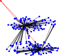
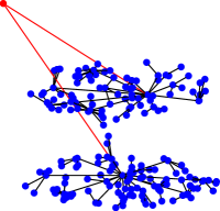
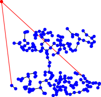
We will employ the following general scheme for clustering based on trees. Given any tree that spans all the nodes in the graph , consider the (possibly disconnected) subgraph resulting of removing the root and all its links. We will define the output of the clustering scheme as the family of vertex sets of the connected components of this subgraph. That is, each cluster will be formed by a connected component of the pruned . In the following, we will concentrate on how to produce trees associated to .
The algorithm described in BaBoBrChRaZe2008 was devised to find a tree of minimum weight with a depth bounded by from a selected root to a set of terminal nodes. In the clustering framework, all nodes are terminals and must be reached by the tree. As a tree has exactly links, for values of greater or equal than the problem becomes the familiar (unconstrained) minimum spanning tree problem. In the rest of this section we will describe the -MST message passing algorithm of BaBoBrChRaZe2008 for Steiner trees in the simplified context of (bounded depth) spanning trees.
To each node of the graph we associate two variables , and where could be interpreted as a pointer from to one of the neighbouring nodes . Meanwhile is thought as a discrete distance between the node and the root along the tree. Necessarily only the root has zero distance , while for all other nodes . In order to ensure global connectivity of the -MST, these two variables must satisfy the following condition: . This means that if node is the parent of node , then the depth of node must exceed the depth of the node by precisely one. This condition avoids the presence of loops and forces the graph to be connected, assigning non-null weight only to configurations corresponding to trees. The energy function thus reads
| (1) |
where is defined as
| (2) |
In this way only configurations corresponding to a tree are taken into account with the usual Boltzmann weight factor where the external parameter fixes the value of energy level. Thus the partition function is
| (3) |
where we have introduce an indicator function . Each term is equivalent to while is the delta function. In terms of these quantities it is possible to derive the cavity equations, i.e. the following set of coupled equations for the cavity marginal probability of each site after removing one of the nearest neighbours :
| (4) | |||
| (5) |
These equations are solved iteratively and in graphs with no cycles they are guaranteed to converge to a fixed point that is the optimal solution. In terms of cavity probability we are able to compute marginal and joint probability distribution using the following relations
| (6) | |||
| (7) |
For general graphs convergence can be forced by introducing a ”reinforcement” perturbation term as in BaBoBrChRaZe2008 ; braunstein2006learning . This leads to a new set of perturbed coupled equations that show good convergence properties. The limit is taken by considering the change of variable and then the relations 4 and 5 reduce to
| (8) | |||
| (9) |
These equations are in the Max-Sum form and equalities hold up to some additive constant. In terms of these quantities marginals are given by and the optimum tree is the one obtained by . If we introduce the variables , and it is enough to compute all the messages for and respectively. Using equations 8 and 9 we obtain the following set of equations:
| (10) | |||
| (11) | |||
| (12) |
It has been demonstrated spanningtree that a fixed point of these equations with depth is an optimal spanning tree. In the following two subsections, we show how to recover the SL and AP algorithms. On one hand, by computing the (unbounded depth) spanning tree on the enlarged matrix and then considering the connected components of its restriction to the set of nodes removing , we recover the results obtained by SL. On the other hand we obtain AP by computing the spanning tree rooted at , defining the self-affinity parameter as the weight to reach this root node.
II.1 Single Linkage limit
Single Linkage is one of the oldest and simplest clustering methods, and there are many possible descriptions of it. One of them is the following: order all pairs according to distances, and erase as many of the pairs with largest distance so that the number of resulting connected components is exactly . Define clusters as the resulting connected components.
An alternative method consists in removing initially all useless pairs (i.e. pairs that would not change the set of components when removed in the above procedure). This reduces to the following algorithm: given the distance matrix , compute the minimum spanning tree on the complete graph with weights given by . From the spanning tree remove the links with largest weight. Clusters are given by the resulting connected components. In many cases there is no a priori desired number of clusters and an alternative way of choosing is to use a continuous parameter to erase all weights larger than .
The -MST problem for identifies the minimum spanning tree connecting all nodes (including the root ). This means each node will point to one other node if its weight satisfies the condition , otherwise it would be cheaper to connect it to the root (introducing one more cluster). We will make this description more precise. For simplicity, let’s assume no edge in has weight exactly equal to .
The Kruskal algorithm Kruskal is a classical algorithm to compute a minimum spanning tree. It works by iteratively creating a forest as follows: start with a subgraph all nodes and no edges. The scan the list of edges ordered by increasing weight, and add the edge to the forest if it connects two different components (i.e. if it does not close a loop). At the end of the procedure, it is easy to prove that the forest has only one connected component that forms a minimum spanning tree. It is also easy to see that the edges added when applying the Kruskal algorithm to up to the point when the weight reaches are also admitted on the Kruskal algorithm for . After that point, the two procedures diverge because on the remaining added edges have weight larger than while on all remaining added edges have weight exactly . Summarizing, the MST on is a MST on on which all edges with weight greater than have been replaced by edges connecting with .
II.2 Affinity propagation limit
Affinity Propagation is a method that was recently proposed in
Frey2007 , based on the choice of a number of “exemplar”
data-points. Starting with a similarity matrix , choose a set of exemplar
datapoints and an assignment such that:
if and the sum of the distances between datapoints and the exemplars they map
to is minimised. It is essentially based on iteratively passing two
types of messages between elements, representing responsibility
and availability. The first, , measures how much
an element would prefer to choose the target as its
exemplar. The second tells the preference for to be
chosen as an exemplar by datapoint . This procedure
is an efficient implementation of the Max-Sum algorithm that improves
the naive exponential time complexity to . The
self-affinity parameter, namely , is chosen as the
dissimilarity of an exemplar with himself, and in fine
regulates the number of groups in the clustering procedure, by
allowing more or less points to link with “dissimilar”
exemplars.
Given a similarity matrix for nodes, we want to
identify the exemplars, that is, to find a valid configuration
such that so as to minimise the function
| (13) |
where the constraint reads
| (14) |
These equations take into account the only possible configurations, where node either is an exemplar, meaning , or it is not chosen as an exemplar by any other node . The energy function thus reads
| (15) |
The cavity equations are computed starting from this definition and after some algebra they reduce to the following update conditions for responsibility and availability Frey2007 :
| (16) | |||
| (17) |
In order to prove the equivalence between the two algorithms, i.e. -MST for and AP, we show in the following how the two employ an identical decomposition of the same energy function thus resulting necessarily to the same max sum equations. In the -MST equations, we are partitioning all nodes into three groups: the first one is only the root whose distance , the second one is composed of nodes pointing at the root and the last one is made up of nodes pointing to other nodes that have distance from the root. The following relations between and makes this condition explicit:
| (18) |
It is clear that the distance variable is redundant because the two kind of nodes are perfectly distinguished with just the variable . Going a step further we could remove the external root upon imposing the following condition for the pointers . This can be understood by thinking at AP procedure: since nodes at distance one from the root are the exemplars, they might point to themselves, as defined in AP, and all the non-exemplars are at distance so they might point to nodes at distance . Using this translation, from Equation 2 it follows that
| (19) |
meaning that the constraints are equivalent . Substituting (19) into equation (1) we obtain that
| (20) |
The identification of the self affinity parameter and the self similarity allows us to prove the equivalence between this formula and the AP energy given in equation (15) as desired.
A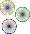 B
B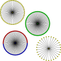 C
C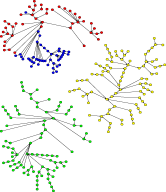 D
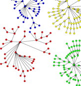
D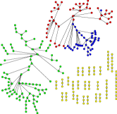
III Applications to biological data
In the following sections we shall apply the new technique to different clustering problems and give a preliminary comparison to the two extreme limits of the interpolation, namely (AP) and (SL).
Clustering is a widely used method of analysis in biology, most notably in the recents fields of transcriptomics Eisen1998 , proteomics and genomicsBarla2008 , where huge quantities of noisy data are generated routinely. A clustering approach presents many advantages for this type for data: it can use all pre-existing knowledge available to choose group numbers and to assign elements to groups, it has good properties of noise robustnessDougherty2002 , and it is computationally more tractable than other statistical techniques. In this section apply our algorithm to structured biological data, in order to show that by interpolating between two well-known clustering methods (SL and AP) it is possible to obtain new insight.
III.1 Multilocus genotype clustering
In this application we used the algorithm to classify individuals according to their original population using only information from their sequence SNPs as a distance measureaaa . A single-nucleotide polymorphism (SNP) is a DNA sequence variation occurring when a single nucleotide (A, T, C, or G) in the genome (or other shared sequence) differs between members of a species (or between paired chromosomes in a diploid individual). The dataset we used is from the HapMap Project, an international project launched in 2002 with the aim of providing a public resource to accelerate medical genetic research Hapmap . It consists of SNPs data from 269 individuals from four geographically diverse origins: 90 Utah residents from North and West Europe (CEU), 90 Yoruba of Ibadan, Nigeria (YRI), 45 Han Chinese of Beijing (CHB) and 44 Tokyo Japanese (JPT). CEU and YRI samples are articulated in thirty families of three people each, while CHB and JPT have no such structure. For each individual about 4 millions SNPs are given, allocated on different chromosomes. In the original dataset some SNPs were defined only in subpopulations, thus we extracted those which were well-defined for every sample in all populations and after this selection the number of SNPs for each individual dropped to million. We defined the distance between samples by the number of different alleles on the same locus among individuals normalised by the total number of counts. The matrix of distance was defined as follows:
| (21) |
where is the number of valid SNPs loci and is the distance between the -th genetic loci of individuals and :
| (22) |
The resulting distance matrix was given as input to -MST algorithm.
In figure 3 we show the clusters found by the algorithm
using a maximum depth . Each individual is represented by a
number and coloured according to the population he belongs to: green
for YRI, yellow for CEU, blue for JPT and red for CHB. One can see
that the algorithm recognises the populations grouping the individuals
in four clusters. There is only one misclassified case, a JPT
individual placed in the CHB cluster.
Moreover, noticing that yellow
and green clusters have a more regular internal structure than the
other two, it is possible to consider them separately. Therefore, if
one applies the -MST algorithm to this restricted subset of data,
all families consisting of three people can be immediately recovered,
and the tree subdivides in 60 families of 3 elements, without any
error (details not reported).
This dataset is particularly hard to classify, due to
the complexity of the distances distribution. In fact the presence of
families creates a sub-clustered structure inside the groups
of YRI and CEU individuals. Secondly CHB and JPT people,
even if they belong to different populations, share in general smaller
distances with respect to those subsisting among different families
inside one of the other two clusters.
The -MST algorithm overcomes this subtleties with the possibility
of developing a complex structure and allows the correct detection of
the four populations while other algorithms, such as AP, cannot adapt
to this variability of the typical distance scale between groups in the dataset.
Indeed, the hard constraint in AP relies strongly on cluster-shape
regularity and forces clusters to appear as star of radius one: there
is only one central node, and all other nodes are directly connected
to it. Elongated or irregular multi-dimensional data might have more
than one simple cluster centre. In this case AP may force division of
single clusters into separate ones or may group together different
clusters, according to the input self-similarities. Moreover, since
all data points in a cluster must point to the same exemplar, all
information about the internal structure, such as families grouping,
is lost. Thus, after running AP, CHB and JPT are grouped in a unique
cluster, and both CHB and JPT have the same exemplar, as shown on
figure 2A. Going a step further and forcing the algorithm
to divide Chinese from Japanese we start to split the YRI population
(Fig. 2B).
Hierarchical Clustering also fails on
this dataset, recognising the same three clusters found by
Affinity Propagation at the 3-clusters level (Fig. 2C) and
splitting yellow population in families before dividing blue from red
(see figure 2D). This makes sense relative to the typical
dissimilarities between individuals, but prevents grasping the
entire population structure.
After considering all four populations together, we applied the -MST algorithm only to the subset consisting of CHB and JPT individuals, because these data appeared the hardest to cluster correctly. The result is that the -MST algorithm, with depth succeeds in correctly detecting the two clusters without any miss-classification as shown in the left part of figure 4. Limiting the analysis to this selected dataset, Affinity Propagation identifies two different clusters, and is unable to divide CHB from JPT, still committing three mis-classifications, as viewed in right panel of the figure 4.
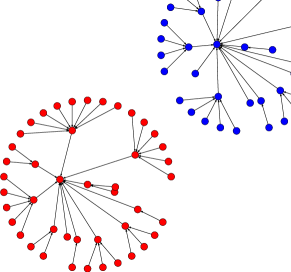
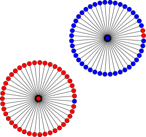
The cluster structure found is controlled both by the maximum depth and by , the two input parameters. In fact, in the extreme case all samples in the dataset would be forced to point to the root, representing a single cluster. The next step is and corresponds to Affinity Propagation. This allows to identify more than trivial clusters, as in the previous case, but, as we said, still imposes a strong constraint, which, in general, may be not representative of the effective data distribution. Increasing one can detect more structured clusters, where different elements in the same group do not necessary share a strong similarity with the same reference exemplar, as it has to be with Affinity Propagation or -means. On the other hand, the possibility to detect an articulated shape gives some information about the presence of eventual internal sub-structures notable to be analysed separately, as in our case the partition of two groups into families.
The parameter also affects the result of the clustering, in particular on the number of groups found. Assigning a large value to this parameter amounts to pay a high cost for every node connected to the root, and so to reduce the number of clusters; on the other side decreasing will create more clusters. In this first application we used a value of comparable with the typical distance between elements, allowing us to detect the four clusters. In this regime, one can expect a competition between the tendency of the elements to connect to other nodes or to form new clusters with links to the root, allowing the emergence of the underlying structure in the data.
III.2 Clustering of proteins datasets
An important computational problem is grouping proteins into families according to their sequence only. Biological evolution lets proteins fall into so-called families of similar proteins - in term of molecular function - thus imposing a natural classification. Similar proteins often share the same three-dimensional folding structure, active sites and binding domains, and therefore have very close functions. They often - but not necessarily - have a common ancestor, in evolutive terms. To predict the biological properties of a protein based on the sequence information alone, one either needs to be able to predict precisely its folded structure from its sequence properties, or to assign it to a group of proteins sharing a known common function. This second possibility stems almost exclusively from properties conserved in through the evolutionary time, and is computationally much more tractable than the first one. We want here to underline how our clustering method could be useful to handle this task, in a similar way as the one we used in the first application, by introducing a notion of distance between proteins based only on their sequences. The advantage of our algorithm is its global approach: we do not take into account only distances between a couple of proteins at a time, but we solve the clustering problem of finding all families in a set of proteins in a global sense. This allows the algorithm to detect cases where related proteins have low sequence identity.
To define similarities between proteins, we use the BLAST E-value as a
distance measure to assess whether a given alignment between two
different protein sequences constitutes evidence for homology. This
classical score is computed by comparing how strong an alignment is
with respect to what is expected by chance alone. This measure
accounts for the length of the proteins, as long proteins have more
chance to randomly share some subsequence. In essence, if the E-value
is 0 the match is perfect while the more E-value is high the more the
average similarity of the two sequences is low and can be considered
as being of no evolutionary relevance. We perform the calculation in
a all-by-all approach using the BLAST program, a sequence comparison
algorithm introduced by Altshul et al. Altshul .
Using this
notion of distance between proteins we are able to define a matrix of
similarity , in which each entry is associated to the
E-value between protein and . The -MST algorithm is then
able to find the directed tree between all the sets of nodes
minimising the same cost function as previously. The clusters we found
are compared to those computed by other clustering methods in the
literature, and to the “real” families of function that have been
identified experimentally.
As in the work by Paccanaro , we use the Astral 95 compendium of SCOP database SCOP where no two proteins share more than 95% of similarity, so as not to overload the clustering procedure with huge numbers of very similar proteins that could easily be attributed to a cluster by direct comparison if necessary. As this dataset is hierarchically organised, we choose to work at the level of superfamilies, in the sense that we want identify, on the basis of sequence content, which proteins belong to the same superfamily. Proteins belonging to the same superfamily are evolutionary related and share functional properties. Before going into the detail of the results we want to underline the fact that we do not modify our algorithm to adapt to this dataset structure, and without any prior assumption on the data, we are able to extract interesting information on the relative size and number of clusters selected (Fig.6). Notably we do not use a training set to optimise a model of the underlying cluster structure, but focus only on raw sequences and alignments.
One issue that was recently put forward is the alignment variability KarenM depending on the algorithms employed. Indeed some of our results could be biased by errors or dependence of the dissimilarity matrix upon the particular details of the alignments that are used to compute distances, but in the framework of a clustering procedure these small-scale differences should stay unseen due to the large scale of the dataset. On the other hand, the great advantage of working only with sequences is the opportunity to use our method on datasets where no structure is known a priori, such as fast developing metagenomics datasets Venter:2004 .
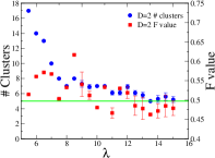
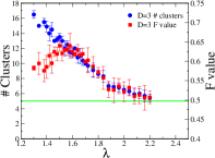
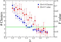
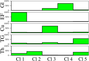
We choose as a training set different superfamilies belonging to the ASTRAL 95 compendium for a total number of 661 proteins: a) Globin-like, b) EF-hand, c) Cupredoxin, d) Trans-Glycosidases and e) Thioredoxin-like. Our algorithm is able to identify a good approximation on the real number of clusters. Here we choose the parameter well above the typical weight between different nodes, so as to minimise the number of groups found. As a function of this weight you can see the number of clusters found by the -MST algorithm reported in figure 5, for the depths . In these three plots we see the real value of the number of clusters is reached for different values of the weight respectively. The performance of the algorithm can be analysed in terms of precision and recall. These quantities are combined in the -value Paccanaro defined as
| (23) |
where is the number of nodes in cluster according to the classification we find with the -MST algorithm, is the number of nodes in the cluster according to the real cluster classification and is the number of predicted proteins in the cluster and at the same time in the cluster . In both cases the algorithm performs better results for lower value of . This could be related to the definition of the value because starting to reduce the number of expected clusters may be misleading in the accuracy of the predicted data clustering.
Since distances between datapoints have been normalised to be real numbers between to , when we expect to find the number of connected components of the given graph . While lowering this value, we start to find some configurations which minimise the weight respect to the single cluster solution. The role played by the external parameter could be seen as the one played by a chemical potential tuning from outside the average number of clusters.
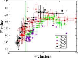
We compare our results to the ones in Paccanaro for different algorithms and it is clear that intermediate values of gives best results on the number of clusters detected and on the -value reached without any a priori treatment of data. It is also clear that -MST algorith mwith gives better results than AP (case ) as can be seen in Fig. 7.
We believe that the reason is that clusters do not have an intrinsic spherical regularity. This may be due to the fact that two proteins having a high number of differences between their sequences at irrelevant sites can be in the same family. Such phenomena can create clusters with complex topologies in the sequence space, hard to recover with methods based on a spherical shape hypothesis. We compute the -value also in the single linkage limit () and its value is almost in all the range of clusters detected. This shows that the quality of the predicted clusters improves reaching the highest value when and then decreases when the maximum depth increases.
III.3 Clustering of verbal autopsy data
The verbal autopsy is an important survey-based approach to measuring cause-specific mortality rates in populations for which there is no vital registration system MurrayLFPY2007 ; KingL2008 . We applied our clustering method to the results of 2039 questionnaires in a benchmark verbal autopsy dataset, where gold-standard cause-of-death diagnosis is known for each individual. Each entry in the dataset is composed of responses 47 yes/no/don’t know questions.
To reduce the effect of incomplete information, we restricted our analysis to the responses for which at least 91% of questions answered yes or no (in other words, at most 9% of the responses were “don’t know”). This leaves 743 responses to cluster (see MurrayLFPY2007 for a detailed descriptive analysis of the response patterns in this dataset.)
The goal of clustering verbal autopsy responses is to infer the common causes of death on the basis of the answers. This could be used in the framework of “active learning”, for example, to identify which verbal autopsies require further investigation by medical professionals.
As in the previous applications, we define a distance matrix on the verbal autopsy data and apply -MST with different depths . The questionnaires are turned into vectors by associating to the answers yes/no/don’t know the values 0/1/0.5 respectively. The similarity matrix is then computed as the root mean square difference between vectors, , where refers to the symptom in the i-th questionnaire.
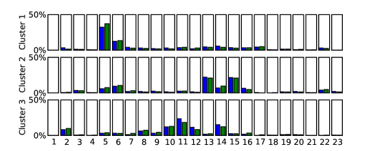
We first run -MST (AP) and -MST on the dataset and find how the number of clusters depend on . We identify a stable region which corresponds to 3 main clusters for both . As shown in figure 8, to each cluster we can associate a different causes of death. Cluster 1 contains nearly all of the Ischemic Heart Disease deaths (cause 5) and about half of the Diabetes Mellitus deaths (cause 6). Cluster 2 contains most of the Lung Cancer deaths (cause 13) and Chronic Obstructive Pulmonary Disease deaths (cause 15). Cluster 2 also contains most of the additional IHD and DM deaths (30% of all deaths in the dataset are due to IHD and DM). Cluster 3 contains most of the Liver Cancer deaths (cause 11) as well as most of the Tuberculosis deaths (cause 2) and some of the other prevalent causes. For we find no distinguishable hierarchical structure in the 3 clusters, while for higher value we find a second-level structure. In particular for we obtain 57-60 subfamilies for value of in the region of . Although the first-level analysis (Fig.8B) underlines the similarity of -MST algorithm with AP, increasing the depth leads to a finer sub-clusters decomposition progress .
III.4 Conclusion
We introduced a new clustering algorithm which naturally interpolates between partitioning methods and hierarchical clustering. The algorithm is based on the cavity method and finds a bounded depth spanning tree on a graph where is the set of vertices identified with the data points plus one additional root node and is the set of edges with weights given by the dissimilarity matrix and by a unique distance from the root node. The limits and reduce to the well known AP and SL algorithms. The choice of determines the number of clusters. Here we have adopted the same criterion as in ref. Frey2007 : the first non trivial clustering occurs when the cluster number is constant for a stable region of values.
Preliminary applications on three different biological datasets have shown that it is indeed possible to exploit the deviation from the purely spherical limit to gain some insight into the data structures. Our method has properties which are of generic relevance for large scale datasets, namely scalability, simplicity and parallelizability. Work is in progress to systematically apply this technique to real world data.
Acknowledgements.
The work was supported by a Microsoft External Research Initiative grant. SB acknowledges MIUR grant 2007JHLPEZ.References
- [1] A. K. Jain, M. N. Murty, and P. J. Flynn. Data clustering: a review. ACM Comput. Surv., 31(3):264–323, 1999.
- [2] M. Leone, S. Sumedha, and M. Weigt. Clustering by soft-constraint affinity propagation: applications to gene-expression data. Bioinformatics, 23:2708, 2007.
- [3] Brendan J. J. Frey and Delbert Dueck. Clustering by passing messages between data points. Science, 315:972–976, February 2007.
- [4] Michael B. Eisen, Paul T. Spellman, Patrick O. Brown, and David Botstein. Cluster analysis and display of genome-wide expression patterns. Proceedings of the National Academy of Sciences of the United States of America, 95(25):14863–14868, 1998.
- [5] M. Bayati, C. Borgs, A. Braunstein, J. Chayes, A. Ramezanpour, and R. Zecchina. Statistical Mechanics of Steiner Trees. Physical Review Letters, 101(3):37208, 2008.
- [6] A. Braunstein and R. Zecchina. Learning by message passing in networks of discrete synapses. Physical Review Letters, 96(3):30201, 2006.
- [7] Mohsen Bayati, Alfredo Braunstein, and Riccardo Zecchina. A rigorous analysis of the cavity equations for the minimum spanning tree. Journal of Mathematical Physics, 49(12):125206, 2008.
- [8] Joseph B. Kruskal. On the shortest spanning subtree of a graph and the traveling salesman problem. Proceedings of the American Mathematical Society, 7(1):48–50, February 1956.
- [9] M. B. Eisen, P. T. Spellman, P. O. Brown, and D. Botstein. Cluster analysis and display of genome-wide expression patterns. Proc Natl Acad Sci U S A, 95(25):14863–14868, Dec 1998.
- [10] Annalisa Barla, Giuseppe Jurman, Samantha Riccadonna, Stefano Merler, Marco Chierici, and Cesare Furlanello. Machine learning methods for predictive proteomics. Brief Bioinform, 9(2):119–128, Mar 2008.
- [11] Edward R Dougherty, Junior Barrera, Marcel Brun, Seungchan Kim, Roberto M Cesar, Yidong Chen, Michael Bittner, and Jeffrey M Trent. Inference from clustering with application to gene-expression microarrays. J Comput Biol, 9(1):105–126, 2002.
- [12] Xiaoyi Gao and Joshua Starmer. Human population structure detection via multilocus genotype clustering. BMC Genetics, 8(1):34, 2007.
- [13] The International HapMap Consortium. A second generation human haplotype map of over 3.1 million snps. Nature, 449:851, 2007.
- [14] S. F. Altschul, W. Gish, W. Miller, E. W. Myers, and D. J. Lipman. Basic local alignment search tool. J. Mol. Biol., 215:403, 1990.
- [15] A. Paccanaro, J. A. Casbon, and M.A.S. Saqi. Spectral clustering of protein sequnces. Nucleid Acid Research, 34:1571, 2006.
- [16] A.G. Murzin, S.E. Brenner, T. Hubbard, and C. Chothia. Scop: A structural classification of proteins database for the investigation of sequnces and structures. J. Mol. Biol., 247:536, 1995.
- [17] Karen M. Wong, Marc A. Suchard, and John P. Huelsenbeck. Alignment Uncertainty and Genomic Analysis. Science, 319(5862):473–476, 2008.
- [18] JC Venter, K Remington, JF Heidelberg, AL Halpern, and D Rusch. Environmental genome shotgun sequencing of the sargasso sea. Science, 304:66–74, 2004.
- [19] Christopher J. L Murray, Alan D Lopez, Dennis M Feehan, Shanon T Peter, and Gonghuan Yang. Validation of the symptom pattern method for analyzing verbal autopsy data. PLoS Med, 4(11):e327, 11 2007.
- [20] Gary King and Ying Lu. Verbal autopsy methods with multiple causes of death. Statistical Science, 23(1):78–91, 2008.
- [21] S. Bradde, A. Braunstein, A. Flaxman, and R. Zecchina. in progress.