Constraining the time variation of the coupling constants from cosmic microwave background: effect of ΛQCDsubscriptΛQCD\Lambda_{\mathrm{QCD}}

Masahiro Nakashima 1,2    Kazuhide Ichikawa 3    Ryo Nagata 2    Jun’ichi Yokoyama 2,4 1 Department of Physics, Graduate School of Science,
The University of Tokyo, Tokyo 113-0033, Japan
2 Research Center for the Early Universe (RESCEU),
Graduate School of Science, The University of Tokyo, Tokyo 113-0033, Japan
3 Department of Micro Engineering, Kyoto University, Kyoto 606-8501, Japan
4 Institute for the Physics and Mathematics of the Universe(IPMU),
The University of Tokyo, Kashiwa, Chiba, 277-8568, Japan
Abstract

We investigate constraints on the time variation of the fine structure constant between the recombination epoch and the present epoch, Δα/α(αrecαnow)/αnowΔ𝛼𝛼subscript𝛼recsubscript𝛼nowsubscript𝛼now\Delta\alpha/\alpha\equiv(\alpha_{\mathrm{rec}}-\alpha_{\mathrm{now}})/\alpha_{\mathrm{now}}, from cosmic microwave background (CMB) taking into account simultaneous variation of other physical constants, namely the electron mass mesubscript𝑚𝑒m_{e} and the proton mass mpsubscript𝑚𝑝m_{p}. In other words, we consider the variation of Yukawa coupling and the QCD scale ΛQCDsubscriptΛQCD\Lambda_{\mathrm{QCD}} in addition to the electromagnetic coupling. We clarify which parameters can be determined from CMB temperature anisotropy in terms of singular value decomposition. Assuming a relation among variations of coupling constants governed by a single scalar field (the dilaton), the 95 % confidence level (C.L.) constraint on Δα/αΔ𝛼𝛼\Delta\alpha/\alpha is found to be 8.28×10³<Δα/α<1.81×1038.28superscript103Δ𝛼𝛼1.81superscript103-8.28\times 10^{-3}<\Delta\alpha/\alpha<1.81\times 10^{-3}, which is tighter than the one obtained by considering only the change of α𝛼\alpha and mesubscript𝑚𝑒m_{e}. We also obtain the constraint on the time variation of the proton-to-electron mass ratio μmp/me𝜇subscript𝑚𝑝subscript𝑚𝑒\mu\equiv m_{p}/m_{e} to be 0.52<Δμ/μ<0.170.52Δ𝜇𝜇0.17-0.52<\Delta\mu/\mu<0.17 (95 % C.L.) under the same assumption. Finally, we also implement a forecast for constraints from the PLANCK survey.

RESCEU-25-09

I Introduction

Whether or not the physical constants are truly constant is not only a fundamental issue in physics but also an important probe of the theories of extra dimensions. Since the early studies of Dirac Dirac:1937ti ; Dirac:1938mt , many theoretical models that could accomodate the variation of physical constants have been proposed Bekenstein:1982eu ; Barrow:2001iw ; Barrow:2005qf ; Uzan:2002vq ; Chiba:2006xx . Unification theories such as superstring theories predict the existence of an additional scalar field ΦΦ\Phi called “dilaton” and the destabilization of this field Dine:1985he ; Brustein:1992nk might cause the variation of coupling constants. In more phenomenological contexts, dynamical scalar fields introduced to explain the recent discovery of the accerelated expansion may be non-minimally coupled to gauge fields in the Standard model, which may also lead to time varying coupling constants Avelino:2006gc ; Avelino:2008dc ; Fujii:2007zg ; Fujii:2008zj ; Dent:2008vd ; Avelino:2009fd . Thus, investigating the variation of the coupling constants can be an important probe of these theories.

Not only these theoretical sides but also the observational analysis of various systems have been playing an important role in the investigation of the time variation of physical constants. Among them, the claim for the deviation of the past value of the fine structure constant α𝛼\alpha from the present one by using the high-redshift quasar absorption system Webb:1998cq ; Webb:2000mn had the great impact on this topic. Further analysis for the quasar absorption spectra gives the support for this positive result of a cosmological variation of α𝛼\alpha Murphy:2004 ; Murphy:2006vs ; Murphy:2007qs ; Molaro:2007kp , though some authors takes objection to such variations Chand:2004ct ; Srianand:2004mq ; Molaro:2007kp .

Stimulated by these studies from both theoretical and observational sides, various constraints on the time variation of the fine structure constant α𝛼\alpha have been investigated from diverse observations. We briefly summarize those terrestrial and celestial limits on α𝛼\alpha as follows (see Uzan:2002vq ; Chiba:2001ui for a review). The atomic clocks constrain the current value of the temporal derivative of α𝛼\alpha as α˙/α=(3.3±3.0)×1016yr1˙𝛼𝛼plus-or-minus3.33.0superscript1016superscriptyr1\dot{\alpha}/\alpha=(-3.3\pm 3.0)\times 10^{-16}\ \mathrm{yr}^{-1}Blatt:2008su ; Fortier:2007jf ; Peik:2004qn ; Fischer:2004jt . The measurement of the frequency ratio of aluminium and mercury single-ion optical clocks provides α˙/α=(1.6±2.3)×1017yr1˙𝛼𝛼plus-or-minus1.62.3superscript1017superscriptyr1\dot{\alpha}/\alpha=(-1.6\pm 2.3)\times 10^{-17}\ \mathrm{yr}^{-1} Rosenband:2008 . From the analysis of Sm isotopes in the Oklo natural reactor in Gabon, we get two bounds on the variation of α𝛼\alpha as Δα/α=(0.8±1.0)×108Δ𝛼𝛼plus-or-minus0.81.0superscript108\Delta\alpha/\alpha=-(0.8\pm 1.0)\times 10^{-8} and Δα/α=(0.88±0.07)×107Δ𝛼𝛼plus-or-minus0.880.07superscript107\Delta\alpha/\alpha=(0.88\pm 0.07)\times 10^{-7} Fujii:2002hc , which measures the value at the redshift z0.1similar-to𝑧0.1z\sim 0.1 constraint. From the spectra of quasars, several limits have been obtained using various data sets: Δα/α=(0.57±0.11)×105(z0.24.2\Delta\alpha/\alpha=(-0.57\pm 0.11)\times 10^{-5}\ (z\sim 0.2-4.2) from the Keck/HIRES instrument Murphy:2004 , Δα/α=(0.64±0.36)×105(z0.42.3)Δ𝛼𝛼plus-or-minus0.640.36superscript105similar-to𝑧0.42.3\Delta\alpha/\alpha=(-0.64\pm 0.36)\times 10^{-5}\ (z\sim 0.4-2.3) from the Ultraviolet and Visual Echelle Spectrograph (UVES) instrument Murphy:2006vs ; Murphy:2007qs . Big bang nucleosynthesis (BBN) provides constraints at very high redshifts (z1091010similar-to𝑧superscript109superscript1010z\sim 10^{9}-10^{10}), for example, 5.0×10²<Δα/α<1.0×102(95%C.L.)-5.0\times 10^{-2}<\Delta\alpha/\alpha<1.0\times 10^{-2}\ (95\%\mathrm{C.L.}) Ichikawa:2002bt . Finally, Cosmic Microwave Background (CMB) measures α𝛼\alpha at z103similar-to𝑧superscript103z\sim 10^{3} and the limits from WMAP 1-year, 3-year and 5-year data read 0.06<Δα/α<0.010.06Δ𝛼𝛼0.01-0.06<\Delta\alpha/\alpha<0.01 Rocha:2003gc , 0.039<Δα/α<0.0100.039Δ𝛼𝛼0.010-0.039<\Delta\alpha/\alpha<0.010 Stefanescu:2007aa and 0.028<Δα/α<0.0260.028Δ𝛼𝛼0.026-0.028<\Delta\alpha/\alpha<0.026 Nakashima:2008cb respectively, all of which are at 95%C.L.formulae-sequencepercent95CL95\%\mathrm{C.L.} Recently, Menegoni et al. Menegoni:2009rg obtained more improved result 0.013<Δα/α<0.0150.013Δ𝛼𝛼0.015-0.013<\Delta\alpha/\alpha<0.015 at 95%C.L.formulae-sequencepercent95CL95\%\mathrm{C.L.} from WMAP 5-year date combined with ACBAR, QUAD and BICEP experiments data.

Along with α𝛼\alpha, several observational constraints have been obtained on another physical constant, the proton-to-electron mass ratio μmp/me𝜇subscript𝑚𝑝subscript𝑚𝑒\mu\equiv m_{p}/m_{e}. As in α𝛼\alpha, atomic clocks very tightly constrain the current value of its temporal derivative as μ˙/μ=(1.5±1.7)×1015yr1˙𝜇𝜇plus-or-minus1.51.7superscript1015superscriptyr1\dot{\mu}/\mu=(-1.5\pm 1.7)\times 10^{-15}\ \mathrm{yr}^{-1}Blatt:2008su . Reinhold et al. Reinhold:2006zn reports the non-vanishing variation of μ𝜇\mu as Δμ/μ=(2.4±0.6)×105Δ𝜇𝜇plus-or-minus2.40.6superscript105\Delta\mu/\mu=(2.4\pm 0.6)\times 10^{-5} from a weighted sum of accurate H2subscriptH2\mathrm{H}_{2} spectral lines in two quasar systems (corresponding redshifts are z=2.59𝑧2.59z=2.59 and z=3.02𝑧3.02z=3.02). Based on the quasar absorption spectra of NH3subscriptNH3\mathrm{NH}_{3}, the limit is Δμ/μ=(0.6±1.9)×106Δ𝜇𝜇plus-or-minus0.61.9superscript106\Delta\mu/\mu=(0.6\pm 1.9)\times 10^{-6} at z=0.6847𝑧0.6847z=0.6847 Flambaum:2007fa and further detailed measurement by the same method tighten the bound as Δμ/μ=(0.74±0.47)×106Δ𝜇𝜇plus-or-minus0.740.47superscript106\Delta\mu/\mu=(0.74\pm 0.47)\times 10^{-6} Murphy:2008yy .

In this paper, using WMAP 5-year data, we focus on the CMB constraint on α𝛼\alpha in the case that the multiple physical constants may vary with time simultaneously according to the expectation values of a single dilaton field ΦΦ\Phi. Although similar analyses has been done for BBN Ichikawa:2002bt ; Campbell:1994bf ; Langacker:2001td ; Dent:2001ga ; Muller:2004gu ; Dent:2008gx , quasar absorption system Calmet:2001nu ; Calmet:2002ja or the Oklo reactor Olive:2002tz , few attempts from CMB data have been made except for several preceding literatures Ichikawa:2006nm ; Landau:2008re ; Scoccola:2008jw , which treated simultaneous variations of only α𝛼\alpha and mesubscript𝑚𝑒m_{e}. In addition to α𝛼\alpha and mesubscript𝑚𝑒m_{e}, many theoretical models predict the time variation of the QCD scale ΛQCDsubscriptΛQCD\Lambda_{\mathrm{QCD}} (which results from the variation of the strong coupling constant), so it is important to include the ΛQCDsubscriptΛQCD\Lambda_{\mathrm{QCD}} effect in the analysis. We consider the effect of varying ΛQCDsubscriptΛQCD\Lambda_{\mathrm{QCD}} as the change in the proton mass mpsubscript𝑚𝑝m_{p} which is assumed to be proportional to ΛQCDsubscriptΛQCD\Lambda_{\mathrm{QCD}} 111When we consider the time variation of ΛQCDsubscriptΛQCD\Lambda_{\mathrm{QCD}}, the neutron mass also changes. In this paper, we neglect the difference between the proton mass and the neutron mass, and when we refer to the time variation of the proton mass mpsubscript𝑚𝑝m_{p}, we implicitly include the time variation of the neutron mass assuming that the neutron mass changes in exactly the same way as the proton mass. . Thus, we consider simultaneous variation of α𝛼\alpha, mesubscript𝑚𝑒m_{e} and mpsubscript𝑚𝑝m_{p}. Since how the variation of ΛQCDsubscriptΛQCD\Lambda_{\mathrm{QCD}} is related to that of α𝛼\alpha or mesubscript𝑚𝑒m_{e} depends on the details of the unification model Dine:2002ir , we here adopt a specific example of the relation among those physical constants following Ichikawa:2002bt or Campbell:1994bf , which is based on a low energy effective theory of string theory. The newly incorporated change of ΛQCDsubscriptΛQCD\Lambda_{\mathrm{QCD}} leads to a new and tighter constraint on the time variation of α𝛼\alpha. We also obtain a constraint on μ𝜇\mu induced by the time dependence of ΛQCDsubscriptΛ𝑄𝐶𝐷\Lambda_{QCD} and mesubscript𝑚𝑒m_{e}.

This paper is organized as follows. Section II provides how the variation of each physical constant affects the CMB power spectrum both qualitatively and quantitatively with particular attention to ΛQCDsubscriptΛQCD\Lambda_{\mathrm{QCD}}. Section III briefly describes the model we adopt based on string theory which governs the time evolution of the three physical constants we consider, namely, the variation of the fine structure constant, the electron mass and the proton mass. In section IV, we provide the limits of those variations. Section V is devoted to conclusion. The details of the calculations of the degeneracy and parameter dependence are given in the appendix A. In appendix B, we present a forecast for constraints from the PLANCK experiment.

II The effect of variations of physical constants on the CMB

As is well known, a primary CMB photon is a relic signal from the last scattering surfuce about thirteen billion years ago, which means that the most important process for CMB photon is the recombination. It has been known that changing the value of the fine structure constant α𝛼\alpha and the electron mass mesubscript𝑚𝑒m_{e} affects the CMB power spectrum mainly through the change of the epoch of recombination Hannestad:1998xp ; Kaplinghat:1998ry ; Kujat:1999rk ; Yoo:2002vw . The larger value of α𝛼\alpha or mesubscript𝑚𝑒m_{e} at the recombination epoch causes the higher redshift of the last scattering surface because the hydrogen binding energy scales as α2mesuperscript𝛼2subscript𝑚𝑒\alpha^{2}m_{e}. This results in three characteristic signatures in the angular power spectrum of the temperature anisotropy, namely, shift of the peaks to higher multipoles, increase of the height of the peaks due to the enhanced early integrated Sachs Wolfe effect, and decrease of the small-scale diffusion damping effect. To be more precise, however, the process of the recombination depend on α𝛼\alpha and mesubscript𝑚𝑒m_{e} in a subtly different manner as will be explicitly shown in eqs.(6)-(9) in the argument of the four CMB-characteristic variables below.

The time variation of the proton mass mpsubscript𝑚𝑝m_{p} affects the CMB power spectrum mainly through the baryon density ρBsubscript𝜌𝐵\rho_{B}. In the standard cosmology with no variation of physical constants, the baryon density scales as ρB,rec=ρB,0(a0/arec)3subscript𝜌𝐵recsubscript𝜌𝐵0superscriptsubscript𝑎0subscript𝑎rec3\rho_{B,\mathrm{rec}}=\rho_{B,\mathrm{0}}(a_{\mathrm{0}}/a_{\mathrm{rec}})^{3}, where a𝑎a is the scale factor and the subscripts “rec” and “0” denote values at the epoch of recombination and the present epoch, respectively. When we allow the time variation of mpsubscript𝑚𝑝m_{p}, there is an additional change as

ρB,rec=ρB,0(a0arec)3mp,recmp,0ρB,0(a0arec)3(1+Δmpmp),subscript𝜌𝐵recsubscript𝜌𝐵0superscriptsubscript𝑎0subscript𝑎rec3subscript𝑚𝑝recsubscript𝑚𝑝0subscript𝜌𝐵0superscriptsubscript𝑎0subscript𝑎rec31Δsubscript𝑚𝑝subscript𝑚𝑝\rho_{B,\mathrm{rec}}=\rho_{B,\mathrm{0}}\left(\frac{a_{\mathrm{0}}}{a_{\mathrm{rec}}}\right)^{3}\frac{m_{p,\mathrm{rec}}}{m_{p,\mathrm{0}}}\equiv\rho_{B,\mathrm{0}}\left(\frac{a_{\mathrm{0}}}{a_{\mathrm{rec}}}\right)^{3}\left(1+\frac{\Delta m_{p}}{m_{p}}\right), (1)

where we define Δmpmp,recmp,0Δsubscript𝑚𝑝subscript𝑚𝑝recsubscript𝑚𝑝0\Delta m_{p}\equiv m_{p,\mathrm{rec}}-m_{p,\mathrm{0}}. Therefore, the effect of changing mp,recsubscript𝑚𝑝recm_{p,\mathrm{rec}} is very similar to changing ρB,0subscript𝜌𝐵0\rho_{B,\mathrm{0}}. One may even consider that mp,recsubscript𝑚𝑝recm_{p,\mathrm{rec}} and ρB,0subscript𝜌𝐵0\rho_{B,\mathrm{0}} are totally degenerate. However, there appears a subtle difference as regards the baryon number density nBsubscript𝑛𝐵n_{B} which affects the recombination process. This is because, contrary to the case of ρBsubscript𝜌𝐵\rho_{B}, the scaling nB,rec=nB,0(a0/arec)3subscript𝑛𝐵recsubscript𝑛𝐵0superscriptsubscript𝑎0subscript𝑎rec3n_{B,\mathrm{rec}}=n_{B,\mathrm{0}}(a_{\mathrm{0}}/a_{\mathrm{rec}})^{3} is not affected by the variation of mpsubscript𝑚𝑝m_{p} (note that nBρB/mpsubscript𝑛𝐵subscript𝜌𝐵subscript𝑚𝑝n_{B}\equiv\rho_{B}/m_{p}). Thus, suppose one increases ρB,0subscript𝜌𝐵0\rho_{B,\mathrm{0}} and decreases mp,recsubscript𝑚𝑝recm_{p,\mathrm{rec}} while preserving the value of ρB,recsubscript𝜌𝐵rec\rho_{B,\mathrm{rec}}, nB,recsubscript𝑛𝐵recn_{B,\mathrm{rec}} is increased. This is the reason why varying ρB,0subscript𝜌𝐵0\rho_{B,\mathrm{0}} (as is done in the usual parameter search) and varying mp,recsubscript𝑚𝑝recm_{p,\mathrm{rec}} are different and we can break the degeneracy between them in the parameter estimation although the degeneracy turns out to be rather strong.
Refer to caption
Refer to caption
Refer to caption
Refer to caption
Refer to caption
Refer to caption
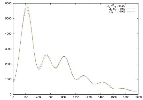
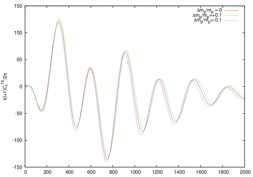
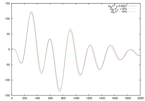
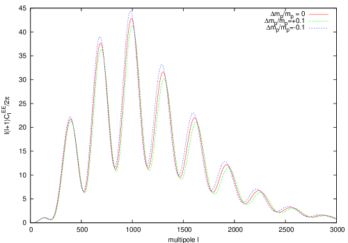
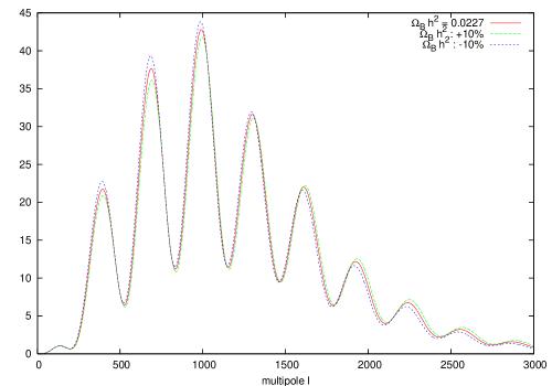
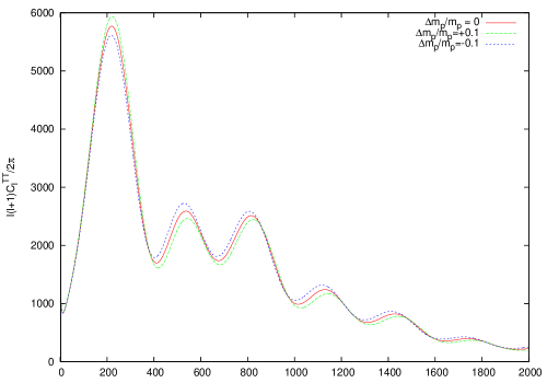
Figure 1: The top left panel is the CMB temperature anisotropy spectra for no change of mpsubscript𝑚𝑝m_{p} (solid red curve), an increase of mpsubscript𝑚𝑝m_{p} by 10%percent\% (dashed green curve), a decrease of mpsubscript𝑚𝑝m_{p} by 10%percent\% (dotted blue curve). The middle left and bottom left panels are the TE and EE spectra respectively for three different values of Δmp/mpΔsubscript𝑚𝑝subscript𝑚𝑝\Delta m_{p}/m_{p}. For comparison, the corresponding spectra for three different values of ΩBh2subscriptΩ𝐵superscript2\Omega_{B}h^{2} are shown in the right hand side panels.

With the careful attention to the difference between ρBsubscript𝜌𝐵\rho_{B} and ΔmpΔsubscript𝑚𝑝\Delta m_{p} noted in the last paragraph, we calculated the angular power spectra of the CMB temperature anisotropy, CTTsuperscriptsubscript𝐶𝑇𝑇C_{\ell}^{TT}, for several different values of ΔmpΔsubscript𝑚𝑝\Delta m_{p} using the modified CAMB code camb . The result is shown in FIG. 1, where we also draw the cross correlation of temperature and E-mode polarization, CTEsuperscriptsubscript𝐶𝑇𝐸C_{\ell}^{TE}, and the angular power spectrum of E-mode polarization, CEEsuperscriptsubscript𝐶𝐸𝐸C_{\ell}^{EE}, for completeness. Incorporating ΔmpΔsubscript𝑚𝑝\Delta m_{p} into the numerical calculation, we assume mpsubscript𝑚𝑝m_{p} to change instantaneously at a specific time (z=100𝑧100z=100). In other words, mp,recsubscript𝑚𝑝recm_{p,\mathrm{rec}} was constant before z=100𝑧100z=100 and after that the proton mass becomes the present value 222Here, only the mass difference ΔmpΔsubscript𝑚𝑝\Delta m_{p} matters and it is not important how the proton mass has changed between the recombination epoch and the present epoch, because characteristic signatures such as acoustic oscillation or Silk damping are imprinted before and during the recombination process, which is also true on the effects that ΔmpΔsubscript𝑚𝑝\Delta m_{p} induces.. This procedure is adopted throughout this paper. We consider a flat ΛΛ\LambdaCDM universe with a power-law adiabatic primordial fluctuation and take the fiducial standard cosmological parameter values as the WMAP 5-year marginalized mean values Dunkley:2008ie ; Komatsu:2008hk ;

(ΩBh2,ΩDMh2,h,τ,ns)=(0.0227,0.1099,0.72,0.087,0.963),subscriptΩ𝐵superscript2subscriptΩ𝐷𝑀superscript2𝜏subscript𝑛𝑠0.02270.10990.720.0870.963(\Omega_{B}h^{2},\Omega_{DM}h^{2},h,\tau,n_{s})=(0.0227,0.1099,0.72,0.087,0.963), (2)

where ΩBsubscriptΩ𝐵\Omega_{B} is the baryon energy density ρB,0subscript𝜌𝐵0\rho_{B,\mathrm{0}} normalized by the critical density ρcrit,0subscript𝜌crit0\rho_{\mathrm{crit,0}}, ΩDMsubscriptΩ𝐷𝑀\Omega_{DM} is the dark matter energy density ρDM,0subscript𝜌𝐷𝑀0\rho_{DM,\mathrm{0}} normalized by the critical density ρcrit,0subscript𝜌crit0\rho_{\mathrm{crit,0}}, hh is the current Hubble parameter, H0subscript𝐻0H_{0}, in units of 100 km sec-1 Mpc-1, τ𝜏\tau is the optical depth to reionization and nssubscript𝑛𝑠n_{s} is the spectral index of the primordial curvature perturbation. As expected from the above argument, the effect of ΔmpΔsubscript𝑚𝑝\Delta m_{p} is very similar to that of ΩBsubscriptΩ𝐵\Omega_{B}. Due to the larger value of ΔmpΔsubscript𝑚𝑝\Delta m_{p}, the height of the odd peaks increases compared with that of the even peaks, which is a very well-known result for ΩBsubscriptΩ𝐵\Omega_{B} Hu:1995en .

Now we discuss how the variations of the parameters change the shape of the CMB power spectrum quantitatively. We use four quantities which have been proposed to characterize the temperature spectrum well Hu:2000ti : the position of the first peak 1subscript1\ell_{1}, the height of the first peak relative to the large angular-scale amplitude evaluated at =1010\ell=10,

H1(ΔT1ΔT10)2,subscript𝐻1superscriptΔsubscript𝑇subscript1Δsubscript𝑇102H_{1}\equiv\left(\frac{\Delta T_{\ell_{1}}}{\Delta T_{10}}\right)^{2}, (3)

the ratio of the second peak 2subscript2\ell_{2} height to the first,

H2(ΔT2ΔT1)2,subscript𝐻2superscriptΔsubscript𝑇subscript2Δsubscript𝑇subscript12H_{2}\equiv\left(\frac{\Delta T_{\ell_{2}}}{\Delta T_{\ell_{1}}}\right)^{2}, (4)

the ratio of the third peak 3subscript3\ell_{3} height to the first,

H3(ΔT3ΔT1)2,subscript𝐻3superscriptΔsubscript𝑇subscript3Δsubscript𝑇subscript12H_{3}\equiv\left(\frac{\Delta T_{\ell_{3}}}{\Delta T_{\ell_{1}}}\right)^{2}, (5)

where (ΔT)2(+1)CTT/2πsuperscriptΔsubscript𝑇21superscriptsubscript𝐶TT2𝜋(\Delta T_{\ell})^{2}\equiv\ell(\ell+1)C_{\ell}^{\mathrm{TT}}/2\pi. We calculate the response of these four quantities when we vary the cosmological parameters. When we vary one parameter, the other parameters are fixed. The parameter set we consider is the standard flat-ΛΛ\LambdaCDM cosmological parameters plus varying physical constants: ΩBh2,Ωmh2,h,τ,ns,αrec,me,rec,mp,recsubscriptΩ𝐵superscript2subscriptΩ𝑚superscript2𝜏subscript𝑛𝑠subscript𝛼recsubscript𝑚𝑒recsubscript𝑚𝑝rec\Omega_{B}h^{2},\Omega_{m}h^{2},h,\tau,n_{s},\alpha_{\mathrm{rec}},m_{e,\mathrm{rec}},m_{p,\mathrm{rec}}, where ΩmsubscriptΩ𝑚\Omega_{m} means ΩB+ΩDMsubscriptΩ𝐵subscriptΩ𝐷𝑀\Omega_{B}+\Omega_{DM}. The fiducial values of the standard cosmological parameters are given in (2), and those of physical constants equal to the present values. Let us define ωb=ΩBh2,ωm=Ωmh2formulae-sequencesubscript𝜔𝑏subscriptΩ𝐵superscript2subscript𝜔𝑚subscriptΩ𝑚superscript2\omega_{b}=\Omega_{B}h^{2},\omega_{m}=\Omega_{m}h^{2} and omit the subscript “rec” of physical constants for simplicity, then we have found after extensive numerical calculations that the four characteristic measures of the angular power spectrum have the following dependence on the cosmological parameters and the physical constants.

Δ1Δsubscript1\displaystyle\Delta\ell_{1} =15.1Δωbωb24.0Δωmωm45.3Δhh+35.6Δnsns317Δαα+142Δmeme+19.1Δmpmp,absent15.1Δsubscript𝜔𝑏subscript𝜔𝑏24.0Δsubscript𝜔𝑚subscript𝜔𝑚45.3Δ35.6Δsubscript𝑛𝑠subscript𝑛𝑠317Δ𝛼𝛼142Δsubscript𝑚𝑒subscript𝑚𝑒19.1Δsubscript𝑚𝑝subscript𝑚𝑝\displaystyle=15.1\frac{\Delta\omega_{b}}{\omega_{b}}-24.0\frac{\Delta\omega_{m}}{\omega_{m}}-45.3\frac{\Delta h}{h}+35.6\frac{\Delta n_{s}}{n_{s}}-317\frac{\Delta\alpha}{\alpha}+142\frac{\Delta m_{e}}{m_{e}}+19.1\frac{\Delta m_{p}}{m_{p}}, (6)
ΔH1Δsubscript𝐻1\displaystyle\Delta H_{1} =2.84Δωbωb2.80Δωmωm2.02Δhh+18.3Δnsns0.64Δττabsent2.84Δsubscript𝜔𝑏subscript𝜔𝑏2.80Δsubscript𝜔𝑚subscript𝜔𝑚2.02Δ18.3Δsubscript𝑛𝑠subscript𝑛𝑠0.64Δ𝜏𝜏\displaystyle=2.84\frac{\Delta\omega_{b}}{\omega_{b}}-2.80\frac{\Delta\omega_{m}}{\omega_{m}}-2.02\frac{\Delta h}{h}+18.3\frac{\Delta n_{s}}{n_{s}}-0.64\frac{\Delta\tau}{\tau}
+4.42Δαα+1.05Δmeme+0.868Δmpmp,4.42Δ𝛼𝛼1.05Δsubscript𝑚𝑒subscript𝑚𝑒0.868Δsubscript𝑚𝑝subscript𝑚𝑝\displaystyle\ \ \ \ \ \ \ \ \ \ \ \ \ \ \ \ \ \ \ \ \ \ \ \ \ \ \ \ \ \ \ \ \ \ \ \ \ \ +4.42\frac{\Delta\alpha}{\alpha}+1.05\frac{\Delta m_{e}}{m_{e}}+0.868\frac{\Delta m_{p}}{m_{p}}, (7)
ΔH2Δsubscript𝐻2\displaystyle\Delta H_{2} =0.29Δωbωb0.020Δωmωm+0.53Δnsns+0.75Δαα+0.20Δmeme0.351Δmpmp,absent0.29Δsubscript𝜔𝑏subscript𝜔𝑏0.020Δsubscript𝜔𝑚subscript𝜔𝑚0.53Δsubscript𝑛𝑠subscript𝑛𝑠0.75Δ𝛼𝛼0.20Δsubscript𝑚𝑒subscript𝑚𝑒0.351Δsubscript𝑚𝑝subscript𝑚𝑝\displaystyle=-0.29\frac{\Delta\omega_{b}}{\omega_{b}}-0.020\frac{\Delta\omega_{m}}{\omega_{m}}+0.53\frac{\Delta n_{s}}{n_{s}}+0.75\frac{\Delta\alpha}{\alpha}+0.20\frac{\Delta m_{e}}{m_{e}}-0.351\frac{\Delta m_{p}}{m_{p}}, (8)
ΔH3Δsubscript𝐻3\displaystyle\Delta H_{3} =0.18Δωbωb+0.19Δωmωm+0.33Δnsns+0.42Δαα0.008Δmeme0.246Δmpmp,absent0.18Δsubscript𝜔𝑏subscript𝜔𝑏0.19Δsubscript𝜔𝑚subscript𝜔𝑚0.33Δsubscript𝑛𝑠subscript𝑛𝑠0.42Δ𝛼𝛼0.008Δsubscript𝑚𝑒subscript𝑚𝑒0.246Δsubscript𝑚𝑝subscript𝑚𝑝\displaystyle=-0.18\frac{\Delta\omega_{b}}{\omega_{b}}+0.19\frac{\Delta\omega_{m}}{\omega_{m}}+0.33\frac{\Delta n_{s}}{n_{s}}+0.42\frac{\Delta\alpha}{\alpha}-0.008\frac{\Delta m_{e}}{m_{e}}-0.246\frac{\Delta m_{p}}{m_{p}}, (9)

where the values at the fiducial parameter values are 1=219.9,H1=6.864,H2=0.4482formulae-sequencesubscript1219.9formulae-sequencesubscript𝐻16.864subscript𝐻20.4482\ell_{1}=219.9,H_{1}=6.864,H_{2}=0.4482 and H3=0.4342subscript𝐻30.4342H_{3}=0.4342, respectively. These formulae are extension of Ichikawa:2006nm to incorporate the change of mpsubscript𝑚𝑝m_{p}. The coefficients of the Δωb/ωbΔsubscript𝜔𝑏subscript𝜔𝑏\Delta\omega_{b}/\omega_{b} and Δmp/mpΔsubscript𝑚𝑝subscript𝑚𝑝\Delta m_{p}/m_{p} are very similar, which agrees with our qualitative discussion. Although two parameters ωbsubscript𝜔𝑏\omega_{b} and mpsubscript𝑚𝑝m_{p} have a strong degeneracy, it is not exact and we can expect that this small but finite difference actually enables us to discriminate these two parameters and give some limit on Δmp/mpΔsubscript𝑚𝑝subscript𝑚𝑝\Delta m_{p}/m_{p}. More quantitative analysis of the degeneracy is performed in the appendix.

III The Dilaton Dependence of α𝛼\alpha, mesubscript𝑚𝑒m_{e} and mpsubscript𝑚𝑝m_{p}

In this section, we describe our setups for the dilaton dependence of the three physical constants and relation among them. This generally follows what is adopted in Refs. Campbell:1994bf ; Ichikawa:2002bt . As a concrete example, we consider the tree level low energy action of the heterotic string in the Einstein frame Campbell:1994bf ; Lovelace:1983yv ; Fradkin:1984pq ; Callan:1985ia ; Sen:1985eb ; Sen:1985qt ; Callan:1986jb . The action is

S𝑆\displaystyle S =d4xg(12κ2R12μΦμΦ12DμϕDμϕ\displaystyle=\int d^{4}x\sqrt{-g}\bigg{(}\frac{1}{2\kappa^{2}}R-\frac{1}{2}\partial_{\mu}\Phi\partial^{\mu}\Phi-\frac{1}{2}D_{\mu}\phi D^{\mu}\phi
Ω2V(ϕ)ψ¯γμDμψΩ1mψψ¯ψα16κ2Ω2FμνFμν),\displaystyle\ \ \ \ \ \ -\Omega^{-2}V(\phi)-\bar{\psi}\gamma_{\mu}D^{\mu}\psi-\Omega^{-1}m_{\psi}\bar{\psi}\psi-\frac{\alpha^{\prime}}{16\kappa^{2}}\Omega^{2}F_{\mu\nu}F^{\mu\nu}\bigg{)}, (10)

where κ2=8πG=8π/Mpl2superscript𝜅28𝜋𝐺8𝜋superscriptsubscript𝑀𝑝𝑙2\kappa^{2}=8\pi G=8\pi/M_{pl}^{2}, where Mplsubscript𝑀𝑝𝑙M_{pl} is the Planck scale, ΦΦ\Phi is the dilaton field, ϕitalic-ϕ\phi is an arbitary scalar field, ψ𝜓\psi is an arbitary fermion, Dμsubscript𝐷𝜇D_{\mu} is the gauge covariant derivative corresponding to gauge fields with field strength Fμνsubscript𝐹𝜇𝜈F_{\mu\nu}, and Fμνsubscript𝐹𝜇𝜈F_{\mu\nu} is the gauge field with gauge group including SU(3)×SU(2)×U(1)SU3SU2U1\mathrm{SU(3)}\times\mathrm{SU(2)}\times\mathrm{U(1)}. ΩΩ\Omega is the conformal factor used to transfer from the string frame and defined as

Ω=eκΦ/2.Ωsuperscript𝑒𝜅Φ2\Omega=e^{-\kappa\Phi/\sqrt{2}}. (11)

Comparing the gauge field strength term (α/16κ2)Ω2FμνFμνsuperscript𝛼16superscript𝜅2superscriptΩ2subscript𝐹𝜇𝜈superscript𝐹𝜇𝜈-(\alpha^{\prime}/16\kappa^{2})\Omega^{2}F_{\mu\nu}F^{\mu\nu} of the action (10) with the definition of the Lagrangian density (1/4g2)FμνFμν14superscript𝑔2subscript𝐹𝜇𝜈superscript𝐹𝜇𝜈-(1/4g^{2})F_{\mu\nu}F^{\mu\nu} where g𝑔g is the unified coupling constant, we get

1g2(Mpl)=αe2κΦ4κ2αS4κ.1superscript𝑔2subscript𝑀𝑝𝑙superscript𝛼superscript𝑒2𝜅Φ4superscript𝜅2superscript𝛼𝑆4𝜅\frac{1}{g^{2}(M_{pl})}=\frac{\alpha^{{}^{\prime}}e^{-\sqrt{2}\kappa\Phi}}{4\kappa^{2}}\equiv\frac{\alpha^{{}^{\prime}}S}{4\kappa}. (12)

The gauge coupling constants at low energy scale are calculated using renormalization group equations. As for the fine structure constant α𝛼\alpha, we can check that α𝛼\alpha does not run practically, so α𝛼\alpha at low energy (or CMB energy scale which is equal to the energy scale at which recombination took place) is determined in good approximation as

αrecα(Mpl)=g(Mpl)24π=κ2παe2κΦ.subscript𝛼rec𝛼subscript𝑀𝑝𝑙𝑔superscriptsubscript𝑀𝑝𝑙24𝜋superscript𝜅2𝜋superscript𝛼superscript𝑒2𝜅Φ\alpha_{\mathrm{rec}}\approx\alpha(M_{pl})=\frac{g(M_{pl})^{2}}{4\pi}=\frac{\kappa^{2}}{\pi\alpha^{{}^{\prime}}}e^{\sqrt{2}\kappa\Phi}. (13)

From this expression, our variable Δα/αΔ𝛼𝛼\Delta\alpha/\alpha becomes

Δαα=αrecα0α0=e2κΔΦ1Δ𝛼𝛼subscript𝛼recsubscript𝛼0subscript𝛼0superscript𝑒2𝜅ΔΦ1\frac{\Delta\alpha}{\alpha}=\frac{\alpha_{\mathrm{rec}}-\alpha_{\mathrm{0}}}{\alpha_{\mathrm{0}}}=e^{\sqrt{2}\kappa\Delta\Phi}-1 (14)

where ΔΦ=ΦrecΦ0ΔΦsubscriptΦrecsubscriptΦ0\Delta\Phi=\Phi_{\mathrm{rec}}-\Phi_{\mathrm{0}}.

From the solution of the one-loop renormalization group equation for the SU(3)SU3\mathrm{SU(3)} coupling constant g3subscript𝑔3g_{3}333The integration constant is determined by g3(ΛQCD)=subscript𝑔3subscriptΛQCDg_{3}(\Lambda_{\mathrm{QCD}})=\infty,

κ2παe2κΦ=g3(Mpl)24π12π27log(Mpl2/ΛQCD2).superscript𝜅2𝜋superscript𝛼superscript𝑒2𝜅Φsubscript𝑔3superscriptsubscript𝑀𝑝𝑙24𝜋similar-to-or-equals12𝜋27superscriptsubscript𝑀𝑝𝑙2superscriptsubscriptΛQCD2\frac{\kappa^{2}}{\pi\alpha^{{}^{\prime}}}e^{\sqrt{2}\kappa\Phi}=\frac{g_{3}(M_{pl})^{2}}{4\pi}\simeq\frac{12\pi}{27\log(M_{pl}^{2}/\Lambda_{\mathrm{QCD}}^{2})}. (15)

Using this relation and the fact that g(Mpl)2=0.1𝑔superscriptsubscript𝑀𝑝𝑙20.1g(M_{pl})^{2}=0.1 and that the proton mass mpsubscript𝑚𝑝m_{p} is proportional to the QCD energy scale ΛQCDsubscriptΛQCD\Lambda_{\mathrm{QCD}}, Δmp/mpΔsubscript𝑚𝑝subscript𝑚𝑝\Delta m_{p}/m_{p} is also expressed through Δα/αΔ𝛼𝛼\Delta\alpha/\alpha as

Δmpmpmp,recmp,nowmp,now=ΔΛQCDΛQCD=exp(80π29Δαα1+Δαα)1.Δsubscript𝑚𝑝subscript𝑚𝑝subscript𝑚𝑝recsubscript𝑚𝑝nowsubscript𝑚𝑝nowΔsubscriptΛQCDsubscriptΛQCD80superscript𝜋29Δ𝛼𝛼1Δ𝛼𝛼1\frac{\Delta m_{p}}{m_{p}}\equiv\frac{m_{p,\mathrm{rec}}-m_{p,\mathrm{now}}}{m_{p,\mathrm{now}}}=\frac{\Delta\Lambda_{\mathrm{QCD}}}{\Lambda_{\mathrm{QCD}}}=\exp\left(\frac{80\pi^{2}}{9}\frac{\frac{\Delta\alpha}{\alpha}}{1+\frac{\Delta\alpha}{\alpha}}\right)-1. (16)

This relation is peculiar in that a small increase in Δα/αΔ𝛼𝛼\Delta\alpha/\alpha results in a large increase in Δmp/mpΔsubscript𝑚𝑝subscript𝑚𝑝\Delta m_{p}/m_{p}, which has a great impact on the parameter estimation.

Finally, we can read the electron mass term from the action as eκΦ2mψψ¯ψsuperscript𝑒𝜅Φ2subscript𝑚𝜓¯𝜓𝜓e^{\kappa\Phi\sqrt{2}}m_{\psi}\bar{\psi}\psi. Assuming that the Higgs vacuum expectation value H=const.delimited-⟨⟩𝐻const\langle H\rangle=\mathrm{const.}, the time variation of mesubscript𝑚𝑒m_{e} is expressed as

Δmeme=me,recme,0me,0=eκΔΦ/2=1+Δαα1.Δsubscript𝑚𝑒subscript𝑚𝑒subscript𝑚𝑒recsubscript𝑚𝑒0subscript𝑚𝑒0superscript𝑒𝜅ΔΦ21Δ𝛼𝛼1\frac{\Delta m_{e}}{m_{e}}=\frac{m_{e,\mathrm{rec}}-m_{e,\mathrm{0}}}{m_{e,\mathrm{0}}}=e^{\kappa\Delta\Phi/\sqrt{2}}=\sqrt{1+\frac{\Delta\alpha}{\alpha}}-1. (17)

IV Constraints on the variation of the coupling constants
Refer to caption
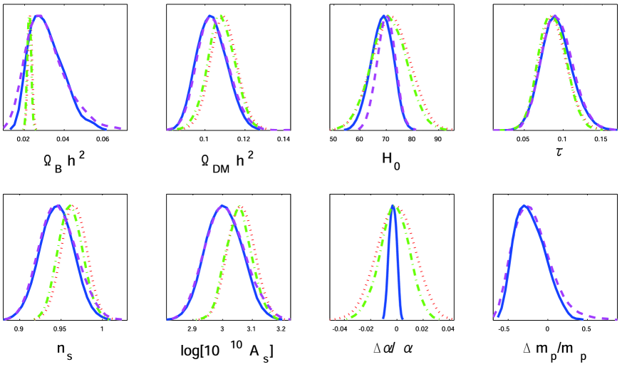
Figure 2: One-dimensional marginalized posterior distributions for four models: varying all three constants α,me𝛼subscript𝑚𝑒\alpha,m_{e} and mpsubscript𝑚𝑝m_{p} assuming the relation (16) and (17) (solid blue curves), varying only two constants α𝛼\alpha and mesubscript𝑚𝑒m_{e} assuming the relation (17) (dot-dashed green curves), varying only one constant α𝛼\alpha (dotted red curves) and varying only one constant mpsubscript𝑚𝑝m_{p} (dashed magenta curves).
Table 1: MCMC results on the mean values and 68%percent\% confidence intervals of cosmological parameters for four versions: varying α𝛼\alpha only, varying α𝛼\alpha and mesubscript𝑚𝑒m_{e}, varying α,me𝛼subscript𝑚𝑒\alpha,m_{e} and mpsubscript𝑚𝑝m_{p}, varying mpsubscript𝑚𝑝m_{p} only.
varying α𝛼\alpha only varying α𝛼\alpha and mesubscript𝑚𝑒m_{e}   varying α,me𝛼subscript𝑚𝑒\alpha,m_{e} and mpsubscript𝑚𝑝m_{p}    varying mpsubscript𝑚𝑝m_{p} only
100ΩBh2100subscriptΩ𝐵superscript2100\Omega_{B}h^{2} 2.270.10+0.10subscriptsuperscript2.270.100.102.27^{+0.10}_{-0.10} 2.240.09+0.09subscriptsuperscript2.240.090.092.24^{+0.09}_{-0.09}   3.130.83+0.85subscriptsuperscript3.130.850.833.13^{+0.85}_{-0.83}    3.130.95+0.97subscriptsuperscript3.130.970.953.13^{+0.97}_{-0.95}
ΩDMh2subscriptΩ𝐷𝑀superscript2\Omega_{DM}h^{2} 0.1090.006+0.006subscriptsuperscript0.1090.0060.0060.109^{+0.006}_{-0.006} 0.1080.006+0.007subscriptsuperscript0.1080.0070.0060.108^{+0.007}_{-0.006}   0.1030.007+0.008subscriptsuperscript0.1030.0080.0070.103^{+0.008}_{-0.007}    0.1040.007+0.007subscriptsuperscript0.1040.0070.0070.104^{+0.007}_{-0.007}
τ𝜏\tau 0.08770.008+0.007subscriptsuperscript0.08770.0070.0080.0877^{+0.007}_{-0.008} 0.08640.009+0.008subscriptsuperscript0.08640.0080.0090.0864^{+0.008}_{-0.009}   0.09160.010+0.007subscriptsuperscript0.09160.0070.0100.0916^{+0.007}_{-0.010}    0.09280.010+0.008subscriptsuperscript0.09280.0080.0100.0928^{+0.008}_{-0.010}
nssubscript𝑛𝑠n_{s} 0.9660.015+0.014subscriptsuperscript0.9660.0140.0150.966^{+0.014}_{-0.015} 0.9610.015+0.014subscriptsuperscript0.9610.0140.0150.961^{+0.014}_{-0.015}   0.9450.020+0.020subscriptsuperscript0.9450.0200.0200.945^{+0.020}_{-0.020}    0.9470.022+0.022subscriptsuperscript0.9470.0220.0220.947^{+0.022}_{-0.022}
log(1010As)superscript1010subscript𝐴𝑠\log(10^{10}A_{s}) 3.060.04+0.05subscriptsuperscript3.060.050.043.06^{+0.05}_{-0.04} 3.060.04+0.04subscriptsuperscript3.060.040.043.06^{+0.04}_{-0.04}   3.000.06+0.06subscriptsuperscript3.000.060.063.00^{+0.06}_{-0.06}    3.010.07+0.06subscriptsuperscript3.010.060.073.01^{+0.06}_{-0.07}
H0subscript𝐻0H_{0} 71.97.1+7.0subscriptsuperscript71.97.07.171.9^{+7.0}_{-7.1} 71.06.4+6.4subscriptsuperscript71.06.46.471.0^{+6.4}_{-6.4}   68.24.2+4.2subscriptsuperscript68.24.24.268.2^{+4.2}_{-4.2}    69.93.4+3.3subscriptsuperscript69.93.33.469.9^{+3.3}_{-3.4}
 
Δα/αΔ𝛼𝛼\Delta\alpha/\alpha 0.000890.0148+0.0131subscriptsuperscript0.000890.01310.0148-0.00089^{+0.0131}_{-0.0148} 0.00190.011+0.011subscriptsuperscript0.00190.0110.011-0.0019^{+0.011}_{-0.011}   0.00310.0029+0.0028subscriptsuperscript0.00310.00280.0029-0.0031^{+0.0028}_{-0.0029}   
 
Δmp/mpΔsubscript𝑚𝑝subscript𝑚𝑝\Delta m_{p}/m_{p}   0.220.19+0.19subscriptsuperscript0.220.190.19-0.22^{+0.19}_{-0.19}    0.190.23+0.22subscriptsuperscript0.190.220.23-0.19^{+0.22}_{-0.23}

Based on the model described in the previous section, we constrain the variation of α𝛼\alpha using three kinds of CMB anisotropy spectra, CTTsuperscriptsubscript𝐶𝑇𝑇C_{\ell}^{TT}, CEEsuperscriptsubscript𝐶𝐸𝐸C_{\ell}^{EE}, and CTEsuperscriptsubscript𝐶𝑇𝐸C_{\ell}^{TE} of the five-year WMAP data Nolta:2008ih ; Dunkley:2008ie ; Komatsu:2008hk . Theoretical anisotropy spectra are calculated by the CAMB code Lewis:1999bs ; camb modified to include the varying physical constants as in Sec. II. We performed the parameter estimation using Markov-Chain Monte-Carlo (MCMC) techniques implemented in the public CosmoMC code Lewis:2002ah ; cosmomc .

We have run the CosmoMC code on eight Markov chains in each case. To check the convergence, we used the “variance of chain means”/“mean of chain variances” R𝑅R statistic and adopted the condition R1<0.03𝑅10.03R-1<0.03. In all the analysis below, we have also incorporated the result of Hubble Key Project of the Hubble Space Telescope (HST) on the Hubble parameter H0subscript𝐻0H_{0}, which means that we have imposed Gaussian prior of H0=72±8kmsec1Mpc1subscript𝐻0plus-or-minus728kmsuperscriptsec1superscriptMpc1H_{0}=72\pm 8\,\mathrm{km\ sec^{-1}\ Mpc^{-1}} Freedman:2000cf . In our analysis, we derive the confidence limits for standard parameters (ΩBh2,ΩDMh2,H0,ns,As,τ)subscriptΩ𝐵superscript2subscriptΩ𝐷𝑀superscript2subscript𝐻0subscript𝑛𝑠subscript𝐴𝑠𝜏(\Omega_{B}h^{2},\Omega_{DM}h^{2},H_{0},n_{s},A_{s},\tau) plus some varying physical constants.

Figures 2 show 1D-marginalized posterior distributions of the eight parameters for the case not only α𝛼\alpha but also mesubscript𝑚𝑒m_{e} and mpsubscript𝑚𝑝m_{p} are changed simultaneously according to the model described in the previous section. This is the main result of this paper and for comparison with the literature we have also plotted the distributions for two other cases: the case of varying only α𝛼\alpha Nakashima:2008cb and the case of varying both α𝛼\alpha and mesubscript𝑚𝑒m_{e} assuming the relation (17) which has already been analyzed in Scoccola:2008jw . In TABLE 1, we also present the mean values and the 68%percent\% confidence intervals of the cosmological parameters for these three cases. We can conclude from these results that the inclusion of the variation of mpsubscript𝑚𝑝m_{p} results in a tighter limit on the variation of α𝛼\alpha, which is now

8.28×10³<Δαα<1.81×103,8.28superscript103Δ𝛼𝛼1.81superscript103-8.28\times 10^{-3}<\frac{\Delta\alpha}{\alpha}<1.81\times 10^{-3}, (18)

compared with the limit for the two other cases: 0.024<Δα/α<0.0190.024Δ𝛼𝛼0.019-0.024<\Delta\alpha/\alpha<0.019 (for varying α,me𝛼subscript𝑚𝑒\alpha,m_{e}) and 0.028<Δα/α<0.0260.028Δ𝛼𝛼0.026-0.028<\Delta\alpha/\alpha<0.026 (for vayring only α𝛼\alpha), all of which are at 95%percent\%C.L.

Refer to caption
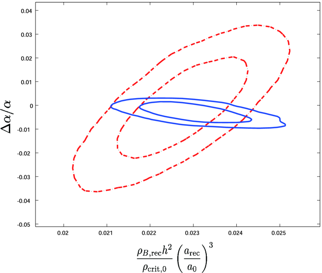
Figure 3: Two-dimensional marginalized posterior distributions of ρB,rech2/ρcrit,0subscript𝜌𝐵recsuperscript2subscript𝜌crit0\rho_{B,\mathrm{rec}}h^{2}/\rho_{\mathrm{crit,0}} and Δα/αΔ𝛼𝛼\Delta\alpha/\alpha for two models: varying all three constants α,me𝛼subscript𝑚𝑒\alpha,m_{e} and mpsubscript𝑚𝑝m_{p} assuming the relation (16) and (17) (solid blue contours) and varying only one constant α𝛼\alpha (dot-dashed red contours). The plotted ρB,rech2/ρcrit,0subscript𝜌𝐵recsuperscript2subscript𝜌crit0\rho_{B,\mathrm{rec}}h^{2}/\rho_{\mathrm{crit,0}} (horizontal axis) is actually (ρB,rech2/ρcrit,0)(arec/a0)3subscript𝜌𝐵recsuperscript2subscript𝜌crit0superscriptsubscript𝑎recsubscript𝑎03(\rho_{B,\mathrm{rec}}h^{2}/\rho_{\mathrm{crit,0}})(a_{\mathrm{rec}}/a_{\mathrm{0}})^{3}, which corresponds to (ρB,0h2/ρcrit,0)(1+Δmp/mp)subscript𝜌𝐵0superscript2subscript𝜌crit01Δsubscript𝑚𝑝subscript𝑚𝑝(\rho_{B,\mathrm{0}}h^{2}/\rho_{\mathrm{crit,0}})(1+\Delta m_{p}/m_{p}) for the former case and ρB,0h2/ρcrit,0subscript𝜌𝐵0superscript2subscript𝜌crit0\rho_{B,\mathrm{0}}h^{2}/\rho_{\mathrm{crit,0}} for the latter case. In each pair of contours, the inner one shows 68%percent\%C.L. and the outer one shows 95%percent\%C.L.

In FIG. 2 and TABLE 1, we can also see that, as a cost of tightening of the constraint on α𝛼\alpha, the limit on ΩBh2subscriptΩ𝐵superscript2\Omega_{B}h^{2}, which is one of the most tightly constrained parameter from CMB data in ordinary analysis, become very loose because of the degeneracy between ΩBsubscriptΩ𝐵\Omega_{B} and Δmp/mpΔsubscript𝑚𝑝subscript𝑚𝑝\Delta m_{p}/m_{p}. This result is reasonable from the argument in Sec. II. On the other hand, since CMB is sensitive to the values of cosmological parameters at the recombination epoch, the limit on ΩB,recsubscriptΩ𝐵rec\Omega_{B,\mathrm{rec}} in the present scenario is expected to be of the same order as that on ΩB,recsubscriptΩ𝐵rec\Omega_{B,\mathrm{rec}} in the case without mpsubscript𝑚𝑝m_{p} variation. We can confirm it from FIG. 3, which shows 2D-marginalized posterior distributions of Δα/αΔ𝛼𝛼\Delta\alpha/\alphaρB,rech2/ρcrit,0subscript𝜌𝐵recsuperscript2subscript𝜌crit0\rho_{B,\mathrm{rec}}h^{2}/\rho_{\mathrm{crit,0}} for two cases, one with both mpsubscript𝑚𝑝m_{p} and mesubscript𝑚𝑒m_{e} variation and the other with no variation in mpsubscript𝑚𝑝m_{p} and mesubscript𝑚𝑒m_{e}.

One of the reasons why we could obtain tighter constraint than the case without varying mpsubscript𝑚𝑝m_{p} is thought to be the specific relation (16) in our model. To ensure that statement, we have also implemented MCMC calculations in the case that only mpsubscript𝑚𝑝m_{p} is varied and the other two physical constants remain constant, which means that we do not impose any model in this case. The result is also shown in FIG. 2 as 1D-marginalized posterior distributions. Two marginalized curves in the panel showing Δmp/mpΔsubscript𝑚𝑝subscript𝑚𝑝\Delta m_{p}/m_{p} are very similar and those limits at 95%percent\%C.L. are 0.54<Δmp/mp<0.360.54Δsubscript𝑚𝑝subscript𝑚𝑝0.36-0.54<\Delta m_{p}/m_{p}<0.36 (for varying mpsubscript𝑚𝑝m_{p} only) and 0.51<Δmp/mp<0.170.51Δsubscript𝑚𝑝subscript𝑚𝑝0.17-0.51<\Delta m_{p}/m_{p}<0.17 (for varying α,me𝛼subscript𝑚𝑒\alpha,m_{e} and mpsubscript𝑚𝑝m_{p}), which implies that the dominant factor in constraining the variation of physical constants under the relation (17) and (16) is Δmp/mpΔsubscript𝑚𝑝subscript𝑚𝑝\Delta m_{p}/m_{p} and it is the specific relation between Δα/αΔ𝛼𝛼\Delta\alpha/\alpha and Δmp/mpΔsubscript𝑚𝑝subscript𝑚𝑝\Delta m_{p}/m_{p} that determines the order of magnitude of the resultant Δα/αΔ𝛼𝛼\Delta\alpha/\alpha limit in the case these parameters are varied simultaneously through the dilaton’s motion.
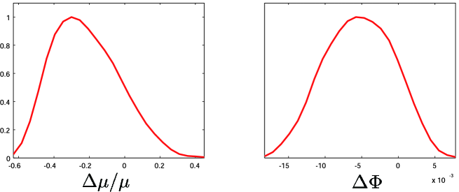
Refer to caption
Figure 4: One-dimensional marginalized posterior distributions for two parameters: Δμ/μΔ𝜇𝜇\Delta\mu/\mu and ΔΦΔΦ\Delta\Phi

Finally, in our model, we can calculate the limit on not only Δα/αΔ𝛼𝛼\Delta\alpha/\alpha but also ΔΦΔΦ\Delta\Phi and Δμ/μΔ𝜇𝜇\Delta\mu/\mu where μmp/me𝜇subscript𝑚𝑝subscript𝑚𝑒\mu\equiv m_{p}/m_{e}. The results are shown in FIG. 4. ΔΦΔΦ\Delta\Phi is the dilaton field variation and using the relation (14) with κ=8πG=(2.43×10¹⁸[GeV])1𝜅8𝜋𝐺superscript2.43superscript1018delimited-[]GeV1\kappa=\sqrt{8\pi G}=(2.43\times 10^{18}[\mathrm{GeV}])^{-1}, we obtain at 95%percent\%C.L.

1.4×10¹⁶[GeV]<ΔΦ<3.1×10¹⁵[GeV].1.4superscript1016delimited-[]GeVΔΦ3.1superscript1015delimited-[]GeV-1.4\times 10^{16}[\mathrm{GeV}]<\Delta\Phi<3.1\times 10^{15}[\mathrm{GeV}]. (19)

On the other hand, the constraint on Δμ/μΔ𝜇𝜇\Delta\mu/\mu is, at 95%percent\%C.L.,

0.52<Δμμ<0.17.0.52Δ𝜇𝜇0.17-0.52<\frac{\Delta\mu}{\mu}<0.17. (20)

Note that, although it is not so stringent compared with those obtained from other experiments Reinhold:2006zn , constraining this parameter in the recombination epoch is meaningful because in the previous works the variation of mpsubscript𝑚𝑝m_{p} has never been considered. We also expect that future CMB measurement such as PLANCK will give more stringent limits of these parameters (see Appendix B).

V Conclusion

In summary, we have pointed out that the time variation of ΛQCDsubscriptΛQCD\Lambda_{\mathrm{QCD}} can affect the CMB through the variation in the proton mass. We have shown that there is a notable effect when we impose the widely adopted assumptions of unification models found in the literature Campbell:1994bf . From the WMAP 5-year data, by MCMC analysis using the CosmoMC code, we have obtained the new and stringent constraint on the time variation of the fine structure constant as 8.28×10³<Δα/α<1.81×1038.28superscript103Δ𝛼𝛼1.81superscript103-8.28\times 10^{-3}<\Delta\alpha/\alpha<1.81\times 10^{-3}. We have also verified that, in getting the above result, the newly considered effect of Δmp/mpΔsubscript𝑚𝑝subscript𝑚𝑝\Delta m_{p}/m_{p} is very important in that the degeneracy between Δmp/mpΔsubscript𝑚𝑝subscript𝑚𝑝\Delta m_{p}/m_{p} and ΩBsubscriptΩ𝐵\Omega_{B} is tremendously strong and that the small variation of Δα/αΔ𝛼𝛼\Delta\alpha/\alpha leads to the large variation of Δmp/mpΔsubscript𝑚𝑝subscript𝑚𝑝\Delta m_{p}/m_{p}. Furthermore, by including the varying mpsubscript𝑚𝑝m_{p}, we have obtained a limit on the variation of proton-electron mass ratio μ𝜇\mu as 0.52<Δμ/μ<0.170.52Δ𝜇𝜇0.17-0.52<\Delta\mu/\mu<0.17.

CMB observation will be much more precise to give a lot of information around the damping tail of the power spectrum in near future. The difference in the CMB power spectra between Δmp/mpΔsubscript𝑚𝑝subscript𝑚𝑝\Delta m_{p}/m_{p} and ΩBsubscriptΩ𝐵\Omega_{B} appears in the small scale diffusion damping because the damping scale is determined by the baryon number density nBsubscript𝑛𝐵n_{B}, probing the time variation of coupling constants including ΛQCDsubscriptΛQCD\Lambda_{\mathrm{QCD}} by CMB will be even more promising. This is discussed more quantitatively in appendix A, and supported by a forecast for future CMB survey in appendix B.


Acknowledgements

We would like to thank Asantha Cooray for useful comments and Toyokazu Sekiguchi for useful help. M.N. is supported by JSPS through research fellowships. This work was partially supported by JSPS Grant-in-Aid for Scientific Research No. 19340054 and Global COE Program ”The Physical Sciences Frontier,” MEXT, Japan.

Appendix A

In this appendix, we discuss the degeneracies between cosmological parameters using the linear algebra. In section II, we have introduced four variables 1,H1,H2,H3subscript1subscript𝐻1subscript𝐻2subscript𝐻3\ell_{1},H_{1},H_{2},H_{3} and calculated how they depend on the cosmological parameters and the physical constants (ωb,ωm,h,τ,ns,αrec,me,rec,mp,rec)subscript𝜔𝑏subscript𝜔𝑚𝜏subscript𝑛𝑠subscript𝛼recsubscript𝑚𝑒recsubscript𝑚𝑝rec(\omega_{b},\omega_{m},h,\tau,n_{s},\alpha_{\mathrm{rec}},m_{e,\mathrm{rec}},m_{p,\mathrm{rec}}), the results of which are shown in (6)-(9). These are rewritten in the matrix form as follows.

(Δ11ΔH1H1ΔH2H2ΔH3H3)=(0.0690.1090.2060.16201.4420.6460.0870.4140.4080.2942.6660.0930.6440.1530.1270.6470.04501.18301.6730.4460.7830.4150.43800.76000.9670.0180.567)(ΔωbωbΔωmωmΔhhΔnsnsΔττΔααΔmemeΔmpmp),Δsubscript1subscript1Δsubscript𝐻1subscript𝐻1Δsubscript𝐻2subscript𝐻2Δsubscript𝐻3subscript𝐻30.0690.1090.2060.16201.4420.6460.0870.4140.4080.2942.6660.0930.6440.1530.1270.6470.04501.18301.6730.4460.7830.4150.43800.76000.9670.0180.567Δsubscript𝜔𝑏subscript𝜔𝑏Δsubscript𝜔𝑚subscript𝜔𝑚ΔΔsubscript𝑛𝑠subscript𝑛𝑠Δ𝜏𝜏Δ𝛼𝛼Δsubscript𝑚𝑒subscript𝑚𝑒Δsubscript𝑚𝑝subscript𝑚𝑝\left(\begin{array}[]{c}\frac{\Delta\ell_{1}}{\ell_{1}}\\ \frac{\Delta H_{1}}{H_{1}}\\ \frac{\Delta H_{2}}{H_{2}}\\ \frac{\Delta H_{3}}{H_{3}}\end{array}\right)=\left(\begin{array}[]{cccccccc}0.069&-0.109&-0.206&0.162&0&-1.442&0.646&0.087\\ 0.414&-0.408&-0.294&2.666&-0.093&0.644&0.153&0.127\\ -0.647&-0.045&0&1.183&0&1.673&0.446&-0.783\\ -0.415&0.438&0&0.760&0&0.967&-0.018&-0.567\end{array}\right)\left(\begin{array}[]{c}\frac{\Delta\omega_{b}}{\omega_{b}}\\ \frac{\Delta\omega_{m}}{\omega_{m}}\\ \frac{\Delta h}{h}\\ \frac{\Delta n_{s}}{n_{s}}\\ \frac{\Delta\tau}{\tau}\\ \frac{\Delta\alpha}{\alpha}\\ \frac{\Delta m_{e}}{m_{e}}\\ \frac{\Delta m_{p}}{m_{p}}\\ \end{array}\right), (21)

where we have divided the both sides of each equation by the fiducial values 1=219.9,H1=6.864,H2=0.4482,H3=0.4342formulae-sequencesubscript1219.9formulae-sequencesubscript𝐻16.864formulae-sequencesubscript𝐻20.4482subscript𝐻30.4342\ell_{1}=219.9,H_{1}=6.864,H_{2}=0.4482,H_{3}=0.4342, respectively. The 4×8484\times 8 matrix connects the cosmological parameters and the CMB variables. Such a rectangular n×m𝑛𝑚n\times m matrix, which we call A𝐴A, can be decomposed in general as

A=UΣVT(U:n×n,Σ:n×m,V:m×m),A=U\Sigma V^{\mathrm{T}}\ \ \ (U:n\times n,\ \Sigma:n\times m,\ V:m\times m), (22)

which is known as the singular value decomposition. If n<m𝑛𝑚n<m and rankA=nrank𝐴𝑛\mathrm{rank}A=n, then the form of ΣΣ\Sigma is like

Σ=(σ10σn),Σsubscript𝜎1missing-subexpressionmissing-subexpressionmissing-subexpressionmissing-subexpressionmissing-subexpression0missing-subexpressionmissing-subexpressionsubscript𝜎𝑛missing-subexpression\Sigma=\left(\begin{array}[]{ccc|c}\sigma_{1}&&&\\ &\ddots&&0\\ &&\sigma_{n}&\end{array}\right), (23)

where σisubscript𝜎𝑖\sigma_{i} is the non-zero singular value of the matrix A𝐴A and the matrices U𝑈U and V𝑉V are orthonormal ones. Applying the singular value decomposition to the 4×8484\times 8 matrix in (21) and using the notation D=UΣ𝐷𝑈ΣD=U\Sigma, we obtain

D𝐷\displaystyle D =(0.6721.2270.7940.03300002.4631.3500.3220.00800002.11450.8150.4880.23800001.2680.6140.2320.3980000)absent0.6721.2270.7940.03300002.4631.3500.3220.00800002.11450.8150.4880.23800001.2680.6140.2320.3980000\displaystyle=\left(\begin{array}[]{cccccccc}-0.672&-1.227&-0.794&0.033&0&0&0&0\\ 2.463&-1.350&0.322&0.008&0&0&0&0\\ 2.1145&0.815&-0.488&-0.238&0&0&0&0\\ 1.268&0.614&-0.232&0.398&0&0&0&0\end{array}\right) (28)
VTsuperscript𝑉T\displaystyle V^{\mathrm{T}} =(0.0730.0370.0460.7880.0180.5810.0690.1680.3260.2090.1490.5420.0290.6540.1480.2890.4780.1210.0670.0240.0290.3040.6600.4730.0280.8250.0420.2220.0030.2530.4190.1660.0190.0130.0270.03500.9980.0060.0200.0130.7020.3310.3180.1690.0180.2300.4500.1060.06700.2850.8170.0740.0190.0490.3470.3440.4020.2610.4470.0280.0190.1530.1960.712)absent0.0730.0370.0460.7880.0180.5810.0690.1680.3260.2090.1490.5420.0290.6540.1480.2890.4780.1210.0670.0240.0290.3040.6600.4730.0280.8250.0420.2220.0030.2530.4190.1660.0190.0130.0270.03500.9980.0060.0200.0130.7020.3310.3180.1690.0180.2300.4500.1060.06700.2850.8170.0740.0190.0490.3470.3440.4020.2610.4470.0280.0190.1530.1960.712\displaystyle=\left(\begin{array}[]{cccccccc}-0.073&-0.037&-0.046&0.788&-0.018&0.581&0.069&-0.168\\ -0.326&0.209&0.149&-0.542&0.029&0.654&-0.148&-0.289\\ 0.478&-0.121&0.067&-0.024&-0.029&0.304&-0.660&0.473\\ -0.028&0.825&-0.042&0.222&-0.003&-0.253&-0.419&-0.166\\ 0.019&-0.013&0.027&0.0350&0.998&-0.006&-0.020&0.013\\ 0.702&0.331&-0.318&-0.169&0.018&0.230&0.450&-0.106\\ 0.0670&0.285&0.817&0.074&-0.019&0.049&0.347&0.344\\ -0.402&0.261&-0.447&-0.028&0.019&0.153&0.196&0.712\end{array}\right) (37)

Now, (21) becomes

(Δ11ΔH1H1ΔH2H2ΔH3H3)=DVT(ΔωbωbΔωmωmΔhhΔnsnsΔττΔmpmp)D(0.788Δnsns+0.581Δαα0.542Δnsns+0.654Δαα0.478Δωbωb0.660Δmeme+0.473Δmpmp0.825Δωmωm0.419Δmeme0.999Δττ0.702Δωbωb+0.451Δmeme0.817Δhh0.402Δωbωb0.447Δhh+0.712Δmpmp)Δsubscript1subscript1Δsubscript𝐻1subscript𝐻1Δsubscript𝐻2subscript𝐻2Δsubscript𝐻3subscript𝐻3𝐷superscript𝑉TΔsubscript𝜔𝑏subscript𝜔𝑏Δsubscript𝜔𝑚subscript𝜔𝑚ΔΔsubscript𝑛𝑠subscript𝑛𝑠Δ𝜏𝜏Δsubscript𝑚𝑝subscript𝑚𝑝𝐷0.788Δsubscript𝑛𝑠subscript𝑛𝑠0.581Δ𝛼𝛼0.542Δsubscript𝑛𝑠subscript𝑛𝑠0.654Δ𝛼𝛼0.478Δsubscript𝜔𝑏subscript𝜔𝑏0.660Δsubscript𝑚𝑒subscript𝑚𝑒0.473Δsubscript𝑚𝑝subscript𝑚𝑝0.825Δsubscript𝜔𝑚subscript𝜔𝑚0.419Δsubscript𝑚𝑒subscript𝑚𝑒0.999Δ𝜏𝜏0.702Δsubscript𝜔𝑏subscript𝜔𝑏0.451Δsubscript𝑚𝑒subscript𝑚𝑒0.817Δ0.402Δsubscript𝜔𝑏subscript𝜔𝑏0.447Δ0.712Δsubscript𝑚𝑝subscript𝑚𝑝\left(\begin{array}[]{c}\frac{\Delta\ell_{1}}{\ell_{1}}\\ \frac{\Delta H_{1}}{H_{1}}\\ \frac{\Delta H_{2}}{H_{2}}\\ \frac{\Delta H_{3}}{H_{3}}\end{array}\right)=DV^{\mathrm{T}}\left(\begin{array}[]{c}\frac{\Delta\omega_{b}}{\omega_{b}}\\ \frac{\Delta\omega_{m}}{\omega_{m}}\\ \frac{\Delta h}{h}\\ \frac{\Delta n_{s}}{n_{s}}\\ \frac{\Delta\tau}{\tau}\\ \frac{\Delta m_{p}}{m_{p}}\end{array}\right)\approx D\left(\begin{array}[]{c}0.788\frac{\Delta n_{s}}{n_{s}}+0.581\frac{\Delta\alpha}{\alpha}\\ -0.542\frac{\Delta n_{s}}{n_{s}}+0.654\frac{\Delta\alpha}{\alpha}\\ 0.478\frac{\Delta\omega_{b}}{\omega_{b}}-0.660\frac{\Delta m_{e}}{m_{e}}+0.473\frac{\Delta m_{p}}{m_{p}}\\ 0.825\frac{\Delta\omega_{m}}{\omega_{m}}-0.419\frac{\Delta m_{e}}{m_{e}}\\ 0.999\frac{\Delta\tau}{\tau}\\ -0.702\frac{\Delta\omega_{b}}{\omega_{b}}+0.451\frac{\Delta m_{e}}{m_{e}}\\ 0.817\frac{\Delta h}{h}\\ -0.402\frac{\Delta\omega_{b}}{\omega_{b}}-0.447\frac{\Delta h}{h}+0.712\frac{\Delta m_{p}}{m_{p}}\end{array}\right) (38)

At the last transformation, we have neglected the terms whose coefficients are small and irrelevant. Remembering the explict form of the matrix D𝐷D that the last four columns are zero, the last four components in the column vector represent the four degeneracy directions, 0.999Δτ/τ,0.702Δωb/ωb+0.451Δme/me,0.817Δh/h,0.402Δωb/ωb0.447Δh/h+0.712Δmp/mp0.999Δ𝜏𝜏0.702Δsubscript𝜔𝑏subscript𝜔𝑏0.451Δsubscript𝑚𝑒subscript𝑚𝑒0.817Δ0.402Δsubscript𝜔𝑏subscript𝜔𝑏0.447Δ0.712Δsubscript𝑚𝑝subscript𝑚𝑝0.999\Delta\tau/\tau,-0.702\Delta\omega_{b}/\omega_{b}+0.451\Delta m_{e}/m_{e},0.817\Delta h/h,-0.402\Delta\omega_{b}/\omega_{b}-0.447\Delta h/h+0.712\Delta m_{p}/m_{p}.

In the above case, where all the variations of physical constants are included in the analysis, the final results are complicated and it is difficult to understand the degeneracies cleary. Therefore, we consider simpler cases in order now.

First, we treat only standard cosmological parameters, so (21) is reduced to

(Δ11ΔH1H1ΔH2H2ΔH3H3)=(0.0690.1090.2060.16200.4140.4080.2942.6660.0930.6470.04501.18300.4150.43800.7600)(ΔωbωbΔωmωmΔhhΔnsnsΔττ).Δsubscript1subscript1Δsubscript𝐻1subscript𝐻1Δsubscript𝐻2subscript𝐻2Δsubscript𝐻3subscript𝐻30.0690.1090.2060.1620missing-subexpression0.4140.4080.2942.6660.093missing-subexpression0.6470.04501.1830missing-subexpression0.4150.43800.7600missing-subexpressionΔsubscript𝜔𝑏subscript𝜔𝑏Δsubscript𝜔𝑚subscript𝜔𝑚ΔΔsubscript𝑛𝑠subscript𝑛𝑠Δ𝜏𝜏\left(\begin{array}[]{c}\frac{\Delta\ell_{1}}{\ell_{1}}\\ \frac{\Delta H_{1}}{H_{1}}\\ \frac{\Delta H_{2}}{H_{2}}\\ \frac{\Delta H_{3}}{H_{3}}\end{array}\right)=\left(\begin{array}[]{cccccc}0.069&-0.109&-0.206&0.162&0\\ 0.414&-0.408&-0.294&2.666&-0.093\\ -0.647&-0.045&0&1.183&0\\ -0.415&0.438&0&0.760&0\end{array}\right)\left(\begin{array}[]{c}\frac{\Delta\omega_{b}}{\omega_{b}}\\ \frac{\Delta\omega_{m}}{\omega_{m}}\\ \frac{\Delta h}{h}\\ \frac{\Delta n_{s}}{n_{s}}\\ \frac{\Delta\tau}{\tau}\end{array}\right). (39)

The singular value decomposition of the 4×5454\times 5 matrix gives

D=(0.1900.1310.0520.17202.7130.4200.0390.01701.1710.6260.2390.00600.7080.6090.2610.0310),VT=(0.0090.0940.0900.9910.0270.8790.4430.1570.0660.0410.4520.8880.0050.07870.0280.1410.0750.9820.0800.0530.05600.0430.0310.997),formulae-sequence𝐷0.1900.1310.0520.17202.7130.4200.0390.01701.1710.6260.2390.00600.7080.6090.2610.0310superscript𝑉T0.0090.0940.0900.9910.0270.8790.4430.1570.0660.0410.4520.8880.0050.07870.0280.1410.0750.9820.0800.0530.05600.0430.0310.997D=\left(\begin{array}[]{ccccc}-0.190&0.131&-0.052&-0.172&0\\ -2.713&0.420&0.039&0.017&0\\ -1.171&-0.626&-0.239&0.006&0\\ -0.708&-0.609&0.261&-0.031&0\end{array}\right),V^{\mathrm{T}}=\left(\begin{array}[]{ccccc}-0.009&0.094&0.090&-0.991&0.027\\ 0.879&-0.443&-0.157&-0.066&-0.041\\ 0.452&0.888&-0.005&0.0787&-0.028\\ 0.141&-0.075&0.982&0.080&-0.053\\ 0.056&0&0.043&0.031&0.997\end{array}\right), (40)

and we get the approxmated relation

(Δ11ΔH1H1ΔH2H2ΔH3H3)=DVT(ΔωbωbΔωmωmΔhhΔnsnsΔττ)D(0.991Δnsns0.879Δωbωb0.443Δωmωm0.452Δωbωb+0.888Δωmωm0.983Δhh0.997Δττ).Δsubscript1subscript1Δsubscript𝐻1subscript𝐻1Δsubscript𝐻2subscript𝐻2Δsubscript𝐻3subscript𝐻3𝐷superscript𝑉TΔsubscript𝜔𝑏subscript𝜔𝑏Δsubscript𝜔𝑚subscript𝜔𝑚ΔΔsubscript𝑛𝑠subscript𝑛𝑠Δ𝜏𝜏𝐷0.991Δsubscript𝑛𝑠subscript𝑛𝑠0.879Δsubscript𝜔𝑏subscript𝜔𝑏0.443Δsubscript𝜔𝑚subscript𝜔𝑚0.452Δsubscript𝜔𝑏subscript𝜔𝑏0.888Δsubscript𝜔𝑚subscript𝜔𝑚0.983Δ0.997Δ𝜏𝜏\left(\begin{array}[]{c}\frac{\Delta\ell_{1}}{\ell_{1}}\\ \frac{\Delta H_{1}}{H_{1}}\\ \frac{\Delta H_{2}}{H_{2}}\\ \frac{\Delta H_{3}}{H_{3}}\end{array}\right)=DV^{\mathrm{T}}\left(\begin{array}[]{c}\frac{\Delta\omega_{b}}{\omega_{b}}\\ \frac{\Delta\omega_{m}}{\omega_{m}}\\ \frac{\Delta h}{h}\\ \frac{\Delta n_{s}}{n_{s}}\\ \frac{\Delta\tau}{\tau}\end{array}\right)\approx D\left(\begin{array}[]{c}-0.991\frac{\Delta n_{s}}{n_{s}}\\ 0.879\frac{\Delta\omega_{b}}{\omega_{b}}-0.443\frac{\Delta\omega_{m}}{\omega_{m}}\\ 0.452\frac{\Delta\omega_{b}}{\omega_{b}}+0.888\frac{\Delta\omega_{m}}{\omega_{m}}\\ 0.983\frac{\Delta h}{h}\\ 0.997\frac{\Delta\tau}{\tau}\end{array}\right). (41)

This tells us that the four standard cosmological parameters, ns,ωb,ωmsubscript𝑛𝑠subscript𝜔𝑏subscript𝜔𝑚n_{s},\omega_{b},\omega_{m} and hh can be determined by observing the four variables 1,H1,H2subscript1subscript𝐻1subscript𝐻2\ell_{1},H_{1},H_{2} and H3subscript𝐻3H_{3}, however the optical depth τ𝜏\tau cannot be limited sufficiently, which is the direct consequence of the fact that we cannot tightly constrain τ𝜏\tau only through the temperature anisotropy spectrum.

In the next case, we add one physical constant Δα/αΔ𝛼𝛼\Delta\alpha/\alpha to the parameter vector;

(Δ11ΔH1H1ΔH2H2ΔH3H3)=(0.0690.1090.2060.16201.4420.4140.4080.2942.6660.0930.6440.6470.04501.18301.6730.4150.43800.76000.967)(ΔωbωbΔωmωmΔhhΔnsnsΔττΔαα).Δsubscript1subscript1Δsubscript𝐻1subscript𝐻1Δsubscript𝐻2subscript𝐻2Δsubscript𝐻3subscript𝐻30.0690.1090.2060.16201.4420.4140.4080.2942.6660.0930.6440.6470.04501.18301.6730.4150.43800.76000.967Δsubscript𝜔𝑏subscript𝜔𝑏Δsubscript𝜔𝑚subscript𝜔𝑚ΔΔsubscript𝑛𝑠subscript𝑛𝑠Δ𝜏𝜏Δ𝛼𝛼\left(\begin{array}[]{c}\frac{\Delta\ell_{1}}{\ell_{1}}\\ \frac{\Delta H_{1}}{H_{1}}\\ \frac{\Delta H_{2}}{H_{2}}\\ \frac{\Delta H_{3}}{H_{3}}\end{array}\right)=\left(\begin{array}[]{cccccc}0.069&-0.109&-0.206&0.162&0&-1.442\\ 0.414&-0.408&-0.294&2.666&-0.093&0.644\\ -0.647&-0.045&0&1.183&0&1.673\\ -0.415&0.438&0&0.760&0&0.967\end{array}\right)\left(\begin{array}[]{c}\frac{\Delta\omega_{b}}{\omega_{b}}\\ \frac{\Delta\omega_{m}}{\omega_{m}}\\ \frac{\Delta h}{h}\\ \frac{\Delta n_{s}}{n_{s}}\\ \frac{\Delta\tau}{\tau}\\ \frac{\Delta\alpha}{\alpha}\end{array}\right). (42)

From the singular value decomposition and the relevant approximation, we obtain

D𝐷\displaystyle D =(0.6941.2190.4360.094002.5401.21230.1720.045001.9700.8100.1620.239001.1820.5410.3540.24600)absent0.6941.2190.4360.094002.5401.21230.1720.045001.9700.8100.1620.239001.1820.5410.3540.24600\displaystyle=\left(\begin{array}[]{cccccc}-0.694&-1.219&-0.436&-0.094&0&0\\ 2.540&-1.2123&0.172&0.045&0&0\\ 1.970&0.810&-0.162&-0.239&0&0\\ 1.182&0.541&-0.354&0.246&0&0\end{array}\right) (47)
VTsuperscript𝑉T\displaystyle V^{\mathrm{T}} =(0.0620.0440.0490.8100.0190.5790.3420.2120.1560.5280.0290.7310.7890.4590.1060.2000.0430.3370.5000.8610.0480.0690.0320.0250.05600.0510.0320.9970.0010.0620.0290.9780.1410.0520.125)absent0.0620.0440.0490.8100.0190.5790.3420.2120.1560.5280.0290.7310.7890.4590.1060.2000.0430.3370.5000.8610.0480.0690.0320.0250.05600.0510.0320.9970.0010.0620.0290.9780.1410.0520.125\displaystyle=\left(\begin{array}[]{cccccc}-0.062&-0.044&-0.049&0.810&-0.019&0.579\\ -0.342&0.212&0.156&-0.528&0.029&0.731\\ 0.789&-0.459&0.106&-0.200&-0.043&0.337\\ 0.500&0.861&0.048&0.069&-0.032&0.025\\ 0.056&0&0.051&0.032&0.997&-0.001\\ 0.062&0.029&-0.978&-0.141&0.052&0.125\end{array}\right) (54)

and

(Δ11ΔH1H1ΔH2H2ΔH3H3)=DVT(ΔωbωbΔωmωmΔhhΔnsnsΔττΔαα)D(0.810Δnsns+0.579Δαα0.342Δωbωb0.528Δnsns+0.731Δαα0.789Δωbωb0.459Δωmωm+0.337Δαα0.500Δωbωb+0.861Δωmωm0.997Δττ0.978Δhh).Δsubscript1subscript1Δsubscript𝐻1subscript𝐻1Δsubscript𝐻2subscript𝐻2Δsubscript𝐻3subscript𝐻3𝐷superscript𝑉TΔsubscript𝜔𝑏subscript𝜔𝑏Δsubscript𝜔𝑚subscript𝜔𝑚ΔΔsubscript𝑛𝑠subscript𝑛𝑠Δ𝜏𝜏Δ𝛼𝛼𝐷0.810Δsubscript𝑛𝑠subscript𝑛𝑠0.579Δ𝛼𝛼0.342Δsubscript𝜔𝑏subscript𝜔𝑏0.528Δsubscript𝑛𝑠subscript𝑛𝑠0.731Δ𝛼𝛼0.789Δsubscript𝜔𝑏subscript𝜔𝑏0.459Δsubscript𝜔𝑚subscript𝜔𝑚0.337Δ𝛼𝛼0.500Δsubscript𝜔𝑏subscript𝜔𝑏0.861Δsubscript𝜔𝑚subscript𝜔𝑚0.997Δ𝜏𝜏0.978Δ\left(\begin{array}[]{c}\frac{\Delta\ell_{1}}{\ell_{1}}\\ \frac{\Delta H_{1}}{H_{1}}\\ \frac{\Delta H_{2}}{H_{2}}\\ \frac{\Delta H_{3}}{H_{3}}\end{array}\right)=DV^{\mathrm{T}}\left(\begin{array}[]{c}\frac{\Delta\omega_{b}}{\omega_{b}}\\ \frac{\Delta\omega_{m}}{\omega_{m}}\\ \frac{\Delta h}{h}\\ \frac{\Delta n_{s}}{n_{s}}\\ \frac{\Delta\tau}{\tau}\\ \frac{\Delta\alpha}{\alpha}\end{array}\right)\approx D\left(\begin{array}[]{c}0.810\frac{\Delta n_{s}}{n_{s}}+0.579\frac{\Delta\alpha}{\alpha}\\ -0.342\frac{\Delta\omega_{b}}{\omega_{b}}-0.528\frac{\Delta n_{s}}{n_{s}}+0.731\frac{\Delta\alpha}{\alpha}\\ 0.789\frac{\Delta\omega_{b}}{\omega_{b}}-0.459\frac{\Delta\omega_{m}}{\omega_{m}}+0.337\frac{\Delta\alpha}{\alpha}\\ 0.500\frac{\Delta\omega_{b}}{\omega_{b}}+0.861\frac{\Delta\omega_{m}}{\omega_{m}}\\ 0.997\frac{\Delta\tau}{\tau}\\ -0.978\frac{\Delta h}{h}\end{array}\right). (55)

The last equation (55) makes a contrast with (41). The newly included parameter Δα/αΔ𝛼𝛼\Delta\alpha/\alpha is now determined together with nssubscript𝑛𝑠n_{s}, ωbsubscript𝜔𝑏\omega_{b} and ωmsubscript𝜔𝑚\omega_{m}, on the other hand the Hubble parameter hh becomes the unlimited parameter like τ𝜏\tau. This is exactly what is expected because in the previous paper Nakashima:2008cb we have made sure that, in constraining Δα/αΔ𝛼𝛼\Delta\alpha/\alpha, the HST prior on the Hubble parameter is very useful, which implied that including Δα/αΔ𝛼𝛼\Delta\alpha/\alpha in the analysis weakens the constraint on hh.

As the third case, which we are most interested in, we add the new parameter Δmp/mpΔsubscript𝑚𝑝subscript𝑚𝑝\Delta m_{p}/m_{p};

(Δ11ΔH1H1ΔH2H2ΔH3H3)=(0.0690.1090.2060.16200.0870.4140.4080.2942.6660.0930.1270.6470.04501.18300.7830.4150.43800.76000.567)(ΔωbωbΔωmωmΔhhΔnsnsΔττΔmpmp).Δsubscript1subscript1Δsubscript𝐻1subscript𝐻1Δsubscript𝐻2subscript𝐻2Δsubscript𝐻3subscript𝐻30.0690.1090.2060.16200.0870.4140.4080.2942.6660.0930.1270.6470.04501.18300.7830.4150.43800.76000.567Δsubscript𝜔𝑏subscript𝜔𝑏Δsubscript𝜔𝑚subscript𝜔𝑚ΔΔsubscript𝑛𝑠subscript𝑛𝑠Δ𝜏𝜏Δsubscript𝑚𝑝subscript𝑚𝑝\left(\begin{array}[]{c}\frac{\Delta\ell_{1}}{\ell_{1}}\\ \frac{\Delta H_{1}}{H_{1}}\\ \frac{\Delta H_{2}}{H_{2}}\\ \frac{\Delta H_{3}}{H_{3}}\end{array}\right)=\left(\begin{array}[]{cccccc}0.069&-0.109&-0.206&0.162&0&0.087\\ 0.414&-0.408&-0.294&2.666&-0.093&0.127\\ -0.647&-0.045&0&1.183&0&-0.783\\ -0.415&0.438&0&0.760&0&-0.567\end{array}\right)\left(\begin{array}[]{c}\frac{\Delta\omega_{b}}{\omega_{b}}\\ \frac{\Delta\omega_{m}}{\omega_{m}}\\ \frac{\Delta h}{h}\\ \frac{\Delta n_{s}}{n_{s}}\\ \frac{\Delta\tau}{\tau}\\ \frac{\Delta m_{p}}{m_{p}}\end{array}\right). (56)

Similar decomposition and approximation lead to

D𝐷\displaystyle D =(0.1770.1700.0560.172002.6760.6290.03050.017001.2600.8900.2300.006000.7760.7630.2810.03100)absent0.1770.1700.0560.172002.6760.6290.03050.017001.2600.8900.2300.006000.7760.7630.2810.03100\displaystyle=\left(\begin{array}[]{cccccc}-0.177&0.170&-0.056&0.172&0&0\\ -2.676&0.629&0.0305&-0.017&0&0\\ -1.260&-0.890&-0.230&-0.006&0&0\\ -0.776&-0.763&0.281&0.031&0&0\end{array}\right) (61)
VTsuperscript𝑉T\displaystyle V^{\mathrm{T}} =(0.0020.0880.0880.9850.0270.1140.6470.3160.1220.0400.0330.6810.3010.9360.01900.1020.02100.1450.1390.0750.9830.0800.0530.0020.03800.0030.0460.0330.9970.0190.6850.0980.0950.0980.0040.709)absent0.0020.0880.0880.9850.0270.1140.6470.3160.1220.0400.0330.6810.3010.9360.01900.1020.02100.1450.1390.0750.9830.0800.0530.0020.03800.0030.0460.0330.9970.0190.6850.0980.0950.0980.0040.709\displaystyle=\left(\begin{array}[]{cccccc}0.002&0.088&0.088&-0.985&0.027&0.114\\ 0.647&-0.316&-0.122&0.040&-0.033&0.681\\ 0.301&0.936&0.0190&0.102&-0.0210&0.145\\ -0.139&0.075&-0.983&-0.080&0.053&-0.002\\ 0.0380&0.003&0.046&0.033&0.997&0.019\\ -0.685&0.098&0.095&0.098&0.004&0.709\end{array}\right) (68)

and

(Δ11ΔH1H1ΔH2H2ΔH3H3)=DVT(ΔωbωbΔωmωmΔhhΔnsnsΔττΔmpmp)D(0.985Δnsns0.647Δωbωb+0.681Δmpmp0.936Δωmωm0.983Δhh0.997Δττ0.685Δωbωb+0.709Δmpmp).Δsubscript1subscript1Δsubscript𝐻1subscript𝐻1Δsubscript𝐻2subscript𝐻2Δsubscript𝐻3subscript𝐻3𝐷superscript𝑉TΔsubscript𝜔𝑏subscript𝜔𝑏Δsubscript𝜔𝑚subscript𝜔𝑚ΔΔsubscript𝑛𝑠subscript𝑛𝑠Δ𝜏𝜏Δsubscript𝑚𝑝subscript𝑚𝑝𝐷0.985Δsubscript𝑛𝑠subscript𝑛𝑠0.647Δsubscript𝜔𝑏subscript𝜔𝑏0.681Δsubscript𝑚𝑝subscript𝑚𝑝0.936Δsubscript𝜔𝑚subscript𝜔𝑚0.983Δ0.997Δ𝜏𝜏0.685Δsubscript𝜔𝑏subscript𝜔𝑏0.709Δsubscript𝑚𝑝subscript𝑚𝑝\left(\begin{array}[]{c}\frac{\Delta\ell_{1}}{\ell_{1}}\\ \frac{\Delta H_{1}}{H_{1}}\\ \frac{\Delta H_{2}}{H_{2}}\\ \frac{\Delta H_{3}}{H_{3}}\end{array}\right)=DV^{\mathrm{T}}\left(\begin{array}[]{c}\frac{\Delta\omega_{b}}{\omega_{b}}\\ \frac{\Delta\omega_{m}}{\omega_{m}}\\ \frac{\Delta h}{h}\\ \frac{\Delta n_{s}}{n_{s}}\\ \frac{\Delta\tau}{\tau}\\ \frac{\Delta m_{p}}{m_{p}}\end{array}\right)\approx D\left(\begin{array}[]{c}-0.985\frac{\Delta n_{s}}{n_{s}}\\ -0.647\frac{\Delta\omega_{b}}{\omega_{b}}+0.681\frac{\Delta m_{p}}{m_{p}}\\ 0.936\frac{\Delta\omega_{m}}{\omega_{m}}\\ -0.983\frac{\Delta h}{h}\\ 0.997\frac{\Delta\tau}{\tau}\\ -0.685\frac{\Delta\omega_{b}}{\omega_{b}}+0.709\frac{\Delta m_{p}}{m_{p}}\end{array}\right). (69)

It is found that there are two degeneracy directions and one of them is 0.685Δωb/ωb+0.709Δmp/mp0.685Δsubscript𝜔𝑏subscript𝜔𝑏0.709Δsubscript𝑚𝑝subscript𝑚𝑝-0.685\Delta\omega_{b}/\omega_{b}+0.709\Delta m_{p}/m_{p}. This means that ωbsubscript𝜔𝑏\omega_{b} and mpsubscript𝑚𝑝m_{p} are strongly degenerate, which could be naively expected from just comparing the coefficients of the two parameters Δωb/ωbΔsubscript𝜔𝑏subscript𝜔𝑏\Delta\omega_{b}/\omega_{b} and Δmp/mpΔsubscript𝑚𝑝subscript𝑚𝑝\Delta m_{p}/m_{p}.

Now, we include the small scale information in the analysis to study how the damping tail is crucial for parameter determination from CMB in the third case. We make use of H4subscript𝐻4H_{4} and H5subscript𝐻5H_{5}, which is defined in the same way as H2,H3subscript𝐻2subscript𝐻3H_{2},H_{3}, that is,

H4(ΔT4ΔT1)2,H5(ΔT5ΔT1)2.formulae-sequencesubscript𝐻4superscriptΔsubscript𝑇subscript4Δsubscript𝑇subscript12subscript𝐻5superscriptΔsubscript𝑇subscript5Δsubscript𝑇subscript12H_{4}\equiv\left(\frac{\Delta T_{\ell_{4}}}{\Delta T_{\ell_{1}}}\right)^{2},\ \ H_{5}\equiv\left(\frac{\Delta T_{\ell_{5}}}{\Delta T_{\ell_{1}}}\right)^{2}. (70)

In other words, H4subscript𝐻4H_{4} is the ratio of the fourth peak 4subscript4\ell_{4} to the first peak 1subscript1\ell_{1} height and H5subscript𝐻5H_{5} is the ratio of the fifth peak 5subscript5\ell_{5} to the first peak 1subscript1\ell_{1}. Adding the relations between ΔH4/H4,ΔH5/H5Δsubscript𝐻4subscript𝐻4Δsubscript𝐻5subscript𝐻5\Delta H_{4}/H_{4},\Delta H_{5}/H_{5} and the variations of the cosmological parameters, (56) becomes

(Δ11ΔH1H1ΔH2H2ΔH3H3ΔH4H4ΔH5H5)=(0.0690.1090.2060.16200.0870.4140.4080.2942.6660.0930.1270.6470.04501.18300.7830.4150.43800.76000.5670.4780.31501.60800.8680.6650.49301.82800.794)(ΔωbωbΔωmωmΔhhΔnsnsΔττΔmpmp).Δsubscript1subscript1Δsubscript𝐻1subscript𝐻1Δsubscript𝐻2subscript𝐻2Δsubscript𝐻3subscript𝐻3Δsubscript𝐻4subscript𝐻4Δsubscript𝐻5subscript𝐻50.0690.1090.2060.16200.0870.4140.4080.2942.6660.0930.1270.6470.04501.18300.7830.4150.43800.76000.5670.4780.31501.60800.8680.6650.49301.82800.794Δsubscript𝜔𝑏subscript𝜔𝑏Δsubscript𝜔𝑚subscript𝜔𝑚ΔΔsubscript𝑛𝑠subscript𝑛𝑠Δ𝜏𝜏Δsubscript𝑚𝑝subscript𝑚𝑝\left(\begin{array}[]{c}\frac{\Delta\ell_{1}}{\ell_{1}}\\ \frac{\Delta H_{1}}{H_{1}}\\ \frac{\Delta H_{2}}{H_{2}}\\ \frac{\Delta H_{3}}{H_{3}}\\ \frac{\Delta H_{4}}{H_{4}}\\ \frac{\Delta H_{5}}{H_{5}}\end{array}\right)=\left(\begin{array}[]{cccccc}0.069&-0.109&-0.206&0.162&0&0.087\\ 0.414&-0.408&-0.294&2.666&-0.093&0.127\\ -0.647&-0.045&0&1.183&0&-0.783\\ -0.415&0.438&0&0.760&0&-0.567\\ -0.478&0.315&0&1.608&0&-0.868\\ 0.665&0.493&0&1.828&0&-0.794\end{array}\right)\left(\begin{array}[]{c}\frac{\Delta\omega_{b}}{\omega_{b}}\\ \frac{\Delta\omega_{m}}{\omega_{m}}\\ \frac{\Delta h}{h}\\ \frac{\Delta n_{s}}{n_{s}}\\ \frac{\Delta\tau}{\tau}\\ \frac{\Delta m_{p}}{m_{p}}\end{array}\right). (71)

We can recast this equation through the relevant approxmation in

(Δ11ΔH1H1ΔH2H2ΔH3H3ΔH4H4ΔH5H5)(0.13780.1980.0850.0120.1650.0012.5281.0240.3430.0420.0230.0011.3320.6800.4090.1700.0130.0030.8970.6480.0270.1940.0140.0041.7850.6840.1040.04690.0120.0062.0070.0460.7890.0690.0130.001)(0.960Δnsns0.617Δωbωb0.658Δmpmp0.734Δωbωb0.579Δωmωm0.728Δωmωm0.582Δmpmp0.959Δhh0.994Δττ).Δsubscript1subscript1Δsubscript𝐻1subscript𝐻1Δsubscript𝐻2subscript𝐻2Δsubscript𝐻3subscript𝐻3Δsubscript𝐻4subscript𝐻4Δsubscript𝐻5subscript𝐻50.13780.1980.0850.0120.1650.0012.5281.0240.3430.0420.0230.0011.3320.6800.4090.1700.0130.0030.8970.6480.0270.1940.0140.0041.7850.6840.1040.04690.0120.0062.0070.0460.7890.0690.0130.0010.960Δsubscript𝑛𝑠subscript𝑛𝑠0.617Δsubscript𝜔𝑏subscript𝜔𝑏0.658Δsubscript𝑚𝑝subscript𝑚𝑝0.734Δsubscript𝜔𝑏subscript𝜔𝑏0.579Δsubscript𝜔𝑚subscript𝜔𝑚0.728Δsubscript𝜔𝑚subscript𝜔𝑚0.582Δsubscript𝑚𝑝subscript𝑚𝑝0.959Δ0.994Δ𝜏𝜏\left(\begin{array}[]{c}\frac{\Delta\ell_{1}}{\ell_{1}}\\ \frac{\Delta H_{1}}{H_{1}}\\ \frac{\Delta H_{2}}{H_{2}}\\ \frac{\Delta H_{3}}{H_{3}}\\ \frac{\Delta H_{4}}{H_{4}}\\ \frac{\Delta H_{5}}{H_{5}}\end{array}\right)\approx\left(\begin{array}[]{cccccc}0.1378&-0.198&0.085&-0.012&-0.165&0.001\\ 2.528&-1.024&0.343&-0.042&0.023&-0.001\\ 1.332&0.680&0.409&0.170&-0.013&-0.003\\ 0.897&0.648&-0.027&-0.194&-0.014&-0.004\\ 1.785&0.684&0.104&-0.0469&0.012&0.006\\ 2.007&-0.046&-0.789&0.069&-0.013&-0.001\end{array}\right)\left(\begin{array}[]{c}0.960\frac{\Delta n_{s}}{n_{s}}\\ -0.617\frac{\Delta\omega_{b}}{\omega_{b}}-0.658\frac{\Delta m_{p}}{m_{p}}\\ -0.734\frac{\Delta\omega_{b}}{\omega_{b}}-0.579\frac{\Delta\omega_{m}}{\omega_{m}}\\ -0.728\frac{\Delta\omega_{m}}{\omega_{m}}-0.582\frac{\Delta m_{p}}{m_{p}}\\ 0.959\frac{\Delta h}{h}\\ 0.994\frac{\Delta\tau}{\tau}\end{array}\right). (72)

All the elements of the last column in 6×6666\times 6 matrix, which correspond to the coefficients of the parameter τ𝜏\tau, are nearly zero, which is almost the same situation occurred in the previous case without ΔH4/H4Δsubscript𝐻4subscript𝐻4\Delta H_{4}/H_{4} and ΔH5/H5Δsubscript𝐻5subscript𝐻5\Delta H_{5}/H_{5}. Unlike the previous case, there are no other (nearly) zero columns, which states that, as mentioned in section V, the strong degeneracy between ωbsubscript𝜔𝑏\omega_{b} and mpsubscript𝑚𝑝m_{p} can be resolved by observing not only 1,H1,H2,H3subscript1subscript𝐻1subscript𝐻2subscript𝐻3\ell_{1},H_{1},H_{2},H_{3} but also H4subscript𝐻4H_{4}, H5subscript𝐻5H_{5} which possess the damping tail information.

Appendix B

In this appendix, we briefly report a forecast for constraints from the future CMB survey, in particular, the PLANCK survey Planck:2006uk . The parameters for the instrumental design for PLANCK survey are shown in TABLE 2 and mock data are generated by the publicly available FuturCMB code Perotto:2006rj . The fiducial parameter values are the same as those adopted in section II and we perform the MCMC analysis in the same way as in section IV. Throughout this appendix, we assume the model between time variations of physical constants introduced in section III.

Table 2: Assumed instrumental parameters for PLANCK survey. fskysubscript𝑓𝑠𝑘𝑦f_{sky} is the fraction of the observed sky, θFWHMsubscript𝜃FWHM\theta_{\mathrm{FWHM}} is Gaussian beam width at FWHM, σTsubscript𝜎𝑇\sigma_{T} and σPsubscript𝜎𝑃\sigma_{P} are temperature and polarization noise, respectively.
fskysubscript𝑓𝑠𝑘𝑦f_{sky} bands[GHz] θFWHM[arcmin]subscript𝜃FWHMdelimited-[]𝑎𝑟𝑐𝑚𝑖𝑛\theta_{\mathrm{FWHM}}[arcmin] σTsubscript𝜎𝑇\sigma_{T}[μ𝜇\muK] σPsubscript𝜎𝑃\sigma_{P}[μ𝜇\muK]
0.65 100 9.5 6.8 10.9
143 7.1 6.0 11.4
217 5.0 13.1 26.7

In TABLE 3, we show the forecast for the constraints on the cosmological parameters as the mean values, 68%percent\% and 95%percent\% confidence intervals. As is commented in the concluding section and appendix A, future CMB survey can constrain time variation of the physical constants more tightly and the limit on Δα/αΔ𝛼𝛼\Delta\alpha/\alpha or Δμ/μΔ𝜇𝜇\Delta\mu/\mu from PLANCK experiment is expected to be about one order tighter than the constraint from the WMAP 5-year data and comparable to the constraint from BBN Ichikawa:2002bt .

Table 3: MCMC results on the mean values, 68%percent\% and 95%percent\% confidence intervals of cosmological parameters.
varying α,me𝛼subscript𝑚𝑒\alpha,m_{e} and mpsubscript𝑚𝑝m_{p}
100ΩBh2100subscriptΩ𝐵superscript2100\Omega_{B}h^{2} 2.2740.0250.049+0.025+0.050subscriptsuperscript2.2740.0250.0500.0250.0492.274^{+0.025+0.050}_{-0.025-0.049}
ΩDMh2subscriptΩ𝐷𝑀superscript2\Omega_{DM}h^{2} 0.1110.0020.003+0.002+0.003subscriptsuperscript0.1110.0020.0030.0020.0030.111^{+0.002+0.003}_{-0.002-0.003}
τ𝜏\tau 0.0870.0030.009+0.002+0.009subscriptsuperscript0.0870.0020.0090.0030.0090.087^{+0.002+0.009}_{-0.003-0.009}
nssubscript𝑛𝑠n_{s} 0.9630.0090.018+0.009+0.017subscriptsuperscript0.9630.0090.0170.0090.0180.963^{+0.009+0.017}_{-0.009-0.018}
log(1010As)superscript1010subscript𝐴𝑠\log(10^{10}A_{s}) 3.0650.0110.023+0.011+0.023subscriptsuperscript3.0650.0110.0230.0110.0233.065^{+0.011+0.023}_{-0.011-0.023}
H0subscript𝐻0H_{0} 71.91.12.0+1.0+2.1subscriptsuperscript71.91.02.11.12.071.9^{+1.0+2.1}_{-1.1-2.0}
Δα/αΔ𝛼𝛼\Delta\alpha/\alpha 0.00000210.00020.0003+0.0002+0.0003subscriptsuperscript0.00000210.00020.00030.00020.00030.0000021^{+0.0002+0.0003}_{-0.0002-0.0003}
Δμ/μΔ𝜇𝜇\Delta\mu/\mu 0.00030.0150.031+0.016+0.030subscriptsuperscript0.00030.0160.0300.0150.0310.0003^{+0.016+0.030}_{-0.015-0.031}

References

  • (1) P. A. M. Dirac, Nature 139 (1937) 323.
  • (2) P. A. M. Dirac, Proc. Roy. Soc. Lond.  A 165 (1938) 199.
  • (3) J. D. Bekenstein, Phys. Rev.  D 25, 1527 (1982).
  • (4) J. D. Barrow, H. B. Sandvik and J. Magueijo, Phys. Rev.  D 65 (2002) 063504 [arXiv:astro-ph/0109414].
  • (5) J. D. Barrow and J. Magueijo, Phys. Rev.  D 72 (2005) 043521 [arXiv:astro-ph/0503222].
  • (6) J. P. Uzan, Rev. Mod. Phys.  75 (2003) 403 [arXiv:hep-ph/0205340].
  • (7) T. Chiba, T. Kobayashi, M. Yamaguchi and J. Yokoyama, Phys. Rev.  D 75 (2007) 043516 [arXiv:hep-ph/0610027].
  • (8) M. Dine and N. Seiberg, Phys. Lett.  B 162 (1985) 299.
  • (9) R. Brustein and P. J. Steinhardt, Phys. Lett.  B 302 (1993) 196 [arXiv:hep-th/9212049].
  • (10) P. P. Avelino, C. J. A. Martins, N. J. Nunes and K. A. Olive, Phys. Rev.  D 74 (2006) 083508 [arXiv:astro-ph/0605690].
  • (11) P. P. Avelino, Phys. Rev.  D 78 (2008) 043516 [arXiv:0804.3394 [astro-ph]].
  • (12) Y. Fujii, Phys. Lett.  B 660 (2008) 87 [arXiv:0709.2211 [astro-ph]].
  • (13) Y. Fujii, Phys. Lett.  B 671 (2009) 207 [arXiv:0809.0411 [astro-ph]].
  • (14) T. Dent, S. Stern and C. Wetterich, JCAP 0901 (2009) 038 [arXiv:0809.4628 [hep-ph]].
  • (15) P. P. Avelino, arXiv:0903.0617 [astro-ph.CO].
  • (16) J. K. Webb, V. V. Flambaum, C. W. Churchill, M. J. Drinkwater and J. D. Barrow, Phys. Rev. Lett.  82 (1999) 884 [arXiv:astro-ph/9803165].
  • (17) J. K. Webb et al., Phys. Rev. Lett.  87 (2001) 091301 [arXiv:astro-ph/0012539].
  • (18) M. T. Murphy et al., Lecture Notes in Phys., 131 (2004), 648.
  • (19) M. T. Murphy, J. K. Webb and V. V. Flambaum, Mon. Not. R. Astron. Soc.  384 (2008), 1053, astro-ph/0612407.
  • (20) M. T. Murphy, J. K. Webb and V. V. Flambaum, Phys. Rev. Lett.  99 (2007), 239001, arXiv:0708.3677.
  • (21) P. Molaro, D. Reimers, I. I. Agafonova and S. A. Levshakov, Eur. Phys. J. ST 163 (2008) 173 [arXiv:0712.4380 [astro-ph]].
  • (22) H. Chand, R. Srianand, P. Petitjean and B. Aracil, Astron. Astrophys.  417 (2004) 853 [arXiv:astro-ph/0401094].
  • (23) R. Srianand, H. Chand, P. Petitjean and B. Aracil, Phys. Rev. Lett.  92 (2004) 121302 [arXiv:astro-ph/0402177].
  • (24) T. Chiba, In Proc. Frontier of Cosmology and Gravitation, (YITP, Kyoto, April 25-27, 2001) [arXiv:gr-qc/0110118].
  • (25) S. Blatt et al., Phys. Rev. Lett.  100 (2008), 140801, arXiv:0801.1874.
  • (26) T. M. Fortier et al., Phys. Rev. Lett.  98 (2007) 070801.
  • (27) E. Peik, B. Lipphardt, H. Schnatz, T. Schneider, C. Tamm and S. G. Karshenboim, Phys. Rev. Lett.  93 (2004) 170801.
  • (28) M. Fischer et al., Phys. Rev. Lett.  92 (2004), 230802.
  • (29) T. Rosenband et al., Science 319 (2008), 1808.
  • (30) Y. Fujii et al., In Proc. Int. Conf. on Nuclear Data for Science and Technology, 2001 [arXiv:hep-ph/0205206].
  • (31) K. Ichikawa and M. Kawasaki, Phys. Rev.  D 65 (2002) 123511 [arXiv:hep-ph/0203006].
  • (32) K. Ichikawa, T. Kanzaki and M. Kawasaki, Phys. Rev.  D 74 (2006) 023515 [arXiv:astro-ph/0602577].
  • (33) G. Rocha, R. Trotta, C. J. A. Martins, A. Melchiorri, P. P. Avelino, R. Bean and P. T. P. Viana, Mon. Not. Roy. Astron. Soc.  352 (2004) 20 [arXiv:astro-ph/0309211].
  • (34) P. Stefanescu, New Astron.  12 (2007) 635 [arXiv:0707.0190 [astro-ph]].
  • (35) M. Nakashima, R. Nagata and J. Yokoyama, Prog. Theor. Phys.  120, 1207 (2008) [arXiv:0810.1098 [astro-ph]].
  • (36) E. Menegoni, S. Galli, J. Bartlett, C. J. A. Martins and A. Melchiorri, arXiv:0909.3584 [astro-ph.CO].
  • (37) E. Reinhold, R. Buning, U. Hollenstein, A. Ivanchik, P. Petitjean and W. Ubachs, Phys. Rev. Lett.  96 (2006) 151101.
  • (38) V. V. Flambaum, M. G. Kozlov and M. G. Kozlov, Phys. Rev. Lett.  98 (2007) 240801 [arXiv:0704.2301 [astro-ph]].
  • (39) M. T. Murphy, V. V. Flambaum, S. Muller and C. Henkel, Science 320 (2008) 1611 [arXiv:0806.3081 [astro-ph]].
  • (40) B. A. Campbell and K. A. Olive, Phys. Lett.  B 345, 429 (1995) [arXiv:hep-ph/9411272].
  • (41) P. Langacker, G. Segre and M. J. Strassler, Phys. Lett.  B 528, 121 (2002) [arXiv:hep-ph/0112233].
  • (42) T. Dent and M. Fairbairn, Nucl. Phys.  B 653 (2003) 256 [arXiv:hep-ph/0112279].
  • (43) C. M. Muller, G. Schafer and C. Wetterich, Phys. Rev.  D 70 (2004) 083504 [arXiv:astro-ph/0405373].
  • (44) T. Dent, S. Stern and C. Wetterich, Phys. Rev.  D 78 (2008) 103518 [arXiv:0808.0702 [hep-ph]].
  • (45) X. Calmet and H. Fritzsch, Eur. Phys. J.  C 24 (2002) 639 [arXiv:hep-ph/0112110].
  • (46) X. Calmet and H. Fritzsch, Phys. Lett.  B 540 (2002) 173 [arXiv:hep-ph/0204258].
  • (47) K. A. Olive, M. Pospelov, Y. Z. Qian, A. Coc, M. Casse and E. Vangioni-Flam, Phys. Rev.  D 66 (2002) 045022 [arXiv:hep-ph/0205269].
  • (48) S. J. Landau, M. E. Mosquera, C. G. Scoccola and H. Vucetich, Phys. Rev.  D 78 (2008) 083527 [arXiv:0809.2033 [astro-ph]].
  • (49) C. G. Scoccola, S. J. Landau and H. Vucetich, Phys. Lett.  B 669 (2008) 212 [arXiv:0809.5028 [astro-ph]].
  • (50) M. Dine, Y. Nir, G. Raz and T. Volansky, Phys. Rev.  D 67 (2003) 015009 [arXiv:hep-ph/0209134].
  • (51) S. Hannestad, Phys. Rev.  D 60 (1999) 023515 [arXiv:astro-ph/9810102].
  • (52) M. Kaplinghat, R. J. Scherrer and M. S. Turner, Phys. Rev.  D 60 (1999) 023516 [arXiv:astro-ph/9810133].
  • (53) J. Kujat and R. J. Scherrer, Phys. Rev.  D 62 (2000) 023510 [arXiv:astro-ph/9912174].
  • (54) J. J. Yoo and R. J. Scherrer, Phys. Rev.  D 67 (2003) 043517 [arXiv:astro-ph/0211545].
  • (55) http://camb.info/
  • (56) J. Dunkley et al. [WMAP Collaboration], Astrophys. J. Suppl.  180 (2009) 306 [arXiv:0803.0586 [astro-ph]].
  • (57) E. Komatsu et al. [WMAP Collaboration], Astrophys. J. Suppl.  180 (2009) 330 [arXiv:0803.0547 [astro-ph]].
  • (58) W. Hu and N. Sugiyama, Astrophys. J.  471 (1996) 542 [arXiv:astro-ph/9510117].
  • (59) W. Hu, M. Fukugita, M. Zaldarriaga and M. Tegmark, Astrophys. J.  549, 669 (2001) [arXiv:astro-ph/0006436].
  • (60) C. Lovelace, Phys. Lett.  B 135 (1984) 75.
  • (61) E. S. Fradkin and A. A. Tseytlin, Phys. Lett.  B 158 (1985) 316.
  • (62) C. G. . Callan, E. J. Martinec, M. J. Perry and D. Friedan, Nucl. Phys.  B 262 (1985) 593.
  • (63) A. Sen, Phys. Rev.  D 32 (1985) 2102.
  • (64) A. Sen, Phys. Rev. Lett.  55 (1985) 1846.
  • (65) C. G. . Callan, I. R. Klebanov and M. J. Perry, Nucl. Phys.  B 278 (1986) 78.
  • (66) M. R. Nolta et al. [WMAP Collaboration], Astrophys. J. Suppl.  180 (2009) 296 [arXiv:0803.0593 [astro-ph]].
  • (67) A. Lewis, A. Challinor and A. Lasenby, Astrophys. J.  538 (2000) 473 [arXiv:astro-ph/9911177].
  • (68) A. Lewis and S. Bridle, Phys. Rev.  D 66 (2002) 103511 [arXiv:astro-ph/0205436].
  • (69) http://cosmologist.info/cosmomc/
  • (70) W. L. Freedman et al. [HST Collaboration], Astrophys. J.  553 (2001) 47 [arXiv:astro-ph/0012376].
  • (71) [Planck Collaboration], arXiv:astro-ph/0604069.
  • (72) L. Perotto, J. Lesgourgues, S. Hannestad, H. Tu and Y. Y. Y. Wong, JCAP 0610 (2006) 013 [arXiv:astro-ph/0606227].