Statistically significant length scale of filaments as a robust measure of galaxy distribution

Abstract

We have used a statistical technique “Shuffle” (Bhavsar & Ling, 1988; Bharadwaj, Bhavsar & Sheth, 2004) in seven nearly two dimensional strips from the Sloan Digital Sky Survey Data Release Six (SDSS DR6) to test if the statistically significant length scale of filaments depends on luminosity, colour and morphology of galaxies. We find that although the average filamentarity depends on these galaxy properties, the statistically significant length scale of filaments does not depend on them. We compare it’s measured values in SDSS against the predictions of $\Lambda$CDM N-body simulations and find that $\Lambda$CDM model is consistent with observations. The average filamentarity is known to be very sensitive to the bias parameter. Using $\Lambda$CDM N-body simulations we simulate mock galaxy distributions for SDSS NGP equatorial strip for different biases and test if the statistically significant length scale of filaments depends on bias. We find that statistically significant length scale of filaments is nearly independent of bias. This result is possibly related to the fact that statistically significant length scale of filaments is nearly the same for different class of galaxies which are differently biased with respect to underlying dark matter distribution. The average filamentarity is also known to be dependent on the galaxy number density and size of the samples. We use $\Lambda$CDM dark matter N-body simulations to test if the statistically significant length scale of filaments depends on number density of galaxies and size of the samples. Our analysis shows that the statistically significant length scale of filaments very weakly depends on these factors. Finally we test the reliability of our method by applying it to controlled samples of segment Cox process and find that our method successfully recovers the length of the inputted segments. Summarizing these results we conclude that the statistically significant length scale of filaments is a robust measure of the galaxy distribution.

1 Introduction

The fact that the galaxies appear to be distributed along filaments which are interconnected to form a web like structure which is often reffered as the ‘cosmic web’ is one of the most striking visual feature in all the present and past redshift surveys (e.g. , CfA , Geller & Huchra 1989; LCRS, Shectman et al. 1996; 2dFGRS, Colles et al. 2001 and SDSS, Stoughton et al. 2002).

The analysis of filamentary patterns in the galaxy distribution has a long history dating back to a few papers in the late-seventies and mid-eighties by Joeveer et al. (1978), Einasto et al. (1980), Zel’dovich , Einasto & Shandarin (1982), Shandarin & Zeldovich (1983) and Einasto et al. (1984). Filaments are the most striking visible patterns seen in the galaxy distribution (e.g. Geller & Huchra 1989, Shectman et al. 1996, Shandarin & Yess 1998, Bharadwaj et al. 2000, Müller et al. 2000, Basilakos, Plionis, & Rowan-Robinson 2001, Doroshkevich et al. 2004, Pimbblet, Drinkwater & Hawkrigg 2004, Pimbblet & Drinkwater 2004, Pandey & Bharadwaj 2005). A review on a number of physically motivated and statistical methods to define filaments is provided in Pimbblet (2005). The percolation analysis (eg. Shandarin & Zeldovich 1983, Einasto et al. 1984), the genus statistics (eg. Gott, Dickinson, & Melott 1986), the minimal spanning tree (e.g. Barrow et al. 1985), the Voronoi tessellation (Icke & van de Weygaert 1987, van de Weygaert & Icke 1989), the Minkowski functionals (eg. Mecke et al. 1994, Schmalzing & Buchert 1997) and the ‘Shapefinders’ (Sahni, Sathyaprakash,& Shandarin, 1998) are some of the useful statistical tools introduced to quantify the topology and geometry of the galaxy distribution. Stoica et al. (2005) propose to apply a marked point process to automatically delineate filaments in the galaxy distribution. Colberg et al. (2005) studied the intercluster filamentary network in high resolution N-body simulations of structure formation in a $\Lambda$CDM Universe. Aragón-Calvo et al. (2007) use Multiscale Morphology Filter technique to identify wall-like and filament-like structures in cosmological N-body simulations. Sousbie et al. (2008) propose a skeleton formalism to quantify the filamentary structure in three dimensional density fields. Stoica et al. (2007) propose to apply an object point process to objectively identify filaments in galaxy redshift surveys. Sarkar & Bharadwaj (2009) propose the Local Dimension to locally quantify the shape of large scale structures in the neighbourhood of different galaxies in the Cosmic Web.

The SDSS (York et al., 2000) is currently the largest galaxy redshift survey. In an earlier work (Pandey & Bharadwaj, 2005) (hereafter Paper I) we have analysed the filamentarity in the equatorial strips of this survey. These strips are nearly two dimensional and we have projected the data onto a plane and analysed the resulting 2-D galaxy distribution. We find evidence for connectivity and filamentarity in excess of that of a random point distribution, indicating the existence of an interconnected network of filaments. We find that filaments are statistically significant upto length scales $80\,h^{-1}{\rm Mpc}$ and not beyond (Pandey & Bharadwaj, 2005). All the structures spanning length-scales larger than this length scale are the result of chance alignments. This is consistent with an earlier analysis by Bharadwaj, Bhavsar & Sheth (2004) where they show that in Las Campanas Redshift Survey (LCRS) the largest length-scale at which filaments are statistically significant is between $70$ to $80\,h^{-1}$Mpc. Further we show that the average filamentarity of the galaxy distribution depends on various physical properties of galaxies such as luminosity, colour, morphology and star formation rate (Pandey & Bharadwaj, 2006, 2008). It would be interesting to know if the statistically significant length scale of filaments also depends on different galaxy properties. In the present work we study if the statistically significant length scale of filaments depends on luminosity, colour and morphology of galaxies.

Further it is also possible to measure the statistically significant length scale of filaments in mock galaxy distribution extracted from N-body simulation. The $\Lambda{\rm CDM}\,\,$model is currently believed to be the minimal model which is consistent with most cosmological data (Efstathiou et al. 2001; Percival et al. 2001; Tegmark et al. 2004; Spergel et al. 2003; Spergel et al. 2007; Komatsu et al. 2008). It would be interesting to measure the statistically significant length scale of filaments in N-body simulations of $\Lambda$CDM model and compare it with measured values in the SDSS (Pandey & Bharadwaj, 2005). The N-body simulations primarily predict the clustering of the dark matter. This should be contrasted with the fact surveys reveal only the bright side of the matter distribution. Galaxy formation is a complicated process and the exact relation between the distribution of the galaxies and the dark matter is not well understood. It is now generally accepted that the galaxies are a biased tracer of the dark matter distribution (e.g., Kaiser 1984; Mo & White 1996) and on large scales one expects the fluctuations in the galaxy and the dark matter distribution to be linearly related through the linear bias parameter $b$. Mock galaxy distributions with different bias can be simulated following this assumption. The average filamentarity of the simulated galaxy distribution is found to be very sensitive to the bias parameter (Bharadwaj & Pandey, 2004; Pandey & Bharadwaj, 2007). It would be interesting to know how the statistically significant length scale of filaments depends on the bias parameter. In the present work we test if the statistically significant length scale of filaments depends on bias.

Earlier we find that the average filamentarity is sensitive to the area and galaxy number density of the samples (Pandey & Bharadwaj, 2006)(hereafter Paper II) and this statistics can be used for a meaningful comparison between two different galaxy samples only when they have the same volume (identical shape and size) and galaxy number density. In the present work we would also like to test if the statistically significant length scale of filaments depends on area and galaxy number density of the samples.

Finally we simulate segment Cox process (Pons-Bordería et al., 1999) with different segment lengths and test the efficiency of our method in measuring the statistically significant length scale of filaments in the mock samples drawn from these simulations.

A brief outline of our paper follows. Section 2 describes the data and method of analysis, our results and conclusions are presented in Section 3.

2 Data and Method of analysis

2.1 SDSS data

The Sloan Digital Sky Survey (SDSS) (York et al., 2000) is a wide-field imaging and spectroscopic survey of the sky using a dedicated 2.5 m telescope (Gunn et al., 2006) with $3^{\circ}$ field of view at Apache Point Observatory in southern New Mexico. The survey is carried out in five broad filters namely u, g, r, i and z covering the wavelength range from 3000 to 10000 $A^{\circ}$ (Fukugita et al., 1996; Stoughton et al., 2002).

Our present analysis is based on SDSS DR6 (Adelman-McCarthy et al., 2008) galaxy redshift data. The SDSS DR6 includes 9583 $deg^{2}$ imaging and 7425 $deg^{2}$ of spectroscopy. The spectroscopic data includes $1,271,680$ spectra with $790,860$ galaxy redshift. Different selection algorithms are used for different categories of SDSS targets. We use the Main Galaxy Sample for the present work. The Main Galaxy Sample target selection algorithm is detailed in Strauss et al. 2002. The Main Galaxy Sample comprises of galaxies brighter than a limiting r band Petrosian magnitude $17.77$. We downloaded the data from Catalog Archive Server (CAS) of SDSS DR6 by Structured Query Language (SQL) search.

For the present analysis we use seven non-overlapping strips each spanning $90^{\circ}$ in $\lambda$ and $2^{\circ}$ in $\eta$, lying entirely within the survey area of SDSS DR6. $\lambda$ and $\eta$ are survey co-ordinates described in Stoughton et al. (2002). These strips are identical in sky coverage as the ones used in Pandey & Bharadwaj (2006) and are shown in Figure 1 of that paper. For each strip we have extracted two different volume limited subsamples in bin1 and bin2 (Table 1 and Table 2). For each strip the number of galaxies in bin1 and bin2 are listed in Table 1. The absolute magnitude and redshift limits for bin1 and bin2 are listed in Table 2.

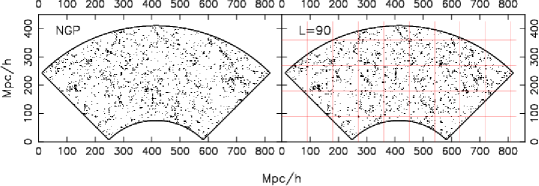
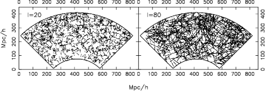
The analysis using “Shuffle” requires us to cut the entire survey area into squares and shuffle them around. The thickness of the resulting subsamples increases with redshift. For our analysis we have considered a smaller region of uniform thickness corresponding to the value at the lowest redshift. For each luminosity bin the area and number density are listed in Table 2. For each bin the galaxy number density varies slightly across the seven strips and the average density along with the $1-\sigma$ variation is shown in Table 2. For all the subsamples, the thickness is much smaller than the other two dimensions and hence it is collapsed along the thickness resulting in a 2D distribution (Figure 1).

We study luminosity dependence of statistically significant length scale of filaments by measuring and comparing it’s value in bin1 and bin2. We label the galaxies in bin1 as Faint and galaxies in bin 2 as Bright.

We also separately study the colour and morphology dependence in bin 2 (Table 1 and Table 2) by dividing the galaxies in this bin into Red/Blue and Early/Late type galaxies. The galaxies in bin 1 are not divided on the basis of their colour or morphology and hence for bin 1 no cut-offs in $u-r$ colour and concentration index $c_{i}$ are listed in Table 2.

Table 1: This shows the $(\lambda,\eta)$ range of the seven non-overlapping strips. For each strip the table shows the number of galaxies in volume limited subsamples bin 1 and bin 2 with absolute magnitude and redshift limits given in Table 2.

Strip number	$\lambda(^{\circ})$	$\eta(^{\circ})$	bin 1	bin 2
1	$-50\leq\lambda\leq 40$	$9\leq\eta\leq 11$	$845$	$1519$
2	$-50\leq\lambda\leq 40$	$11\leq\eta\leq 13$	$743$	$1253$
3	$-60\leq\lambda\leq 30$	$13\leq\eta\leq 15$	$624$	$1153$
4	$-60\leq\lambda\leq 30$	$15\leq\eta\leq 17$	$718$	$1188$
5	$-50\leq\lambda\leq 40$	$21.5\leq\eta\leq 23.5$	$774$	$1381$
6	$-50\leq\lambda\leq 40$	$24\leq\eta\leq 26$	$799$	$1338$
7	$-50\leq\lambda\leq 40$	$26\leq\eta\leq 28$	$781$	$1239$

Table 2: This shows the absolute magnitude and redshift limits for the different volume limited subsamples analyzed. The area and the average galaxy number density with $1-\sigma$ variations from the $7$ strips are also shown. The last two column shows the value of the galaxy colour $(u-r)_{c}$ and the value of the concentration index $c_{i,c}$ used to divide the data into equal numbers of red/blue and elliptical/spiral galaxies respectively. Galaxies in bin 1 are not divided and only galaxies in bin2 are divided to obtain different samples for red/blue and elliptical/spiral galaxies.

bin	Absolute Magnitude range	Redshift range	Area  [ $10^{4}\,h^{-2}\,{\rm Mpc^{2}}$]	Density   [$10^{-2}\,h^{2}{\rm Mpc}^{-2}$]	$(u-r)_{c}$	$c_{i,c}$
bin 1	$-19\geq M_{r}\geq-20$	$0.028014\leq z\leq 0.075635$	$3.35$	$2.25\pm 0.19$	$-$	$-$
bin 2	$-20\geq M_{r}\geq-21$	$0.043657\leq z\leq 0.114635$	$7.47$	$1.73\pm 0.15$	$2.38$	$2.7$

When testing for colour dependence, all the galaxies (Table 1) in the entire area of the bin 2 (Table 2) are classified as either red or blue galaxies. The galaxy $u-r$ colours are known to have a bimodal distribution (Strateva et al., 2001). In our analysis we determine a value $(u-r)_{c}$ for the colour such that it divides galaxies in bin 2 into equal number of red (i.e. $u-r>(u-r)_{c}$) and blue (i.e. $u-r\leq(u-r)_{c}$) galaxies. As a consequence the number density of red and blue galaxies in bin 2 are exactly equal and have a value half that of the density shown in Table 2.

The morphological classification was carried out using the concentration index defined as $c_{i}=r_{90}/r_{50}$ where $r_{90}$ and $r_{50}$ are the radii containing $90\%$ and $50\%$ of the Petrosian flux respectively. This has been found to be one of the best parameter to classify galaxy morphology (Shimasaku et al. 2001). Ellipticals are expected to have a larger concentration indices than spirals. It was found that $c_{i}\simeq 3.33$ for a pure de-Vaucouleurs profile (Blanton et al. 2001) while $c_{i}\simeq 2.3$ for a pure exponential profile (Strateva et al. 2001). In bin 2 we have chosen a cutoff $c_{i,c}$ (Table 2) that partitions the galaxies into two equal halves, one predominantly ellipticals and the other spirals.

2.2 N-body data

We simulate the dark matter distribution using a Particle-Mesh (PM) N-body code. The simulations use $256^{3}$ particles on a $512^{3}$ mesh, and they have a comoving volume $[921.6h^{-1}{\rm Mpc}]^{3}$ . We use $(\Omega_{m0},\Omega_{\Lambda 0},h)=(0.27,0.73,0.71)$ for the cosmological parameters along with a $\Lambda{\rm CDM}\,\,$power spectrum with spectral index $n_{s}=0.96$ and normalization $\sigma_{8}=0.812$ (Komatsu et al. 2008). A “sharp cutoff” biasing, scheme (Cole et al., 1998) was used to extract particles from the N-body simulations. Identifying these particles as galaxies, we have galaxy distributions that are biased relative to the dark matter. The bias parameter $b$ of each simulated galaxy sample was estimated using the ratio

$$b=\sqrt{\frac{\xi_{g}(r)}{\xi(r)}}$$ (1)

where $\xi_{g}(r)$ and $\xi(r)$ are the galaxy and dark matter two-point correlation functions respectively. This ratio is found to be constant at length-scales $r\geq 5h^{-1}{\rm Mpc}$ and we use the average value over $5-40h^{-1}{\rm Mpc}$. We use this method to generate galaxy samples with bias values 1.2, 1.5 and 1.8. We also consider anti bias and galaxy distributions with bias $b=0.8$ were generated by adding randomly distributed particles to the dark matter distribution.

The peculiar velocity effects were included to produce galaxy distributions in redshift space. We have used three independent realisations of the N-body simulations, and for each value of bias we have extracted three different mock data-sets from each simulation. This gives us a total of nine simulated galaxy distribution for each bias values. The simulated galaxy distributions (Figure 1) have the same area, thickness and number density as that of the uniform thickness volume limited subsample constructed out of equatorial strip ($145^{\circ}<\alpha<236^{\circ},-1^{\circ}<\delta<1^{\circ}$) from Northern Galactic Cap (NGP) in Paper I. Each strip extends from $235\,h^{-1}{\rm Mpc}$ to $571\,h^{-1}{\rm Mpc}$ comoving in the radial direction, has uniform thickness of $8.2\,h^{-1}\,{\rm Mpc}$ and contains 1936 galaxies (Table 1 of Paper I). We choose to simulate this strip as we have already established in Paper I that filaments are statistically significant upto length scales $80\,h^{-1}{\rm Mpc}$ and we want to compare this value with that measured from simulations. The simulated data were analyzed in exactly the same way as the actual data.

Earlier studies (Paper II) using N-body simulations show that the filamentarity in the galaxy distribution is sensitive to the area and galaxy number density of the samples. We want to test whether the statistically significant length scale of filaments depends on these factors. We extract regions of identical shape and size similar to the uniform thickness NGP strip in Paper I from dark matter $\Lambda$CDM N-body simulations. We label the mock SDSS NGP strip as density 2 and area 3 in Table 3. Thus effectively the mock SDSS NGP strips, area 3 strips and density 2 strips (Table 3) represent the same galaxy samples. We then prepare different sets of mock galaxy samples which have the same area as SDSS NGP strip but different number densities (density 1, density 3 in Table 3) and other which have the same number densities as SDSS NGP strip but cover different areas (area 1 and area 2 in Table 3). For each sample described in Table 3 we extract three simulated strips from each simulation giving us nine simulated slices. All these simulated slices are analyzed in exactly the same way as the actual data.

Table 3: This shows the redshift limits, area and density for the different mock subsamples analyzed to test the effect of area and density on the statistically significant length scale of filaments.

sample	Redshift range	Area  [ $10^{4}\,h^{-2}\,{\rm Mpc^{2}}$]	Density   [$10^{-2}\,h^{2}{\rm Mpc}^{-2}$]
area 1	$0.01\leq z\leq 0.1$	$6.66$	$9.09$
area 2	$0.05\leq z\leq 0.15$	$13.06$	$9.09$
area 3 (NGP strip)	$0.08\leq z\leq 0.2$	$21.3$	$9.09$
density 1	$0.08\leq z\leq 0.2$	$21.3$	$4.54$
density 2 (NGP strip)	$0.08\leq z\leq 0.2$	$21.3$	$9.09$
density 3	$0.08\leq z\leq 0.2$	$21.3$	$18.17$

Figure 1: This figure exhibits how Shuffle works. The left panel shows the galaxy distribution in a simulated NGP strip from dark matter $\Lambda$CDM N-body simulations and the right panel shows a shuffled realization generated from the same data using $L=90h^{-1}{\rm Mpc}$. A $90h^{-1}{\rm Mpc}\,\times\,90h^{-1}{\rm Mpc}$ grid was placed on the mock NGP data, and square blocks lying fully inside the survey region were randomly shuffled around to generate the data shown in the right panel. This process destroys all coherent structures spanning length-scales larger than $L=90h^{-1}{\rm Mpc}$ in the actual data and filaments larger than this in the shuffled data arise from chance alignments. Among the filaments seen in the right panel, those which run across the block boundaries have formed purely from chance alignments.

Figure 2: This shows the Average Filamentarity as a function of Filling Factor ($FF$) for SDSS galaxies in strip 1 (Table 1) together with the results for the shuffled data for two values of $L$ shown in the figure. Results for different class of galaxies are shown in different panels and indicated in each panel. In all the panels shuffling with $L=10h^{-1}\,{\rm Mpc}$ causes a large drop in the Average Filamentarity showing the statistical significance of the filamentarity at this length-scale. The data is within the $1-\sigma$ error bars of the shuffled realizations for $L=90h^{-1}\,{\rm Mpc}$ (top left panel), $L=70h^{-1}\,{\rm Mpc}$ (top right panel) and $L=80h^{-1}\,{\rm Mpc}$ (bottom left and right panel). The filamentarity is statistically significant up to $L_{MAX}=80,60$ and $70h^{-1}\,{\rm Mpc}$ in these cases where the actual data lies just above the the $1-\sigma$ error bars and are not shown in this figure. For all the larger values of $L$, the data remains within the $1-\sigma$ error bars of the shuffled realizations indicating that the filaments are not statistically significant beyond $L_{MAX}$.

Figure 3: This shows $\chi^{2}/\nu$ at different shuffling lengths for different class of SDSS galaxies as indicated in each panel. The black dotted line indicates $\chi^{2}/\nu=1$.

Figure 4: This shows the results similar to Figure 2 but for a simulated SDSS NGP strip with different bias values as indicated in each panel.

2.3 Segment Cox Process

We use the segment Cox process (Pons-Bordería et al., 1999) to test the reliability of our method in determining the statistically significant length scale of filaments. This is a controlled point process in which the segments of length $l$ are scattered with random positions and orientations within a cube. Points are then randomly distributed on these segments. The length density of the system of segments is $L_{v}=\lambda_{s}\,l$, where $\lambda_{s}$ is the mean number of segments per unit volume. If $\lambda_{l}$ is the mean number of points on a segment per unit length, then the intensity $\lambda$ of the resulting point process is, $\lambda=\lambda_{l}\,L_{v}=\lambda_{l}\,\lambda_{s}\,l$.

For each of the two different segment length ($l=20\,h^{-1}{\rm Mpc}$ and $l=80\,h^{-1}{\rm Mpc}$) we simulate three realizations of segment Cox process inside a cube of side length $L=921.6\,h^{-1}{\rm Mpc}$. We choose the same box size as the N-body simulations used in this paper to enable us to extract regions of identical shape and size similar to the uniform thickness NGP strip used in Paper I. Two different segment lengths are chosen to represent shorter and longer filaments. The different parameters used to simulate the segment Cox process for two different segment lengths are listed in Table 4. We keep the intensity of the resulting point process same in two cases by setting $\lambda_{l}$ fixed and adjusting the value of $\lambda_{s}$ with the value of $l$. Thus we have simulated the segment Cox process for two different values of $l$ and for each values of $l$ the point process is simulated inside three different boxes. We extract three different simulated strips from each of the three boxes giving us a total nine simulated galaxy distribution for each $l$ values. The simulated strips have the same area, thickness and the number density as that of the uniform thickness SDSS NGP strip used in Paper I. The simulated strips are analyzed in exactly the same way as the actual data.

The simulated 2D strips are constructed out of 3D simulations of segment Cox process by slicing and projecting and this fact destroys many segments and shortens many others. We aim to quantify this effect by generating planar (2D) segment Cox process where all the segments lie on the same plane. We simulate the 2D segment Cox process over a planar region which has area and geometry identical to the uniform thickness SDSS NGP strip used in Paper I. The segments of length $l$ are scattered with random positions and orientations within this planar region. Points are then randomly distributed on these segments. The intensity $\lambda$ of the resulting point process is, $\lambda=\lambda_{l}\,\lambda_{s}\,l$ where $\lambda_{s}$ is the mean number of segments per unit area, $\lambda_{l}$ is the mean number of points on a segment per unit length and $l$ is the length of the segments. We simulate 9 such realizations of 2D segment Cox process for each of the two segment lengths ($l=20\,h^{-1}{\rm Mpc}$ and $l=80\,h^{-1}{\rm Mpc}$). The different parameters used to simulate the 2D segment Cox process for two different segment lengths are listed in Table 5. We now randomly extract exactly same number of points as there are in the uniform thickness SDSS NGP strip used in Paper I from each of the 9 realizations of 2D segment Cox process. This gives us a total nine simulated galaxy distribution for each segment lengths (Table 5). The simulated strips have same area, geometry and number density as the SDSS NGP strip. We analyze these simulated strips exactly the same way as the actual data.

Table 4: This shows different parameters used to simulate 3D segment Cox process.

$l$	$\lambda_{s}$	$\lambda_{l}$	$\lambda$
(Segment length)	(Mean no. of segments per unit volume)	(Mean no. of points on a segment per unit length)	(Intensity)
[$h^{-1}\,{\rm Mpc}$]	[$h^{3}\,{\rm Mpc^{-3}}$]	[$h\,{\rm Mpc^{-1}}$]	[$h^{3}\,{\rm Mpc^{-3}}$]
$20$	$0.001278$	$0.8$	$0.020441$
$80$	$0.000319$	$0.8$	$0.020441$

Table 5: This shows different parameters used to simulate 2D segment Cox process.

$l$	$\lambda_{s}$	$\lambda_{l}$	$\lambda$
(Segment length)	(Mean no. of segments per unit area)	(Mean no. of points on a segment per unit length)	(Intensity)
[$h^{-1}\,{\rm Mpc}$]	[$h^{2}\,{\rm Mpc^{-2}}$]	[$h\,{\rm Mpc^{-1}}$]	[$h^{2}\,{\rm Mpc^{-2}}$]
$20$	$0.037612$	$0.8$	$0.601791$
$80$	$0.009403$	$0.8$	$0.601791$

2.4 Method of Analysis

All the strips that we have analyzed are nearly two dimensional. The strips were all collapsed along the thickness (the smallest dimension) to produce 2D galaxy distributions. We use the 2D “Shapefinder” statistic (Bharadwaj et al., 2000) to quantify the average filamentarity of the patterns in the resulting galaxy distribution. A detailed discussion is presented in Paper II , and we present only the salient features here. The reader is referred to Sahni, Sathyaprakash,& Shandarin (1998) for a discussion of Shapefinders in three dimensions.

The galaxy distribution is represented as a set of 1s on a 2-D rectangular grid of spacing $1\,h^{-1}{\rm Mpc}\times 1\,h^{-1}{\rm Mpc}$, empty cells are assigned a value $0$ and filled cells are assigned a value $1$. We identify connected filled cells using the ‘Friends-of-Friend’ (FOF) algorithm. The filamentarity of each cluster is quantified using the Shapefinder ${\cal F}$ defined as

$${\cal F}=\frac{(P^{2}-16S)}{(P-4l)^{2}}$$ (2)

where $P$ and $S$ are respectively the perimeter and the area of the cluster, and $l$ is the grid spacing. The Shapefinder ${\cal F}$ has values $0$ and $1$ for a square and filament respectively, and it assumes intermediate values as a square is deformed to a filament. We use the average filamentarity

$$F_{2}={\sum_{i}{\cal S}_{i}^{2}{\cal F}_{i}\over\sum_{i}{\cal S}_{i}^{2}}\,.$$ (3)

to asses the overall filamentarity of the clusters in the galaxy distribution.

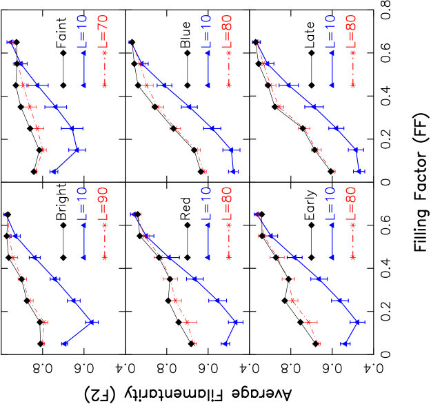
The distribution of 1s corresponding to the galaxies is sparse. Only $\sim 1\%$ of the cells contain galaxies and there are very few filled cells which are interconnected. As a consequence FOF fails to identify the large coherent structures which corresponds to filaments in the galaxy distribution. We overcome this by successively coarse-graining the galaxy distribution. In each iteration of coarse-graining all the empty cells adjacent to a filled cell (i.e. cells at the 4 sides and 4 corners of a filled cell) are assigned a value $1$ . This causes clusters to grow, first because of the growth of individual filled cells, and then by the merger of adjacent clusters as they overlap. Coherent structures extending across progressively larger length-scales are identified in consecutive iterations of coarse-graining. So as not to restrict our analysis to an arbitrarily chosen level of coarse-graining, we study the average filamentarity after each iteration of coarse-graining. The filling factor $FF$ quantifies the fraction of cells that are filled and its value increases from $\sim 0.01$ and approaches $1$ as the coarse-graining proceeds. We study the average filamentarity $F_{2}$ as a function of the filling factor $FF$ (Figure 2) as a quantitative measure of the filamentarity at different levels of coarse-graining. The values of $FF$ corresponding to a particular level of coarse-graining shows a slight variation from strip to strip. In order to combine and compare the results from different strips, for each strip we have interpolated $F_{2}$ to $7$ values of $FF$ at an uniform spacing of $0.1$ over the interval $0.05$ to $0.65$. Coarse-graining beyond $FF\sim 0.65$ washes away the filaments and hence we do not include this range for our analysis.

We use a statistical technique “Shuffle” to determine the largest length-scale at which the filamentarity is statistically significant. A grid with squares blocks of side $L$ is superposed on the original data slice (Figure 1). Blocks of data which lie entirely within the slice are then randomly interchanged, with rotation, repeatedly, to form a new shuffled slice. The shuffling process eliminates coherent features in the original data on scales larger than $L$, keeping clustering at scales below $L$ nearly identical to the original data. All the structures spanning length-scales greater than $L$ that exist in the shuffled slices are the result of chance alignments. At a fixed value of $L$, the average filamentarity in the original sample will be larger than in the shuffled data only if the actual data has more filaments spanning length-scales larger than $L$, than that expected from chance alignments. The largest value of $L$, $L_{\rm MAX}$, for which the average filamentarity of the shuffled slices is less than the average filamentarity of the actual data gives us the largest length-scale at which the filamentarity is statistically significant. Filaments spanning length-scales larger than $L_{\rm MAX}$ arise purely from chance alignments.

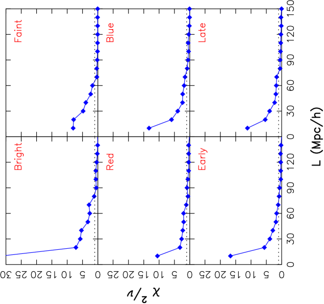
For each value of $L$ we generated $24$ different realization of the shuffled slices. To ensure that the edges of the blocks which are shuffled around do not cut the actual filamentary pattern at exactly the same place in all the realizations of the shuffled data, we randomly shifted the origin of the grid used to define the blocks. The values of FF and $F_{2}$ in the 24 realizations differ from one another and from the actual data at the same stage of coarse-graining. So as to be able to quantitatively compare the shuffled realizations with the actual data, we interpolate the values of $F_{2}$ in the shuffled realization at the same values of FF as interpolated for the actual data. The mean $\bar{F_{2}}[{\rm Shuffled}]$ and the variance $(\Delta F_{2}[{\rm Shuffled}])^{2}$ of the average filamentarity was determined for the shuffled data at each value of FF using the 24 realizations. The difference between the filamentarity of the shuffled data and the actual data was quantified using the reduced $\chi^{2}$ per degree of freedom

$$\frac{\chi^{2}}{\nu}=\frac{1}{N_{p}}\sum_{a=1}^{N_{p}}\frac{(F_{2}[{\rm Actual}]-\bar{F_{2}}[{\rm Shuffled}]))_{a}^{2}}{(\Delta F_{2}[{\rm Shuffled}])_{a}^{2}}$$ (4)

where the sum is over different values of the filling factor FF.

3 Results and Conclusions

We use “Shuffle” to determine the statistically significant length scale of filaments in the seven SDSS strips in magnitude bin 1 and bin 2 (Table 1 and Table 2). We label bin 1 as Faint and bin 2 as Bright. The top two panels of Figure 2 shows the results of “Shuffle” on strip 1 from bin 1 and bin 2 respectively. In top two panels of Figure 2 we see that shuffling the data with $L=10$ causes a large drop in the average filamentarity ($F_{2}$). The average filamentarity increases as the value of $L$ increases and the value of average filamentarity of the unshuffled slice comes within $1-\sigma$ error bars when the data is shuffled with $L=90$ and $L=70$ for Bright and Faint galaxies respectively. Difference between the average filamentarity of shuffled and unshuffled slice is quantified by $\chi^{2}/\nu$ and the top two panels of Figure 3 shows $\chi^{2}/\nu$ as a function of $L$. In top two panels of Figure 3 we see that $\chi^{2}/\nu$ approaches 1 at $L=90$ for Bright and $L=70$ for Faint galaxies. So in strip 1 from bin1 and bin 2 the filaments are statistically significant upto length scales $80\,h^{-1}{\rm Mpc}$ and $60\,h^{-1}{\rm Mpc}$ respectively. The results from the other strips are not shown here. Averaging the results from all the nine strips we find that the filaments are statistically significant upto length scales $84\pm 16\,h^{-1}{\rm Mpc}$ and $71\pm 16\,h^{-1}{\rm Mpc}$ in bin 1 and bin 2 respectively.

The right and left middle panels of Figure 2 shows the results of “Shuffle” for Red and Blue galaxies (Table 2) from strip 1 in bin 2. The right and left middle panels of Figure 2 shows that a large drop in the average filamentarity is observed when the data is shuffled with $L=10$. In both the panels we see that shuffling the data with $L=80$ increase the average filamentarity and brings it back in agreement with the actual data. In two middle panels of Figure 3 we see that in both class of galaxies $\chi^{2}/\nu$ approaches 1 at $L=80$ establishing that for both Red and Blue galaxies the filaments are statistically significant upto length scales $70\,h^{-1}{\rm Mpc}$. Here we have not shown the results from the other strips. Combining results from all the nine strips we find that the filaments are statistically significant upto length scales $77\pm 10\,h^{-1}{\rm Mpc}$ and $71\pm 10\,h^{-1}{\rm Mpc}$ for Red and Blue galaxies respectively.

We show the results of “Shuffle” for the Early and Late type galaxies (Table 2) in the right and left bottom panels of Figure 2. Here also we see that the average filamentarity decreases when the data is shuffled with $L=10$ and it increases and matches with the actual data when the data is shuffled with $L=80$. The $\chi^{2}/\nu$ approaches 1 at $L=80$ for both Early and Late type galaxies as shown in two bottom panels of Figure 3. This establishes that for both Early and Late type galaxies the filaments are statistically significant upto length scales $70\,h^{-1}{\rm Mpc}$ and not beyond. We have shown here only the results for strip 1 in bin 2. Combining the results from all the strips the filaments are found to be statistically significant upto length scales $75\pm 10\,h^{-1}{\rm Mpc}$ and $74\pm 17\,h^{-1}{\rm Mpc}$ for Early and Late type galaxies respectively.

It is to be noted in middle and bottom two panels of Figure 2 that the Red and Early type galaxies have higher degree of filamentarity as compared to Blue and Late type galaxies at smaller values of filling factor. We reported this effect in Pandey & Bharadwaj (2006). It is interesting to note that although the average filamentarity ($F_{2}$) depends on luminosity, colour and morphology of galaxies, the statistically significant length scale of filaments does not depend on these galaxy properties.

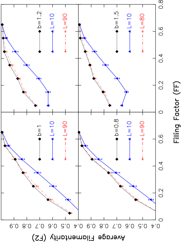
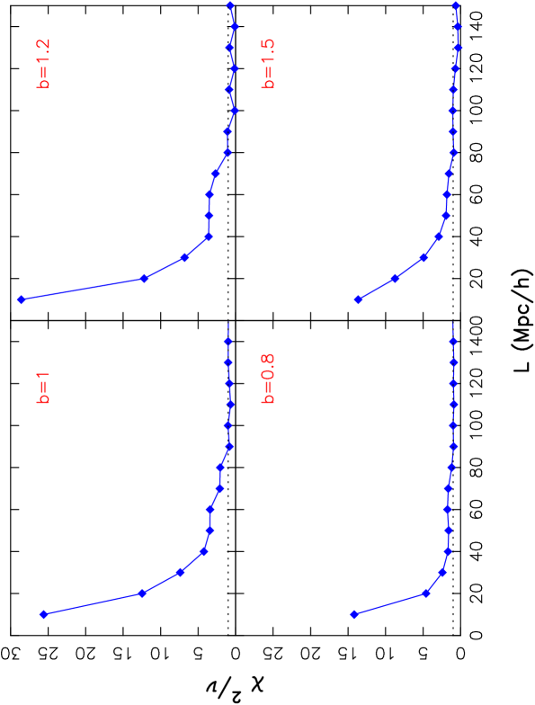
In Figure 4 we show the results of “Shuffle” in simulated SDSS NGP strips with different biases. The top left panel show the result for the dark matter distribution from $\Lambda$CDM N-body simulations. In this case galaxies are assumed to exactly trace the dark matter and the bias parameter $b=1$. We see that shuffling the simulated data with $L=10$ causes a large drop in the average filamentarity of the simulated galaxy distribution. With increasing L the value of average filamentarity of the shuffled slice slowly approaches the values corresponding to the unshuflled data. It is found that at $L=90$ the two are within $1-\sigma$ error bars. The top right panel shows the result for b=1.2. We see a very similar result and the unshuflled and shuffled data agrees well when the data is shuffled with $L=90$. In top left and right panels of Figure 5 we see that $\chi^{2}/\nu$ approaches 1 at $L=90$ for both $b=1$ and $b=1.2$ and hence filaments are statistically significant upto length scales $80\,h^{-1}{\rm Mpc}$ for both cases. The results are shown for one single mock SDSS strip. Averaging the results from all the nine strips it is found that for b=1 and b=1.2 filaments are statistically significant upto length scales $93\pm 16\,h^{-1}{\rm Mpc}$ and $92\pm 15\,h^{-1}{\rm Mpc}$ respectively. The bottom left panel of Figure 4 shows the result of shuffling on simulated SDSS strips for a bias b=0.8. As usual shuffling the data with $L=10$ causes a drop in average filamentarity of the shuffled slice but the drop is smaller as compared to other bias values. As L increases the average filamentarity slowly grows and approaches the values corresponding to the unshuffled data at $L=90$. In the bottom right panel of Figure 4 results are shown for a high bias b=1.5. Shuffling shows similar results for b=1.5 but a relatively large drop is seen when the data is shuffled with $L=10$. With increasing L the average filamentarity grows relatively faster as compared to b=0.8 and finally the average filamentarity in the shuffled data levels up with the unshuffled data when $L=80$ is used for shuffling. In the bottom left and right panels of Figure 5 it is found that $\chi^{2}/\nu$ approaches 1 at $L=90$ and $L=80$ indicating that filaments are statistically significant upto length scales $80\,h^{-1}{\rm Mpc}$ and $70\,h^{-1}{\rm Mpc}$ for b=0.8 and b=1.5 respectively. These are the results shown for a single mock SDSS strip and by combining the results from the other strips we get that the filaments are statistically significant upto length scales $91\pm 13\,h^{-1}{\rm Mpc}$ and $90\pm 15\,h^{-1}{\rm Mpc}$ for $b=0.8$ and $b=1.5$ respectively.

Figure 5: This shows $\chi^{2}/\nu$ at different shuffling lengths for a simulated SDSS NGP strip with different bias values as indicated in each panel. The black dotted line indicates $\chi^{2}/\nu=1$.

Figure 6: This shows the statistically significant length scale of filaments as a function of bias b. The error bars are $1-\sigma$ error bars measured from nine mock galaxy catalogues.

Figure 7: This shows the statistically significant length scale of filaments as a function area of the samples described in Table 3. The error bars are $1-\sigma$ error bars measured from nine mock galaxy catalogues.

Figure 8: This shows the statistically significant length scale of filaments as a function galaxy number density of the samples described in Table 3. The error bars are $1-\sigma$ error bars measured from nine mock galaxy catalogues.

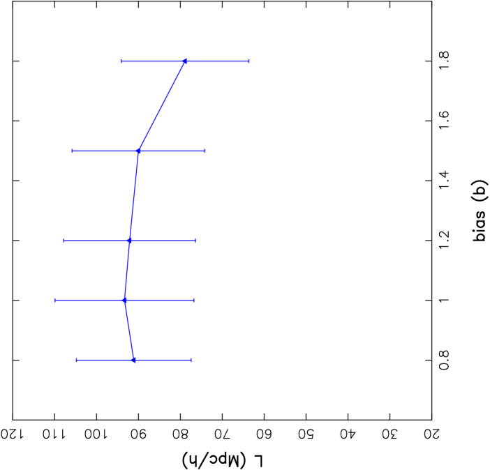
It is to be noted in Figure 4 that as the bias $b$ is increased the average filamentarity ($F_{2}$) increases at smaller $FF$. We reported this effect in Bharadwaj & Pandey (2004). But interestingly the shuffling length at which the avergae filamentarity of the unshuflled and shuffled data agrees does not depend on bias. Figure 6 shows the statistically significant length scale of filaments as a function of bias. This Figure shows that the statistically significant length scale of filaments is nearly independent of bias. The mean value is $~{}90\,h^{-1}{\rm Mpc}$ for the bias values $b=0.8-1.5$. It tends to decrease for a high value of bias $b=1.8$. This could be possibly related to the fact that at very high values of bias we preferentially identify only very high density regions which are mostly related to cluster like structures rather than filaments.

Earlier in Paper I we established that the filaments are statistically significant upto length scales of $80\,h^{-1}{\rm Mpc}$. This measured value lies well within $1-\sigma$ error bars of the measured values for mock galaxy distribution from $\Lambda$CDM N-body simulations. We conclude that the $\Lambda$CDM is consistent with SDSS observations.

The galaxy samples constructed over different magnitude ranges have different area and galaxy number density (Table 2). Earlier analysis in Paper II shows that the average filamentarity of the galaxy distribution depends on the area and galaxy number density of the galaxy samples and filamentarity between different galaxy samples can only be compared when the samples have same area, geometry and number density of galaxies. So it is important to know if the statistically significant length scale of filaments depends on these factors before we can compare it’s measured values among various galaxy samples having different areas and galaxy number densities.

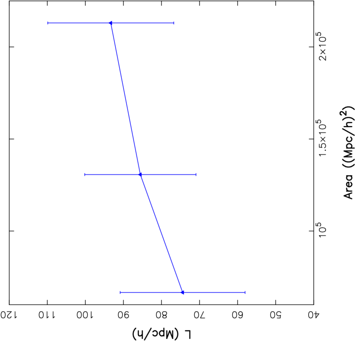
We prepare two different set of mock galaxy samples namely area 1 and area 2 (Table 3) which have the same galaxy number density as the SDSS NGP strip (area 3) but cover different redshift ranges and hence have different areas as listed in Table 3. We extract three mock galaxy samples from each of the $\Lambda$CDM dark matter simulation for each set of galaxy samples area 1 and area 2. We determine the statistically significant length scale of filaments for these galaxy samples. The analysis for the mock SDSS NGP strip which we name as area 3 in Table 3 are already done. We plot the statistically significant length scale of filaments as a function of the area of the galaxy samples in Figure 7. From this figure we see that the samples of smaller area tend to have a smaller length scale of filaments. But this trend is weak and the size of the error bars are quite large. We conclude that the statistically significant length scale of filaments are nearly independent of the area of the samples.

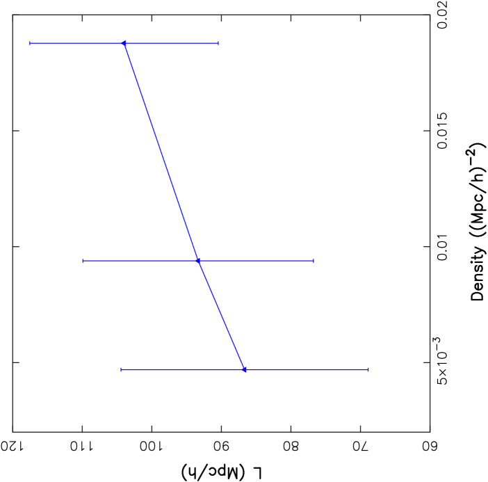
We next prepare two different set of mock galaxy samples namely density 1 and density 3 (Table 3) which have the same area as the SDSS NGP strip (density 2) but have different number densities listed in Table 3. We extract three mock galaxy samples from each of the $\Lambda$CDM dark matter simulation for each set of galaxy samples density 1 and density 3. We determine the statistically significant length scale of filaments for these galaxy samples. The analysis for the mock SDSS NGP strip which we name as density 2 in Table 3 are already done. We plot the statistically significant length scale of filaments as a function of the number density of galaxies of the samples in Figure 8. We see a trend of low density samples to have a smaller length scale of filaments. But the error bars are quite large and the dependence is weak. We conclude that the statistically significant length scale of filaments weakly depends on the number density of galaxies. In a recent work with SDSS LRG samples (Pandey et al., 2009) having much larger area and lower density we find that the statistically significant length scale of filaments does not change much as compared to it’s value measured in SDSS Main galaxy samples. Thus the statistically significant length scale of filaments is a more robust statistics than the average filamentarity. It does not depend on properties (size and number density) of galaxy samples , and physical properties of galaxies. It emerges as a robust measure of the large scale structures. The statistically significant length scale of filaments could be also thought of as an indicator of the scale beyond which the galaxy distribution become homogeneous because it tells us the length scale beyond which no coherent structures exist in the galaxy distribution. Multifractal analysis in SDSS DR1 (Yadav et al., 2005) and recently in SDSS DR6 (Sarkar et al., 2009) show that the galaxy distribution becomes homogeneous at a length scale between $60$ to $70h^{-1}\,{\rm Mpc}$. Yadav et al. (2005) considered the transition to homogeneity in $\Lambda$CDM simulations with different bias $b=1,1.6,2$ and find that irrespective of the bias values the distribution become homogeneous at a length scale between $60$ to $70h^{-1}\,{\rm Mpc}$. These results are consistent with our findings.

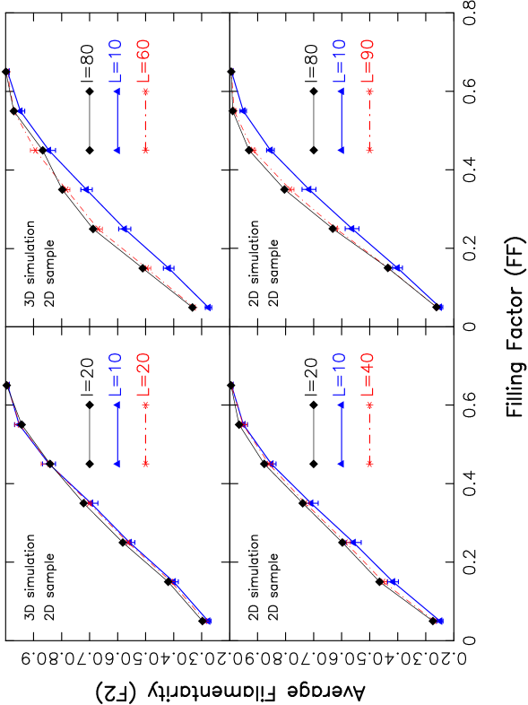
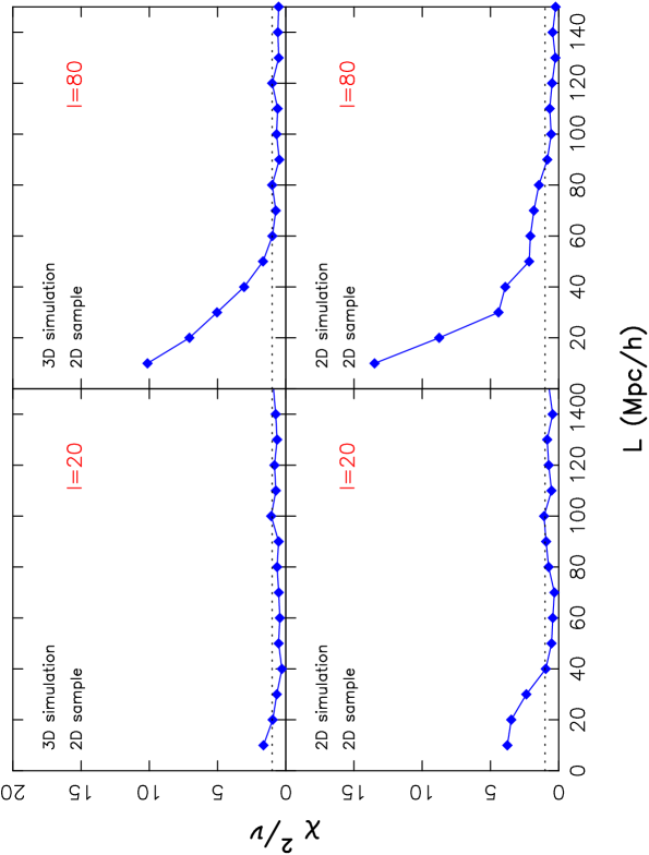
Finally we test the reliability of our method by applying it to different controlled samples (Table 4) of 3D segment Cox process. We use segments of two different length $l=20\,h^{-1}{\rm Mpc}$ and $l=80\,h^{-1}{\rm Mpc}$ for simulating the 3D segment Cox process. Two different sets of 2D mock samples drawn from these 3D simulations (Table 4) are separately analyzed. The results are shown in top two panels of Figure 10 and Figure 11. We see in top left panel of Figure 10 that filamentarity decrease by a very small amount when the mock samples having $l=20\,h^{-1}{\rm Mpc}$ are shuffled with $L=10$ and there are virtually no drop in filamentarity when the data is shuffled with $L=20$. The top right panel of the same figure shows the result of “Shuffle” on cotrolled samples of segment Cox process with segment length $l=80\,h^{-1}{\rm Mpc}$. We see a significant drop in the average filamentarity when the data is shuffled with $L=10$ and the average filamentarity finally saturates to the values corresponding to the unshuffled data when $L=60$ is used for shuffling. The $\chi^{2}/\nu$ as a function of $L$ for these two cases are shown in top two panels of Figure 11. We see that $\chi^{2}/\nu$ approaches 1 at $L=20$ and $L=60$ in these two cases respectively. This indicates that for these 2D mock samples having $l=20\,h^{-1}{\rm Mpc}$ and $l=80\,h^{-1}{\rm Mpc}$, the filaments are found to be statistically significant upto length scales $10\,h^{-1}{\rm Mpc}$ and $50\,h^{-1}{\rm Mpc}$ respectively. Here the results are shown only for a single simulated mock sample. By averaging the results from all the nine simulated mock samples we find that in the above two cases the filaments are statistically significant upto length scales $18\pm 7\,h^{-1}{\rm Mpc}$ and $52\pm 11\,h^{-1}{\rm Mpc}$ respectively. We note that the values of statistically significant length scale of filaments recovered by our method for straight segments simulated here are a little shorter but close to the original values of $l$ used in the simulations. The simulations are carried out in 3D boxes and our mock samples are the 2D projections of nearly two dimensional samples drawn from these boxes. This possibly destroys and shortens a lot of segments and the effects are expected to be more prominent for longer segments as reflected in our results. This effect indicates that also for the 2D real galaxy samples from SDSS which are constructed out of a 3D galaxy distribution, Shuffle possibly underestimates the values of statistically significant length scale of the real 3D filaments.

The effects of slicing and projections can be avoided if we simulate the segment Cox process in 2D as in this case the segments lie on the same plane (Figure 9). We apply Shuffle to a set of mock 2D strips constructed out of simulations of 2D segment Cox process (Table 5). We use two different segment lengths $l=20\,h^{-1}{\rm Mpc}$ and $l=80\,h^{-1}{\rm Mpc}$ to simulate the 2D segment Cox process. We use the same segment lengths as used in the simulations of 3D segment Cox process so as to test the effect of slicing and projection. We show the results in bottom two panels of Figure 10 and Figure 11. Bottom left panel of Figure 10 shows that when the mock samples with $l=20\,h^{-1}{\rm Mpc}$ are shuffled with $L=10$ the average filamentarity of the shuffled data falls below that of the unshuffled data. The average filamentarity of the shuffled data saturates to the unshuffled data when the data is shuffled with $L=40$. The bottom right panel of Figure 10 shows a significant drop in the average filamentarity when the mock samples with $l=80\,h^{-1}{\rm Mpc}$ are shuffled with $L=10$. The average filamentarity of the shuffled data increases slowly with increasing shuffling length and finally saturates to the unshuffled data at shuffling length $L=90$. We see in bottom two panels of Figure 11 the $\chi^{2}/\nu$ as a function of $L$ approaches 1 at $L=40$ and $L=90$ in these two cases respectively. This indicates that for these controlled samples of 2D segment Cox process having $l=20\,h^{-1}{\rm Mpc}$ and $l=80\,h^{-1}{\rm Mpc}$, the filaments are statistically significant upto length scales $30\,h^{-1}{\rm Mpc}$ and $80\,h^{-1}{\rm Mpc}$ respectively. We have shown the results for a single simulated strip in these plots. We combine the results from all the nine simulated strips and find that the filaments are statistically significant upto length scales $25\pm 8\,h^{-1}{\rm Mpc}$ and $82\pm 24\,h^{-1}{\rm Mpc}$ for simulations of 2D segment Cox process with segment length $l=20\,h^{-1}{\rm Mpc}$ and $l=80\,h^{-1}{\rm Mpc}$ respectively. We note that our method can successfully recover better the length of inputted segments when the mock samples are drawn from simulations of 2D segment Cox process where the effects of slicing and projections are absent. There would be another effect due to the boundaries of the samples which again shortens the length of some segments near the boundaries but this effect is not so important in our analysis as the extent of the samples are much larger than the length of the inputted segments. This analysis suggets that the actual length scale of the real 3D filaments can be recovered with Shuffle if the analysis is extended in 3D. We propose to take up this in a future work.

In conclusion we note that although the average filamentarity of the galaxy distribution depends on different galaxy properties, the statistically significant length scale of filaments does not depend on luminosity, colour and morphology of galaxies. We find that the measured values of the statistically significant length scale of filaments in SDSS are consistent with that measured from $\Lambda$CDM simulations. We considered the $\Lambda$CDM model with different values of bias and find that the statistically significant length scale of filaments is nearly independent of bias. Different class of galaxies are differently biased with respect to underlying dark matter distribution and this result is possibly related to the fact that statistically significant length scale of filaments is nearly the same for different class of galaxies. Unlike the average filamentarity, the statistically significant length scale of filaments is nearly independent of the area and galaxy number density of the samples. This establishes the statistically significant length scale of filaments as a robust statistics of galaxy distribution.

Figure 9: This shows a simulation of 2D segment Cox process with two different segment length $l=20\,h^{-1}{\rm Mpc}$ and $l=80\,h^{-1}{\rm Mpc}$ (as indicated in each panel) over a region which has identical geometry to the SDSS NGP equatorial strip. These simulated strips have same values of $l$ and $\lambda_{l}$ listed in Table 5 but different values of $\lambda_{s}$ are chosen so as to lower the density of the segments and make them visibly distinguishable in this plot.

Figure 10: This shows the Average Filamentarity as a function of Filling Factor ($FF$) for a mock SDSS NGP strip constructed out of 3D simulation of segment Cox process (Table 4) and 2D simulation of segment Cox process (Table 5) together with the results for the shuffled data for two values of $L$ shown in the figure. The 2D simulations of segment Cox process contain all the segments in the same plane and there are no effects because of the slicing process or the projections which arises when samples are constructed out of 3D simulations of segment Cox process. We see in this plot that “Shuffle” is able to recover the length of the longer segments more efficiently when samples are constructed out of 2D simulations instead of 3D simulations of segment Cox process.

Figure 11: This shows $\chi^{2}/\nu$ at different shuffling lengths ($L$) for a mock SDSS NGP strip constructed out of 3D segment Cox process and 2D segment Cox process simulated with two different segment length $l=20\,h^{-1}{\rm Mpc}$ and $l=80\,h^{-1}{\rm Mpc}$. The black dotted line indicates $\chi^{2}/\nu=1$.

4 Acknowledgment

BP acknowledges Somnath Bharadwaj for useful discussions and suggestions. Thanks are due to an anonymous referee, whose comments and suggestions led to significant improvement of the paper. The SDSS DR6 data was downloaded from the SDSS skyserver http://cas.sdss.org/dr6/en/ .

Funding for the creation and distribution of the SDSS Archive has been provided by the Alfred P. Sloan Foundation, the Participating Institutions, the National Aeronautics and Space Administration, the National Science Foundation, the U.S. Department of Energy, the Japanese Monbukagakusho, and the Max Planck Society. The SDSS Web site is http://www.sdss.org/.

The SDSS is managed by the Astrophysical Research Consortium (ARC) for the Participating Institutions. The Participating Institutions are The University of Chicago, Fermilab, the Institute for Advanced Study, the Japan Participation Group, The Johns Hopkins University, the Korean Scientist Group, Los Alamos National Laboratory, the Max-Planck-Institute for Astronomy (MPIA), the Max-Planck-Institute for Astrophysics (MPA), New Mexico State University, University of Pittsburgh, Princeton University, the United States Naval Observatory, and the University of Washington.

References

- Adelman-McCarthy et al. (2008) Adelman-McCarthy, J. K., et al. 2008, ApJS, 175, 297
- Aragón-Calvo et al. (2007) Aragón-Calvo, M. A., van de Weygaert, R., Jones, B. J. T., & van der Hulst, J. M. 2007, ApJL, 655, L5
- Barrow et al. (1985) Barrow, J. D., Bhavsar, S. P., & Sonoda, D. H. 1985, MNRAS, 216, 17
- Basilakos, Plionis, & Rowan-Robinson (2001) Basilakos, S., Plionis, M., & Rowan-Robinson, M. 2001, MNRAS, 323, 47
- Bharadwaj et al. (2000) Bharadwaj, S., Sahni, V., Sathyaprakash, B. S., Shandarin, S. F., & Yess, C. 2000, ApJ, 528, 21
- Bharadwaj, Bhavsar & Sheth (2004) Bharadwaj, S., Bhavsar, S. P., & Sheth, J. V. 2004, ApJ, 606, 25
- Bharadwaj & Pandey (2004) Bharadwaj, S., Pandey, B. 2004, ApJ, 615, 1
- Bhavsar & Ling (1988) Bhavsar, S. P. & Ling, E. N. 1988, ApJL, 331, L63
- Blanton et al. (2001) Blanton, M. R., et al. 2001, AJ, 121, 2358
- Cole et al. (1998) Cole, S., Hatton, S., Weinberg, D. H., & Frenk, C. S. 1998, MNRAS, 300, 945
- Colberg et al. (2005) Colberg, J. M., Krughoff, K. S., & Connolly, A. J. 2005, MNRAS, 359, 272
- Colles et al. (2001) Colles, M. et al.(for 2dFGRS team) 2001,MNRAS,328,1039
- Doroshkevich et al. (2004) Doroshkevich, A., Tucker, D. L., Allam, S.,& Way, M. J. 2004, A&A, 418,7
- Einasto et al. (1980) Einasto, J., Joeveer, M., & Saar, E. 1980, MNRAS, 193, 353
- Einasto et al. (1984) Einasto, J., Klypin, A. A., Saar, E., & Shandarin, S. F. 1984, MNRAS, 206, 529
- Efstathiou et al. (2001) Efstathiou, G. , et al. 2002, MNRAS, 330, L29
- Fukugita et al. (1996) Fukugita, M., Ichikawa, T., Gunn, J. E., Doi, M., Shimasaku, K., & Schneider, D. P. 1996, AJ, 111, 1748
- Geller & Huchra (1989) Geller, M.J. & Huchra, J.P.1989, Science, 246, 897
- Gott, Dickinson, & Melott (1986) Gott, J. R., Dickinson, M., & Melott, A. L. 1986, ApJ, 306, 341
- Gunn et al. (2006) Gunn, J. E., et al. 2006, AJ, 131, 2332
- Icke & van de Weygaert (1987) Icke, V., & van de Weygaert, R. 1987, A&A, 184, 16
- Joeveer et al. (1978) Joeveer, M., Einasto, J., & Tago, E. 1978, MNRAS, 185, 357
- Kaiser (1984) Kaiser, N. 1984, ApJL, 284, L9
- Komatsu et al. (2008) Komatsu, E., et al. 2009, ApJS, 180, 330
- Mecke et al. (1994) Mecke, K. R., Buchert, T., & Wagner, H. 1994, A&A, 288, 697
- Mo & White (1996) Mo, H.J.& White, S.D.M. 1996, MNRAS, 282, 347
- Müller et al. (2000) Müller, V., Arbabi-Bidgoli, S., Einasto, J., & Tucker, D. 2000, MNRAS, 318, 280
- Pandey & Bharadwaj (2005) Pandey, B. & Bharadwaj, S. 2005, MNRAS, 357, 1068
- Pandey & Bharadwaj (2006) Pandey, B. & Bharadwaj, S. 2006, MNRAS, 372, 827
- Pandey & Bharadwaj (2007) Pandey, B., & Bharadwaj, S. 2007, MNRAS, 377, L15
- Pandey & Bharadwaj (2008) Pandey, B., & Bharadwaj, S. 2008, MNRAS, 387, 767
- Pandey et al. (2009) Pandey, B., Kulkarni, G., Bharadwaj, S. & Souradeep, T. 2009, in preparation
- Percival et al. (2001) Percival, W. J., et al. 2001, MNRAS, 327, 1297
- Pimbblet & Drinkwater (2004) Pimbblet, K. A., & Drinkwater, M. J. 2004, MNRAS, 347, 137
- Pimbblet, Drinkwater & Hawkrigg (2004) Pimbblet, K. A., Drinkwater, M. J., & Hawkrigg, M. C. 2004, MNRAS, 354, L61
- Pimbblet (2005) Pimbblet, K. A. 2005, Publications of the Astronomical Society of Australia, 22, 136
- Pons-Bordería et al. (1999) Pons-Bordería, M.-J., Martínez, V. J., Stoyan, D., Stoyan, H., & Saar, E. 1999, ApJ, 523, 480
- Sahni, Sathyaprakash,& Shandarin (1998) Sahni, V., Sathyaprakash, B. S., & Shandarin, S. F. 1998, ApJL, 495, L5
- Sarkar & Bharadwaj (2009) Sarkar, P., & Bharadwaj, S. 2009, MNRAS, 394, L66
- Sarkar et al. (2009) Sarkar, P., Yadav, J., Pandey, B., & Bharadwaj, S. 2009, MNRAS, L306
- Schmalzing & Buchert (1997) Schmalzing, J., & Buchert, T. 1997, ApJL, 482, L1
- Shandarin & Zeldovich (1983) Shandarin, S. F. & Zeldovich, I. B. 1983, Comments on Astrophysics, 10, 33
- Shandarin & Yess (1998) Shandarin, S. F. & Yess, C. 1998, ApJ, 505, 12
- Shectman et al. (1996) Shectman, S. A.,Landy, S. D., Oemler, A., Tucker, D. L., Lin, H., Kirshner, R. P., & Schechter, P. L. 1996, ApJ, 470, 172
- Shimasaku et al. (2001) Shimasaku, K., et al. 2001, AJ, 122, 1238
- Spergel et al. (2003) Spergel, D. N. et al. 2003, ApJ, 148, 175
- Spergel et al. (2007) Spergel, D. N., et al. 2007, ApJS, 170, 377
- Stoica et al. (2005) Stoica, R. S., Martínez, V. J., Mateu, J., & Saar, E. 2005, A&A, 434, 423
- Stoica et al. (2007) Stoica, R. S., Martínez, V. J., & Saar, E. 2007, Journal of the Royal Statistical Society: Series C (Applied Statistics) 56 (4), 459-477, 56, 1
- Stoughton et al. (2002) Stoughton, C., et al. 2002, AJ, 123, 485
- Strateva et al. (2001) Strateva, I., et al. 2001, AJ, 122, 1861
- Strauss et al. (2002) Strauss, M. A., et al. 2002, AJ, 124, 1810
- Sousbie et al. (2008) Sousbie, T., Pichon, C., Colombi, S., Novikov, D., & Pogosyan, D. 2008, MNRAS, 383, 1655
- Tegmark et al. (2004) Tegmark, M., et al. 2004 , PRD, 69, 103501
- van de Weygaert & Icke (1989) van de Weygaert, R., & Icke, V. 1989, A&A, 213, 1
- Yadav et al. (2005) Yadav, J., Bharadwaj, S., Pandey, B., & Seshadri, T. R. 2005, MNRAS, 364, 601
- York et al. (2000) York, D. G., et al. 2000, AJ, 120, 1579
- Zel’dovich , Einasto & Shandarin (1982) Zel’dovich, I. B., Einasto, J., & Shandarin, S. F. 1982, Nature, 300, 407