Pressure Support vs. Thermal Broadening in the Lyman-$\alpha$ Forest I:
Effects of the Equation of State on Longitudinal Structure

Abstract

In the low density intergalactic medium (IGM) that gives rise to the Lyman-$\alpha$ forest, gas temperature and density are tightly correlated. The velocity scale of thermal broadening and the Hubble flow across the gas Jeans scale are of similar magnitude ($H\lambda_{J}\sim\sigma_{\rm th}$). To separate the effects of gas pressure support and thermal broadening on the Ly$\alpha$ forest, we compare spectra extracted from two smoothed particle hydrodynamics (SPH) simulations evolved with different photoionization heating rates (and thus different Jeans scales) and from the pressureless dark matter distribution, imposing different temperature-density relations on the evolved particle distributions. The dark matter spectra are similar but not identical to those created from the full gas distributions, showing that thermal broadening sets the longitudinal (line-of-sight) scale of the Ly$\alpha$ forest. The turnover scales in the flux power spectrum and flux autocorrelation function are determined mainly by thermal broadening rather than pressure. However, the insensitivity to pressure arises partly from a cancellation effect with a sloped temperature-density relation ($T\propto\rho^{0.6}$ in our simulations): the high density peaks in the colder, lower pressure simulation are less smoothed by pressure support than in the hotter simulation, and it is this higher density gas that experiences the strongest thermal broadening. Changes in thermal broadening and pressure support have comparably important effects on the flux probability distribution (PDF), which responds directly to the gas overdensity distribution rather than the scale on which it is smooth. Tests on a lower resolution simulation ($2\times 144^{3}$ vs. $2\times 288^{3}$ particles in a $12.5h^{-1}\,{\rm Mpc}$ comoving box) show that our statistical results are converged even at this lower resolution. While thermal broadening generally dominates the longitudinal structure in the Ly$\alpha$ forest, we show in Paper II that pressure support determines the transverse coherence of the forest observed towards close quasar pairs.

1 Introduction

The Lyman-$\alpha$ forest, caused by Ly$\alpha$ absorption of neutral hydrogen atoms along the line of sight to some distant source (usually a quasar), was originally described in terms of discrete intervening gas “clouds” (Lynds, 1971; Sargent et al., 1980), analogous to clouds in the Galactic interstellar medium. In this picture, the velocity widths of the observed absorption structures were primarily a consequence of thermal motions of the absorbing atoms. In the mid-1990s, three-dimensional hydrodynamic simulations of cold dark matter (CDM) cosmological models achieved remarkable success in reproducing the observed properties of the Ly$\alpha$ forest (Cen et al., 1994; Zhang et al., 1995; Hernquist et al., 1996; Miralda-Escudé et al., 1996; Theuns et al., 1998). In these simulations, most of the absorbing gas is at low density ($\rho/\bar{\rho}\sim 0.1$–10) and naturally described as a continuously fluctuating medium rather than a series of discrete structures (Hernquist et al., 1996; Bi & Davidsen, 1997; Rauch et al., 1997; Croft et al., 1997, 1998). The velocity width of individual features is set largely by the Hubble flow across them, reflecting the physical extent of the absorbing gas along the line of sight (Hernquist et al., 1996; Weinberg et al., 1997). The temperature of the intergalactic medium (IGM), therefore, affects the structure of the Ly$\alpha$ forest in two ways: by smoothing absorption along the line of sight through the thermal motions of atoms, and by smoothing the physical distribution of the gas in three dimensions through pressure support. In this study, we use two smoothed particle hydrodynamics (SPH) simulations with different photoionization heating rates—and thus different IGM temperatures and amounts of gas pressure support—to disentangle the relative effects of pressure support and thermal broadening in the Ly$\alpha$ forest.

Both hydrodynamical simulations (Katz et al., 1996; Miralda-Escudé et al., 1996; Theuns et al., 1998) and analytic arguments (Hui & Gnedin, 1997) suggest that low-density intergalactic gas should have a power-law temperature-density relation, i.e., $T=T_{0}(1+\delta)^{\alpha}$, where $1+\delta\equiv\rho/\bar{\rho}$ is the local gas overdensity. Reasonable assumptions for heating and cooling rates yield $T_{0}\sim 10^{4}$ K and $\alpha\sim 0.6$ (Hui & Gnedin, 1997; Theuns et al., 1998). Observations, however, imply that the normalization $T_{0}$ could be nearly twice as high, and the slope could be much shallower or even inverted (Schaye et al., 1999; Ricotti et al., 2000; McDonald et al., 2001; Bolton et al., 2008). Regardless of the parameter values, because the optical depth to Ly$\alpha$ absorption is related to both the temperature and the density by a power law, the existence of the temperature-density relation (also called the “equation of state”) implies a tight relation between the observed Ly$\alpha$ absorption and the IGM gas density. Since the universe has $\sim 5$ times as much mass in dark matter as in baryons, we can expect in general for intergalactic gas to trace the underlying dark matter on scales above the gas Jeans length (Schaye, 2001). The Ly$\alpha$ forest therefore provides a powerful tool for tracing the dark matter power spectrum in the quasi-linear regime—modulo the effects of peculiar velocities, thermal broadening, and gas pressure (Croft et al., 1998, 1999, 2002; McDonald et al., 2000, 2006; Viel et al., 2004; Viel & Haehnelt, 2006).

Pressure should be important on scales at or below the Jeans length,

$$\lambda_{J}=c_{s}\sqrt{\frac{\pi}{G\rho}}=\sigma_{\rm th}\sqrt{\frac{5\pi}{3G\rho}},$$ (1)

where $c_{s}=\sqrt{[5kT]/[3m]}=\sigma_{\rm th}\sqrt{5/3}$ is the speed of sound in an ideal gas expressed as a multiple of the 1-D thermal velocity $\sigma_{\rm th}$ (Miralda-Escudé et al., 1996; Schaye, 2001; Desjacques & Nusser, 2005). Here $m$ is the average mass of the gas particle; in an ionized primordial mixture of hydrogen and helium, $m=0.59m_{p}$, where $m_{p}$ is the proton mass. The density $\rho$ is the density of the gravitating medium, which is dominated by dark matter, so we take $\rho=\Omega_{m,0}\rho_{c,0}(1+z)^{3}(1+\delta)$. In comoving coordinates,

$$\lambda_{J,{\rm comv}} = (1+z)\sigma_{\rm th}H_{0}^{-1}\sqrt{\frac{5\pi}{3}}\left[\frac{3}{8\pi}\Omega_{m,0}(1+z)^{3}(1+\delta)\right]^{-1/2}$$

$$= 782\,h^{-1}\,\mbox{kpc}$$

$$\times \left(\frac{\sigma_{\rm th}}{11.8\,\rm{km}\,\rm{s}^{-1}}\right)\left[\left(\frac{\Omega_{m,0}(1+\delta)}{0.25\times(1+0)}\right)\left(\frac{1+z}{1+3}\right)\right]^{-1/2},$$

where we have normalized the thermal broadening velocity $\sigma_{\rm th}$ to correspond to a fiducial temperature of $10^{4}$ K. By defining a “Jeans velocity” as $v_{J}\equiv H\lambda_{J}$ we can find the relative importance of the Jeans scale and $\sigma_{\rm th}$,

$$\frac{v_{J}}{\sigma_{\rm th}} = \frac{2\pi\sqrt{10}}{3}(1+\delta)^{-1/2}\left[\frac{\Omega_{m,0}(1+z)^{3}+\Omega_{\Lambda}}{\Omega_{m,0}(1+z)^{3}}\right]^{1/2}$$

$$\approx 6.62(1+\delta)^{-1/2},$$

which is essentially redshift-independent for the redshifts relevant to the Ly$\alpha$ forest. The Jeans length of equation (1) divides stable from unstable modes in a static, homogeneous, self-gravitating medium. The IGM is expanding, inhomogeneous, non–self-gravitating (because dark matter dominates), and evolving in density and temperature on the same timescale that fluctuations grow. Even for linear perturbations in a baryonic universe, the “filtering scale” below which fluctuations growth is suppressed depends on the thermal history of the gas rather than the instantaneous temperature-density relation (Gnedin & Hui, 1998). We therefore expect equation (1) to describe the scale of gas pressure support only at an order-of-magnitude level. Equation (1) shows that Jeans velocities and thermal velocities should be comparable at the overdensities of typical Ly$\alpha$ forest features, but the calculation is not definitive enough to show whether one will dominate in practice.

Hence, to predict the statistical properties of the Ly$\alpha$ forest in a given cosmological model, one must calculate the predicted gas distribution. The most reliable way to do this uses full $N$-body plus hydrodynamic simulations, which include the gravity of dark matter and gas and the additional effects of pressure, adiabatic heating and cooling, heating by photoionization and shocks, and radiative cooling. However, large volume hydrodynamic simulations with the necessary resolution are computationally intensive. Weinberg et al. (1997) and Croft et al. (1998) show that one can achieve reasonable accuracy in the Ly$\alpha$ forest regime from pure dark matter simulations, applying the temperature-density relation to the evolved dark matter distribution to compute spectra. Indeed, the log-normal model (Bi & Davidsen, 1997), in which the dark matter distribution is computed from the linear density field by an exponential transformation (Coles & Jones, 1991), provides a qualitatively accurate physical model of the Ly$\alpha$ forest, sufficient for creating artificial spectra with reasonable statistical properties.

A fast way to include the effects of gas pressure in an approximate way is the hydrodynamic particle-mesh (HPM) method (Gnedin & Hui, 1998; Ricotti et al., 2000; Meiksin & White, 2001). HPM assumes that all the gas follows the power-law IGM equation of state, and it uses a modification of the standard (fast) particle-mesh $N$-body method to compute the sum of gravitational forces and pressure gradient forces given this equation of state. In a detailed comparison of fully hydrodynamic SPH simulations and the approximated HPM simulations, both evolved using Gadget-2, Viel et al. (2004) found that while the HPM approach does converge to the SPH results, for some Ly$\alpha$ forest properties, such as the flux probability distribution or small-scale power spectrum, it can differ from the SPH calculation by as much as 50% at $z\sim 2$. A simpler alternative to HPM is to use a pure $N$-body simulation but smooth the evolved dark matter distribution on the Jeans scale before extracting Ly$\alpha$ forest spectra (Zaldarriaga et al., 2001; Desjacques & Nusser, 2005). Because the Jeans smoothing is three-dimensional, it is not degenerate with line-of-sight thermal broadening. Zaldarriaga et al. (2001) found that, even though the thermal broadening dominates the pressure correction, the value of the Jeans length becomes a large source of uncertainty in cosmological inferences from the Ly$\alpha$ forest if one tries to estimate it from the data rather than predict it from theory. Because the Jeans length is expected to vary with the gas temperature and density, a Zel’dovich-like scheme can be used when smoothing the dark matter distribution in order to model these effects (Viel et al., 2002). Though we do not carry out a comprehensive comparison of these methods here, we do investigate the impact of pressure in detail, as well as compare full SPH simulations to results derived from the dark matter distribution alone.

The primary purpose of this paper and its companion (Peeples et al. 2009, hereafter Paper II) is to disentangle the roles of pressure support and thermal broadening in the Ly$\alpha$ forest by studying two SPH simulations with different thermal histories and temperature-density relations. In addition to examining the physics of the Ly$\alpha$ forest, this study is motivated by observational evidence (discussed in § 3.1) that the temperature of the IGM at $z\sim 2$–4 is higher than expected from simple photoionization models by a factor of 1.5–2. This evidence comes from analyses of data along single lines of sight. Because the higher pressure associated with hotter gas would smooth the IGM in three dimensions, using closely paired lines of sight to probe this coherence scale has been proposed as an alternative route for inferring the temperature-density relation (J. Hennawi, private communication, 2007). However, before we can understand the relative roles of temperature and pressure on the transverse structure of the Lyman-$\alpha$ forest, we must first understand their longitudinal effects along independent sightlines, which is the goal of this paper. While here we find that thermal broadening dominates pressure support in setting the level of longitudinal structure in the Ly$\alpha$ forest, in Paper II we show that the gas Jeans length dominates the level of coherence transverse to the line of sight.

This paper is organized as follows. In § 2, we describe the SPH simulations we have evolved to investigate these effects. In § 3, we describe the physics of the Ly$\alpha$ forest in these simulations and examine the impact of the thermal history on observable spectra; this section also serves to review the physical understanding of the high-redshift Ly$\alpha$ forest that has emerged from simulations and associated analytic work since the mid-1990s. We then study these effects on several typical statistical measures for learning about the IGM from the Ly$\alpha$ forest in § 4, with our conclusions in § 5.

2 Simulations

We analyze two SPH simulations with identical initial conditions, one with a fiducial photoionization heating rate and one with a heating rate from photoionization that is four times higher than the fiducial; hereafter, we refer to these simulations as the “fiducial” and “H4” simulations, respectively. In the terminology of Katz et al. (1996), we compute the photoionization rates $\Gamma$ and photoionization heating rates $\epsilon$ for the fiducial simulation assuming the Haardt & Madau (2001) quasar $+$ galaxy photoionizing background, and for the H4 simulation we increase $\epsilon_{\rm H\,I}$, $\epsilon_{\rm He\,I}$, and $\epsilon_{\rm He\,II}$ by a factor of four. In principle, these heating rates could arise from a much harder UV background spectrum that yields more residual energy per photo-electron. However, we do not propose any specific model for these heating rates—they are a computationally simple way to obtain IGM temperatures that are higher than those in the fiducial model and closer to those estimated from observations (see § 3.1 for further discussion).

We evolve these SPH simulations using the parallel Gadget-2 code (Springel, 2005) to trace the evolution of $288^{3}$ dark matter and $288^{3}$ gas particles in a $12.5\,h^{-1}$ Mpc comoving cubic volume from $z=15$ to $z=2$. We also evolved another simulation using the fiducial heating rates and the same initial conditions but only $2\times 144^{3}$ particles to serve as a test for resolution convergence. We adopt a standard $\Lambda$CDM cosmological model with the parameters $(\Omega_{M},\Omega_{\Lambda},\Omega_{b},h,\sigma_{8},n_{s})=(0.25,0.75,0.044,0.7,0.8,0.95)$, all of which are in good agreement with the Wilkinson Microwave Anisotropy Probe (WMAP) five-year results (Hinshaw et al., 2009); our choice of $\sigma_{8}=0.8$, however, is somewhat lower than what is typically considered for Ly$\alpha$ studies. These parameters give a mass per SPH particle of $1.426\times 10^{6}\mbox{M}_{\odot}$, which is much less than the typical Jeans mass of $M_{J}\equiv\rho\lambda_{J}^{3}\sim 7\times 10^{9}\mbox{M}_{\odot}$. The spline gravitational force softening has an equivalent Plummer length of $0.875\,h^{-1}$ kpc comoving ($\sim 1/50$ of the initial particle grid spacing). The SPH smoothing lengths are chosen to enclose $33\pm 2$ neighbors within the smoothing kernel. The simulation incorporates standard heating and atomic cooling processes and the standard Gadget-2 treatment of star formation and metal enrichment. These simulations do not incorporate galactic winds, but these should have very little effect on the Ly$\alpha$ forest (Kollmeier et al., 2006; Bertone & White, 2006; Marble et al., 2008).

We extract spectra from the SPH gas distribution using TIPSY, as described by Hernquist et al. (1996). Following common practice, we rescale the intensity of the UV background so that the mean flux decrement of the extracted spectra matches observations (Table 1), as the mean decrement itself is much better known than the background intensity (see discussions by, e.g., Croft et al. 2002; Marble et al. 2008). Our extracted spectra have 1250 pixels across the $12.5h^{-1}$ Mpc volume, making the pixel size $\approx 1$ km s^-1, which is well below the smoothing scale imposed by thermal broadening.

3 Physics of the Lyman-$\alpha$ forest

3.1 The Temperature-Density Relation

In the absence of shock heating, the evolution of the temperature of the IGM is described by

$$\frac{\mbox{d}T}{\mbox{d}z}=\frac{2T}{1+z}+\left[\frac{2T}{3(1+\delta)}\right]\frac{\mbox{d}\delta}{\mbox{d}z}-\left[\frac{T}{m}\right]\frac{\mbox{d}m}{\mbox{d}z}+\frac{2}{3k_{\mbox{\tiny$B$}}n_{b}}\frac{\mbox{d}Q}{\mbox{d}z},$$ (4)

as shown in detail by Hui & Gnedin (1997). Here, $\mbox{d}\delta/\mbox{d}z$ and $H(z)$ depend on the cosmology, the overdensity $1+\delta\equiv(\rho_{\rm gas}/\bar{\rho}_{\rm b})$, $m$ is the mean particle mass, and $\mbox{d}Q/\mbox{d}z$ is the net power per unit volume owing to the ambient radiation field. The first two terms in equation (4) describe heating and cooling owing to adiabatic processes. After reionization, the change in temperature owing to the change in the ionization fraction (the third term in equation [4]) is effectively zero at all redshifts and relevant densities.

Hydrogen reionization produces one energetic photoelectron per hydrogen atom, and it is expected to heat the IGM to a temperature $T\sim 2$–$5\times 10^{4}$ K, depending on the spectral shape of the ionizing sources and radiative transfer effects (Miralda-Escudé & Rees, 1994). Thereafter, adiabatic cooling reduces the overall temperature, but denser regions remain hotter because they have higher neutral fractions and thus higher photoionization heating rates. At a given redshift, the simulated temperature-density ($T$-$\rho$) relation of the photoionized medium can be well approximated by a powerlaw,

$$T(z)=T_{0}(z)(1+\delta)^{\alpha(z)}.$$ (5)

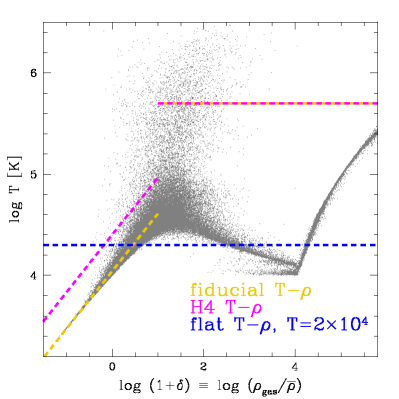
The slope $\alpha(z)$ approaches $0.6$ well after reionization. Evolution with the Haardt & Madau (2001) UV background spectrum and $\Omega_{b}h^{2}\approx 0.022$ yields $T_{0}\approx 10^{4}$ K at $z=2$–4, for reionization at $z\gtrsim 7$ (e.g., Hui & Gnedin 1997; Theuns et al. 1998; Davé et al. 1999; Table 1). Figure 1 shows the distribution of SPH particles for our fiducial simulation in the temperature-overdensity plane at $z=3$. At low overdensities ($1+\delta\lesssim 10$), most of the gas falls along a tight locus, as expected from the above discussion. At higher densities ($1+\delta\gtrsim 100$), the gas has begun to cool to form galaxies. The higher temperature gas has been shock heated. (The apparent increase in temperature at $1+\delta\sim 10^{4}$ owes to the way Gadget-2 treats the multiphase interstellar medium.) For many of our subsequent analyses, we will isolate physical effects by imposing one of the three $T$-$\rho$ relations, denoted by dashed lines in Figure 1. Specifically, we assign each gas (or dark matter) particle the temperature implied by its overdensity and a given $T$-$\rho$ relation before extracting spectra. The yellow line is an eyeball fit to the $T$-$\rho$ relation in the fiducial simulation, while the pink line is the corresponding fit to the H4 relation; the H4 $T$-$\rho$ normalization is $\sim 2.3$ times higher than the fiducial normalization. In both of these cases we set gas with $1+\delta>10$ to a “shocked” temperature of $T=5\times 10^{5}$ K, so that this high density gas will be entirely ionized and thus not contribute to the Ly$\alpha$ forest. The mass- and volume-fraction of gas in these high density regions is relatively tiny; for all of the statistics presented here, the fiducial and H4 gas distributions using the imposed fiducial and H4 $T$-$\rho$ relations, respectively, yield nearly identical results to those obtained using the actual temperatures calculated by Gadget-2. Parameters for these fits are listed in Table 1. For some comparisons, we impose a flat $T$-$\rho$ relation, with all particles set to $T=2\times 10^{4}$ K, as shown by the blue dashed line.

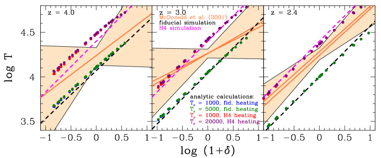
Although most Ly$\alpha$ forest features are broadened by Hubble flow, the narrowest features arise at velocity caustics and have widths set by thermal broadening. Analyses of observed line width distributions imply $T_{0}\approx 1.5$–$2\times 10^{4}$ K at $2\leq z\leq 4$ (Gnedin & Hui 1998; Ricotti et al. 2000; Schaye et al. 2000; McDonald et al. 2001; we adopt McDonald et al.’s constraints in Table 1 and Figure 2). This is significantly hotter than the value $T_{0}\approx 10^{4}$ K expected for a Haardt & Madau (2001) ionizing background. Theuns et al. (2000) and Zaldarriaga et al. (2001) find a similar result by fitting the small-scale cutoff of the one-dimensional flux power spectrum. More recently, Bolton et al. (2008) have fit the flux probability distribution function (PDF) in high-resolution spectra inferring a similar, high $T_{0}$ and a shallow, possibly inverted ($\alpha<0$) slope. Lidz et al. (2009) find $T_{0}\approx 2\times 10^{4}$ K over the redshift range $z=2$–4, using a wavelet analysis of 40 high-resolution spectra. In all cases, the observations are interpreted by comparing them to a suite of cosmological simulations, which incorporate many parameters in addition to the $T$-$\rho$ relation itself.

Figure 1: Distribution of 1% of the gas particles for the fiducial simulation in the temperature-density plane at $z=3$. In subsequent analyses, we use either the simulation temperatures themselves or one of the three plotted $T$-$\rho$ relations (dashed lines).

According to equation (4), there are two basic ways to increase the gas temperature: either have hotter “initial conditions,” or a higher heating rate $\mbox{d}Q/\mbox{d}z$. Even with the highest plausible reionization temperatures, it is difficult to reproduce the inferred $T_{0}$ at $z=3$, given the observational evidence that $z_{\rm reion}\geq 7$ (Fan et al. 2006; Hinshaw et al. 2009; see also Hui & Haiman 2003). Energy injection from He II reionization over an extended period of time could also keep the IGM hot down to $z\sim 3$ (Bolton et al., 2008; Furlanetto & Oh, 2008), though even this mechanism appears unable to produce an inverted $T$-$\rho$ relation (McQuinn et al., 2009). A harder photoionizing spectrum produces more energy input per photoelectron and thus a higher IGM temperature. It is this solution that we adopt for our H4 simulation, though the heating rates we adopt correspond to an implausibly hard spectrum. The structure of the Ly$\alpha$ forest should depend on the $T$-$\rho$ relation but be fairly insensitive to the detailed mechanism that produces it, so we expect our conclusions about the impact of pressure support to apply to a broad range of such mechanisms. However, the tension between the $T$-$\rho$ relations predicted from theory and those inferred from observations remain puzzling, and it is not clear whether the resolution lies in modest changes (e.g., temperatures at the low end of observational estimates and a spectrum that is harder than conventionally assumed) or a physical process that has not yet been identified. Precisely because of this tension, it is important to understand the physics and observational consequences of pressure support in the Ly$\alpha$ forest, as we study in this paper and in Paper II.

In Figure 2, the dashed lines show the approximate $T$-$\rho$ relationships found in our two SPH simulations; the $z=3$ dashed lines are the same as the low-density yellow and pink lines in Figure 1. The temperature-density parameters for the observations and our simulations at each redshift are given in Table 1. The fiducial simulation clearly disagrees with the observations at $z=3$ and 2.4, while the H4 simulation is in closer agreement but somewhat too hot, i.e., the two simulations bracket the central observation estimates. The points in Figure 2 are numerical integrations of equation (4), where we approximate the overdensity evolution using a modified Zel’dovich approximation (Reisenegger & Miralda-Escude, 1995). H I reionization is modeled by initializing the temperature at a “reionization temperature” $T_{r}$ for all overdensities at a reionization redshift $z_{\rm reion}=9.45$; the temperature-density relation is fairly independent of $T_{r}$ by $z=4$, assuming reionization occurs at $z\gtrsim 6$.

Figure 2: A comparison of the temperature-density relation evolution from simulations (dashed lines), calculations using equation (4) (points), and observations (shaded regions). The shaded region corresponds to the 1-$\sigma$ error region from McDonald et al. (2001), with the orange lines indicating the best-fit relations at each redshift. (There are two such lines for $z=3$ and 2.4 because McDonald et al. used simulations at two different redshifts to compare to these observations.) At $z=3$, the dashed pink and black lines are the same as the dashed pink and gold lines, respectively, in Fig. 1.

Table 1: Observed mean flux decrements $\langle D\rangle\equiv\langle 1-e^{-\tau}\rangle$ are from McDonald et al. (2000) and observed temperature-density relations ($T=T_{0}[1+\delta]^{\alpha}$) are from McDonald et al. (2001).

$z$	$\langle D\rangle$	observed $T_{0}$ [K]	observed $\alpha$	fiducial $T_{0}$ [K]	fiducial $\alpha$	H4 $T_{0}$ [K]	H4 $\alpha$
4.0	$0.525\pm 0.012$	$17400\pm 3900$	$0.43\pm 0.45$	$11700$	$0.54$	28200	0.55
3.0	$0.316\pm 0.023$	$18300\pm 1800$	$0.33\pm 0.26$	$11000$	$0.57$	25000	0.57
		or $18400\pm 2100$	$0.29\pm 0.30$
2.4	$0.182\pm 0.021$	$17400\pm 1900$	$0.52\pm 0.14$	$10000$	$0.56$	23000	0.57
		or $19200\pm 2000$	$0.51\pm 0.14$

3.2 The Fluctuating Gunn-Peterson Approximation

The H I optical depth $\tau_{\mbox{\tiny HI}}$ is proportional to the neutral hydrogen density, with

$$\tau_{\mbox{\tiny HI}}=\frac{\pi e^{2}}{m_{e}c}f\lambda_{0}H^{-1}(z)n_{\mbox{\tiny HI}},$$ (6)

where $f_{\lambda}$ is the oscillator strength of the Ly$\alpha$ transition and $\lambda_{0}$ is the center of the Ly$\alpha$ transition, 1216Å (Gunn & Peterson, 1965; Miralda-Escude, 1993). In the limit of high ionization fraction, the neutral hydrogen density,

$$n_{\mbox{\tiny HI}}=\left(\frac{\alpha_{\mbox{\tiny HII}}}{\Gamma_{\mbox{\tiny UV}}}\right)n_{e}n_{\mbox{\tiny H}},$$ (7)

is proportional to the gas density squared; $\Gamma_{\mbox{\tiny UV}}$ is the photoionization rate owing to the ambient UV background. At the relevant temperatures ($T\ll 10^{6}$), the recombination coefficient $\alpha_{\mbox{\tiny HII}}$ is proportional to $T^{-0.7}$ (Katz et al., 1996). Following Rauch et al. (1997) and Croft et al. (1998), we can combine equations (6) and (7) with a power-law $T$-$\rho$ relation to obtain the optical depth

$$\begin{array}[]{l}\displaystyle\tau_{\mbox{\tiny HI}}=1.54\times\left(\frac{T_{0}}{10^{4}\,\mbox{K}}\right)^{-0.7}\left(\frac{10^{-12}\,\mbox{s}^{-1}}{\Gamma_{\mbox{\tiny UV}}}\right)\left(\frac{1+z}{1+3}\right)^{6}\left(\frac{0.7}{h}\right)\vspace*{0.6em}\\ \displaystyle\times\left(\frac{\Omega_{b,0}h^{2}}{0.02156}\right)^{2}\left[\frac{4.0927}{H(z)/H_{0}}\right]\left(1+\delta\right)^{2-0.7\alpha}\left[1+\frac{1}{H(z)}\frac{{\rm d}V_{\rm los}}{{\rm d}x}\right]^{-1}.\end{array}$$

The last factor represents the impact of line-of-sight peculiar velocity gradients ${\rm d}V_{\rm los}/{\rm d}x$, which change the density of atoms in frequency space relative to real space.

Independently of the Ly$\alpha$ forest, the photoionization rate $\Gamma_{\mbox{\tiny UV}}$ is difficult to constrain; the other quantities entering the normalization pre-factor of equation (3.2) are also uncertain. We therefore follow standard practice (e.g., Miralda-Escudé et al., 1996; Marble et al., 2008) and choose $\Gamma_{\mbox{\tiny UV}}$ for each model so that it reproduces the observed mean flux decrement $\langle D\rangle\equiv\langle 1-F\rangle=\langle 1-\exp(-\tau_{\mbox{\tiny HI}})\rangle$ at the redshift under investigation. Specifically, we adopt $\langle D\rangle$ values from McDonald et al. (2000), which are listed in Table 1; at the overlapping redshifts ($z=2.4,\,3$) these $\langle D\rangle$ are consistent with the more recent measurements of Kim et al. (2007). If $\Gamma_{\mbox{\tiny UV}}$ were perfectly known, then $\langle D\rangle$ could itself be used as a diagnostic of the IGM temperature $T_{0}$, but in practice it is not well enough known. Hence, we rely on structure in the Ly$\alpha$ forest for IGM diagnostics and cosmological tests.

Our results below rely on our full hydrodynamical simulations, but equation (3.2) is useful to understand our results, and it can be a useful basis for simpler analytic or numerical treatments. It is often referred to as the “fluctuating Gunn-Peterson approximation” (FGPA; Weinberg et al., 1997; Croft et al., 1998) because it describes Ly$\alpha$ absorption as a continuous phenomenon analogous to the Gunn-Peterson (1965) effect, but arising in a fluctuating medium. As written, it ignores thermal broadening (a temperature- and therefore density-dependent convolution) and shock heating (i.e., gas not falling on the temperature-density relation). Also, while $1+\delta\equiv\rho_{\mbox{\tiny gas}}/\bar{\rho}_{\mbox{\tiny gas}}$, the gas overdensity is often approximated as the dark matter overdensity $\rho_{\mbox{\tiny DM}}/\bar{\rho}_{\mbox{\tiny DM}}$ in $N$-body simulations, perhaps smoothed by an effective Jeans length.

3.3 The Ly$\alpha$ forest in the fiducial case

Figure 3 shows, on the left, a slice through our fiducial simulation at $z=3$, with a depth of $125\,h^{-1}$ kpc. The small-scale filamentary structure of the high redshift universe is evident. While the dark matter and baryons have similar large-scale structure, the zoom-in panel on the right shows that the gas distribution is more diffuse. In particular, the densest filaments of dark matter lie within thicker filaments of gas. This difference reflects the impact of gas pressure support.

Figure 3: A $125\,h^{-1}$ kpc thick slice (left) and a $125\times 125\,h^{-1}$ kpc comoving region (right) of the fiducial simulation at $z=3$ with gas particles (red), dark matter particles (black), and star particles (blue) all shown. The five green lines (left) denote sightlines referred to in subsequent figures.

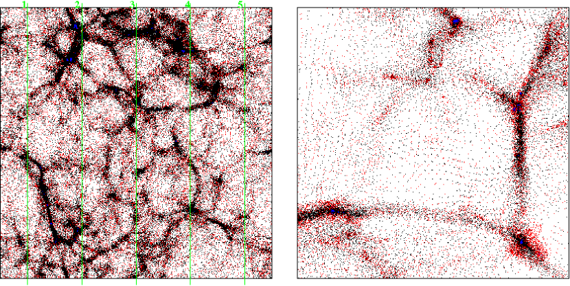
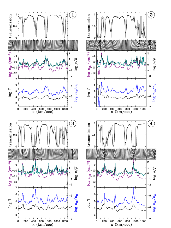
Figure 4 shows how density, temperature, velocity, and thermal broadening combine to produce Ly$\alpha$ forest spectra, along the sightlines marked 1–4 in Figure 3. In each panel, the bottommost plot shows the gas temperature in black and the neutral hydrogen fraction in blue. Because $n_{\mbox{\tiny HI}}/n_{\mbox{\tiny H}}\propto n_{\mbox{\tiny H}}T^{-0.7}$ and $T\propto n_{\mbox{\tiny H}}^{0.6}$ for gas on the $T$-$\rho$ relation, the neutral fraction and temperature are positively correlated at most temperatures. However, high temperature gas has usually been shock heated off the $T$-$\rho$ relation, and the recombination coefficient $\alpha_{\mbox{\tiny HII}}$ falls more steeply than $T^{-0.7}$ at high temperature (Katz et al., 1996), causing the neutral fraction to decrease dramatically (see, e.g., the feature near 100 km s^-1 in sightline #2). In the middle graphs, we plot the neutral hydrogen number density [cm^-3] in purple, using the scale on the left-hand axis. The gas and dark matter overdensities are plotted in black and cyan, respectively, using the scale on the right-hand axis. In general, the dark matter and gas overdensities are similar, but the dark matter has sharper, higher overdensity peaks as was seen visually in Figure 3. As expected from the $T$-$\rho$ relation, the gas overdensity and the gas temperature follow one another except at very high gas overdensity. The highest gas overdensities correspond to condensed halos—i.e., galaxies—and thus the gas has cooled to lower temperatures in these regions. The neutral hydrogen density shows more variation than the gas density because it is proportional $n_{\mbox{\tiny H}}^{2}$ (actually $\rho^{1.6}$ once temperature effects are included). The topmost plot has the transmitted flux $F\equiv\exp(-\tau_{\mbox{\tiny HI}})$ in black and the transmitted flux that would be observed in the absence of thermal broadening in grey. The lines between the middle plot and the top plot show the effects of peculiar velocities when converting from neutral hydrogen density in physical space to an observable flux in velocity space. Features contracting along the line of sight cause physically distinct gas regions to converge to the same region of the observed spectrum. However, if the connecting lines do not cross, then the region still has net expansion. Both the thermally broadened and non-thermally broadened spectra have the same characteristic broad features, implying that residual Hubble flow dominates the velocity width of these features. However, thermal broadening smooths the small scale roughness. At velocity caustics (converging lines in Figure 4), peculiar velocities cancel the Hubble flow, and the features do become narrower when one removes the thermal broadening.

Figure 4: Physical quantities and Ly$\alpha$ forest spectra along four of the sightlines labelled in Figure 3; velocity $v=0$ corresponds to the top of Figure 3. Shown in real space are the temperature (black, bottom), the neutral hydrogen fraction (blue, bottom), the H I number density (purple, middle), the gas overdensity (black, middle), and the dark matter overdensity (cyan, middle). The bars separating the top and middle panels show the effects of peculiar velocities when transitioning from real space to the observed flux transmission with (top, black) and without (top, grey) thermal broadening. See § 3.3 for more details.

3.4 Impacts of temperature and pressure on gas evolution

The obvious consequence of having a higher photoionization heating rate is that gas temperatures in the H4 simulation are higher than in the fiducial simulation, as shown at $z=3$ in the top panels of Figure 5. A more subtle effect, is that the larger Jeans length of the H4 simulation smooths the gas distribution, as shown in the density-coded bottom panels of Figure 5. There is a relative paucity of very dense clumps in the H4 simulation; this is especially noticeable in the lower density filaments.

Figure 5: Temperature (top) and density (bottom) evolution for gas particles in a $2.5\times 2.5\times 0.05$ $h^{-1}$ Mpc comoving slice at $z=3$ in the fiducial (left) and H4 (right) simulations. The temperature scale runs logarithmically from from $\log T=3.5$ (black/dark blue) to $\log T=5.5$ (yellow/white). The density scale runs from $\log(\rho_{\mbox{\scriptsize gas}}/\bar{\rho}_{\mbox{\scriptsize gas}})\equiv\log(1+\delta)=-1.3$ (black) to $\log(1+\delta)=1.3$ (green).

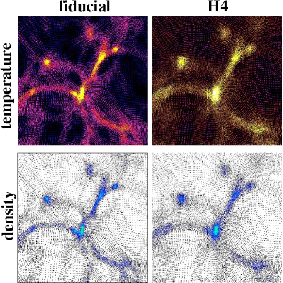
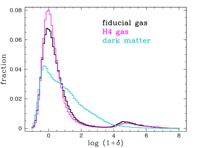
Figure 6 plots the distribution of gas overdensity in the fiducial and H4 simulations. The visual differences in the right panel of Figure 5 manifest themselves as a higher frequency of particles with $\rho_{\rm gas}/\bar{\rho}_{\rm gas}\sim 10$–100 in the fiducial simulation and a higher frequency of $\rho_{\rm gas}/\bar{\rho}_{\rm gas}\sim 1$ particles in the H4 simulation. This difference leads to a cancellation in many of the statistical comparisons in § 4; though the H4 gas is hotter (and thus has more thermal broadening), its higher pressure implies that there there is relatively less high-density and therefore relatively higher-temperature gas. For comparison, we also show in Figure 6 the density distribution of the dark matter, with densities computed using the SPH smoothing kernel. Because the dark matter is pressureless, it typically reaches higher overdensities, though it does not achieve the highest overdensities seen in the gas distributions because these arise from dissipation, i.e. cooling. Extrapolating from the density distributions in our low-resolution simulation, the dark matter density distribution would probably be somewhat less skewed if we increased the mass resolution of the simulation, but at low overdensity the gas distributions are essentially converged since we resolve the Jeans mass.

Figure 6: Distributions of gas overdensities at $z=3$ in the fiducial (black) and H4 (pink) simulations, as well as the dissipationless dark matter (cyan) in the fiducial simulation.

4 Effects of pressure and thermal broadening on the Ly$\alpha$ forest

To isolate the effects of gas pressure and thermal broadening in our subsequent analyses, we examine both the original gas particle distributions and distributions with one of the three imposed $T$-$\rho$ relations illustrated in Figure 1. For an imposed $T$-$\rho$ relation, we replace each gas particle’s temperature by the temperature that corresponds to its overdensity. We use the same procedure to create Ly$\alpha$ forest spectra from the dark matter distribution (“gasifying” the dark matter). The fiducial $T$-$\rho$ relation (yellow in Figure 1) matches that found for the IGM in the fiducial simulation; above $1+\delta=10$, the gas is “shock heated” to a temperature of $5\times 10^{5}$ K. Likewise, the pink lines in Figure 1 show the $T$-$\rho$ relation used to mimic the H4 simulation. Figure 6 shows that gas distributions with different pressure also sample the $T$-$\rho$ relation differently, and if the $T$-$\rho$ relation is sloped they will therefore experience different thermal broadening For example, using the fiducial $T$-$\rho$ relation, the H4 simulation would have less high density gas with large thermal broadening, and the dark matter distribution would have more. We, therefore, consider an additional, flat $T$-$\rho$ relation, with $T=2\times 10^{4}\,$K at all densities, so that we can examine the effects of pressure in the presence of pressure-independent thermal-broadening.

We now turn to the effects of pressure support and the $T$-$\rho$ relation on the Ly$\alpha$ forest spectra (§ 4.1) and on flux statistics (the flux power spectrum, § 4.2; the autocorrelation function, § 4.3; and the probability distribution function, § 4.4. For all these analyses we use the same sightlines in each simulation to ensure the effects of sample are variance the same.

4.1 Spectra

Figure 7 shows how pressure and the $T$-$\rho$ relation affect the Ly$\alpha$ spectra along the five sightlines labelled in Figure 3, with sightline #1 corresponding to the topmost spectrum in each panel; as in Figure 4, $v=0$ corresponds to the top of Figure 3. Any differences between the models are usually most noticeable in unsaturated lines. The top-left panel shows spectra computed directly from the simulated gas distributions, with differences in pressure support, differences in thermal broadening because of the different $T$-$\rho$ normalization, and differences in thermal broadening because of the sampling of the $T$-$\rho$ relation. Light grey lines show spectra from our lower resolution simulation. The impact of resolution is generally very small, but there are some slight differences.

There are two notable differences between the fiducial and H4 spectra exemplified by the $v\sim 450$ km s^-1 feature in sightline #5 and the $v\sim 750$ km s^-1 feature in sightline #4. First, features in the H4 spectra are broader than in the fiducial spectra, which could arise because of greater thermal broadening and/or because of the larger Jeans scale (and thus the larger $H\lambda_{J}$). Second, features in the H4 spectra are not as deep as in the fiducial case because the hotter gas does not reach as high overdensity and/or because higher thermal broadening smears out inherently sharp features.

Figure 7: Comparison of spectra along the sightlines labelled in Figure 3, isolating different physical effects. Top left: full effects of thermal broadening, thermal history and resolution are shown. Top right: effects of thermal broadening are isolated. Bottom left: effects of pressure support are isolated. Bottom right: effects of pressure support and different samplings of the underlying overdensity distribution are isolated. See § 4.1 for details.

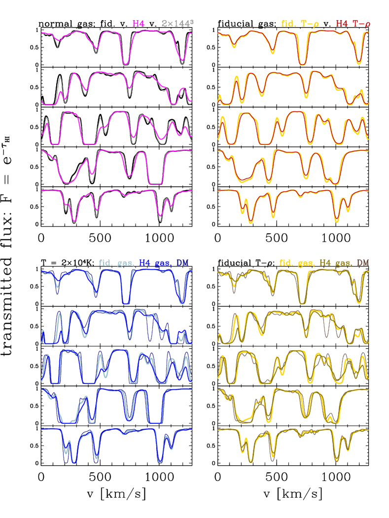
The top right panel isolates the impact of thermal broadening, applying the fiducial and H4 $T$-$\rho$ relations to the gas distribution of the fiducial simulation. The lower-left panel isolates the impact of pressure, applying the flat $T$-$\rho$ relation to the fiducial and H4 gas distributions and to the dark matter distribution from the fiducial simulation. In some cases, such as the $v\sim 150$ km s^-1 feature in sightline #1, the $v\sim 1025$ km s^-1 feature in sightline #3, and the $v\sim 250$ km s^-1 feature in sightline #4, differences in the full simulation spectra (upper left) are largely erased in the upper right panel but remain similar in the lower left panel, which shows that they mostly arise from different pressure effects in the two simulations rather than from differences in the thermal broadening. There are fewer cases of the reverse, where differences present in the full spectra remain in the upper right panels but disappear in the lower left, though some are visible in sightline #5. The differences in the upper-right (thermal broadening isolated) are always systematic, with lower thermal broadening yielding deeper and slightly narrower features. The differences between the H4 and fiducial gas distributions in the lower-left (pressure isolated) are more random, and we will see below that their statistical signature is weaker.

The pressureless dark matter distribution does lead to spectra with more small scale structure, as shown by the thin dark lines in the lower left. However, despite the clear differences between the gas and dark matter distributions evident in Figures 3, 4, and 6, the differences in the spectra created from these distributions are small. In the absence of thermal broadening, dark matter spectra are much more jagged than their gas counterparts shown in Figure 4, but realistic thermal broadening masks these differences to a large extent. The velocity widths of most features are not sensitive to the level of thermal broadening (as seen in the upper right) but neither are they set by the Jeans scale, or else the dark matter and gas spectra would have greater differences. Instead, thermal broadening erases the finest scale structures in the density field so that typical features correspond to coherent, moderate overdensity structures expanding with the Hubble flow.

Adopting the fiducial $T$-$\rho$ relation in place of the flat $T$-$\rho$ relation (bottom right) makes only a small difference to the usual appearance of the spectra (top left). Features that are flat-bottomed in the dark matter spectra with the flat $T$-$\rho$ relation often become less saturated with the fiducial $T$-$\rho$ relation, such as the $v\sim 775$ km s^-1 feature in sightline #3 and the $v\sim 1000$ km s^-1 feature in sightline #5. In these regions, the dark matter overdensity is high, so with $T\propto(1+\delta)^{0.6}$ they have higher thermal broadening, which spreads the feature in velocity space and reduces its saturation. In some cases, such as the $v\sim 725$ km s^-1 feature of sightline #1, the wings of the dark matter feature become noticeably broader than those of the gas features because of the higher temperatures at higher overdensities.

4.2 The 1-D Flux Power Spectrum

The Lyman-$\alpha$ flux power spectrum is a powerful tool for probing the dark matter mass power spectrum on the smallest scales. Because of the high redshift, the continuous sampling of the line-of-sight density field, and the moderate overdensity of absorbing structures, the Ly$\alpha$ forest provides a more direct link to the linear theory power spectrum than other small-scale tracers. (Primary cosmic microwave background anisotropies are damped on these scales.) However, to infer information about the structure of the underlying dark matter, one must understand the thermal structure of the IGM, as the amplitude and the shape of the flux power spectrum are connected to the gas temperature-density relation via equation (3.2). The bias of the flux power spectrum, i.e., $b^{2}(k)=P_{F}(k)/P_{\rm lin}(k)$, is also influenced by non-linear gravitational evolution, thermal broadening, pressure support, peculiar velocities, and shock heating (Croft et al., 1998, 1999, 2002; Viel et al., 2004, 2008; McDonald et al., 2005).

Figure 8: The 1-D flux power spectrum at $z=4.0$ (top), $z=3.0$ (middle), and $z=2.4$ (bottom), with the fiducial simulation in black, the H4 simulation in pink, and the lower-resolution simulation in grey. For reference, we also show the flux power spectrum in the absence of thermal broadening for the fiducial gas (green) and the H4 gas (purple), as well as the observed flux power spectrum from McDonald et al. (2001, squares) and Croft et al. (2002, triangles).

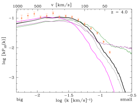
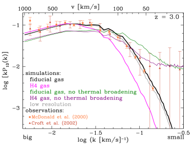
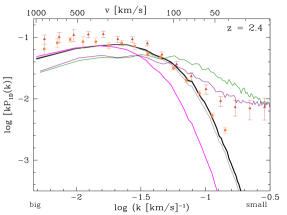
Figure 8 shows the one-dimensional line-of-sight flux power spectrum, $P_{\mbox{\scriptsize 1D}}(k)$ of $(F-\langle F\rangle)$, where $F\equiv\exp(-\tau_{\mbox{\tiny Ly}\alpha})$, based on 600 randomly selected sightlines through the fiducial, H4, and low resolution simulations. The flux power spectrum $P_{\mbox{\scriptsize 1D}}(k)$ is a measure of the variance of the flux, $\sigma_{\rm F}^{2}$, on different scales; specifically, we adopt the normalization convention of McDonald et al. (2000), where

$$\sigma_{F}^{2}=\int_{-\infty}^{\infty}\frac{{\rm d}k}{2\pi}P_{\mbox{\scriptsize 1D}}(k)=\pi^{-1}\int_{0}^{\infty}{\rm d}kP_{\mbox{\scriptsize 1D}}(k).$$ (8)

Also plotted in Figure 8 are the flux power spectra for the same lines of sight in both the fiducial and H4 simulations in the absence of thermal broadening. For reference, we also plot the observed flux power spectrum measured from high-resolution spectra given in Table 4 of McDonald et al. (2000, squares) and Table 7 (the “B” sample at $z=2.4$ and the “D” sample at $z=3$) of Croft et al. (2002, triangles). We have renormalized the Croft et al. (2002) measurements by McDonald et al.’s $\langle F\rangle^{2}$ to match our normalization convention.

The cutoff in the flux power spectrum at large $k$ is a consequence of thermal broadening, as is obvious from comparing the power spectra with and without thermal broadening. With thermal broadening included, the low resolution ($144^{3}$ gas particles) and fiducial ($288^{3}$) simulations produce very similar power spectra, indicating that even the lower resolution simulation is well converged for this statistic. At high $k$, the power spectra of the H4 simulation are offset by roughly a factor of $1.6$ in $k$ from the fiducial simulation, roughly consistent with the difference of 2–$2.5$ in $T_{0}$ (since thermal velocities scale as $T_{0}^{1/2}$). The cutoff scale in the fiducial simulation agrees better with the observational data, even though its temperatures are low compared to the McDonald et al. (2001) estimates (see Fig. 2).

Our cutoff scale also differs from that of Lidz et al. (2009, Figure 5); the flux power spectrum of our fiducial simulation is more similar (on small and large scales) to that of their hotter, $T_{0}=2\times 10^{4}$ K and $\alpha=0.3$, simulation than to their colder, $T_{0}=1\times 10^{4}$ K and $\alpha=0.6$, simulation, which has a $T$-$\rho$ relation similar to our fiducial simulation. We see no obvious reason for this discrepancy: the resolution test in Figure 8 shows good convergence, we do not expect the cutoff scale to be sensitive to box size, we have checked that high as density peaks produce the expected thermally broadened line profiles in our extracted spectra, and we find good agreement between the flux power spectrum from our $z=3$ spectra measured by our code (written by R. Croft) and an independent code written by P. McDonald. When spectra are extracted from our simulation using Lidz et al.’s code, the calculated $P(k)$ is consistent with the one we measure; the difference is therefore present in the simulated gas distributions themselves. For now, we draw no strong conclusions from the comparison to data in Figure 8, and focus instead on the relative roles of pressure support and thermal broadening.

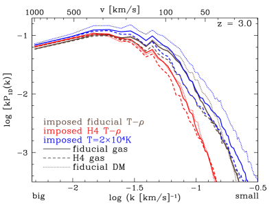
To separate the effects of gas pressure and thermal broadening, Figure 9 shows $z=3$ flux power spectra from 200 randomly selected sightlines through the fiducial gas, H4 gas, and fiducial dark matter density fields (indicated by the line type), each with three imposed temperature-density relations: fiducial, H4, and flat (indicated by the line color). Comparing lines of the same color in Figure 9 shows the effects of pressure support, with the same $T$-$\rho$ relation applied to different density distributions. Comparing lines of the same type but different colors isolates the effect of the $T$-$\rho$ relation for the same underlying density distribution. The lines clearly separate into three groups based on color, showing that thermal broadening dominates over pressure support in determining the scale of the power spectrum cutoff. There is some difference among the three density distributions when we impose a constant IGM temperature $T=2\times 10^{4}$ K (blue lines), which shows that some of the similarity for the other $T$-$\rho$ relations may reflect the cancellation discussed in § 3.4, where the distribution with a larger Jeans length has less high density gas to experience high thermal broadening. However, on the whole our results confirm the finding of McDonald (2003) that it is the instantaneous $T$-$\rho$ relation (at the epoch of observation) rather than the detailed gas thermal history (and thus pressure history) that determines the $P_{F}(k)$ cutoff.

Figure 9: The 1-D flux power spectrum at $z=3$ for fiducial gas (solid lines), H4 gas (dashed lines), and fiducial dark matter (dotted lines) with fiducial (brown), H4 (red), and flat (blue) imposed temperature-density relations.

4.3 Flux Decrement Autocorrelation Functions

The flux decrement autocorrelation function,

$$\xi_{\mbox{\scriptsize auto}}(\Delta v)\equiv\frac{\langle D(v)D(v+\Delta v)\rangle}{\langle D\rangle^{2}},$$ (9)

is a commonly used tool for characterizing the Ly$\alpha$ forest. While technically the one-dimensional flux power spectrum and flux autocorrelation functions codify the same information ($P_{F}(k)$ is just the one-dimensional Fourier transform of $\xi_{\mbox{\scriptsize auto}}$), the flux autocorrelation function is often easier to describe both observationally and from simulations because its definition does not depend on information from all scales. Furthermore, as cross-correlation functions are more typically used to describe information in closely paired lines of sight than cross-power spectra, it is important for us to understand the effects of pressure and temperature on the autocorrelation function before examining paired sightlines (in Paper II).

Figure 10: Left: Normalized flux decrement autocorrelation functions, $\xi_{\mbox{\scriptsize auto}}\equiv\langle D(v)D(v+\Delta v)\rangle/\langle D\rangle^{2}$, at $z=2.4,\,3.0$, and 4.0. The black curve with error bars shows results for the fiducial simulation, while the pink and grey lines show results for the H4 and low-resolution simulations, respectively. Red and mustard lines show, respectively, the fiducial gas with the H4 $T$-$\rho$ relation imposed and the H4 gas with the fiducial $T$-$\rho$. The green line shows the fiducial gas with no thermal broadening. Right: Normalized $\xi_{\mbox{\scriptsize auto}}$, for the fiducial gas (light blue), H4 gas (bright blue), and fiducial dark matter (dark blue), all with an imposed temperature of $T=2\times 10^{4}$ K.

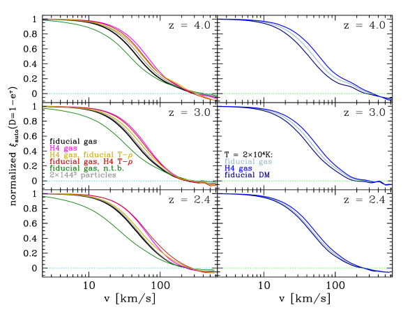
Figure 10 plots normalized flux decrement autocorrelation functions at $z=2.4$, 3.0, and 4.0. We normalize $\xi_{\rm auto}=1$ at the smallest scales to highlight differences in the turnover scale of the correlation function rather than differences in normalization. The fiducial and low-resolution simulations have nearly identical $\xi_{\rm auto}$, while the H4 simulation has a noticeably larger coherence scale. However, if we impose the fiducial $T$-$\rho$ relation on the H4 gas, then $\xi_{\rm auto}$ is nearly identical to that of the fiducial simulation. Conversely, imposing the H4 $T$-$\rho$ on the fiducial simulation yields nearly the same $\xi_{\rm auto}$ as the H4 simulation.

While these results suggest that the effects of pressure are small compared to those of thermal broadening, the right-hand panels of Figure 10 show that $\xi_{\rm auto}$ is different for the H4 gas, fiducial gas, and fiducial dark matter if we impose a flat $T=2\times 10^{4}$ K on all particles. In this case, the higher pressure distribution exhibits a larger coherence scale, especially at high redshifts. Thus, the similarity of the fiducial and H4 distributions with the same imposed $T$-$\rho$, seen in the left-hand panels, arises partly from the counter-balancing effects of $T_{0}$ and the changes in the distribution of gas densities discussed in § 3.4 (see Figure 6).

4.4 Flux Decrement Probability Distributions

The flux decrement probability distribution function (PDF) is a potentially powerful tool for probing the IGM, both by itself and as a means of adding constraints to other statistical measures such as the flux power spectrum (Rauch et al., 1997; Weinberg, 1999; Gaztañaga & Croft, 1999; Nusser & Haehnelt, 2000; Desjacques & Nusser, 2005; Desjacques et al., 2007). In particular, Bolton et al. (2008) have recently used the Ly$\alpha$ forest flux distribution as measured by Kim et al. (2007) to suggest that the temperature-density relation at $z\sim 3$ is inverted ($\alpha<0$ in equation 5), with low-density gas at higher temperature than higher density gas. While the differences owing to changes in the $T$-$\rho$ relation are not as extreme as those in $P_{F}(k)$ or $\xi_{\mbox{\scriptsize auto}}$, the flux decrement PDF can potentially be measured to much higher accuracy using the same number of sightlines. On the other hand, the PDF is sensitive to continuum fitting, while on small scales $P_{F}(k)$ is not (on large scales continuum fitting can be problematic even for $P_{F}(k)$; e.g., Kim et al. 2004). Furthermore, high-resolution spectra are needed to accurately measure the PDF (Viel et al., 2004; Tytler et al., 2004). Since high-resolution spectra will always exist in smaller numbers than low-resolution spectra, it should be noted that the PDF is also potentially sensitive to sample variance, the explanation Kim et al. (2007) suggest for the $\sim$30% difference between their $z\sim 3$ PDF and the one measured by McDonald et al. (2000) on a very similar data set.

Figure 11: Flux decrement probability distributions in linear bins of $D$ at $z=2.4$, 3, and 4 for the fiducial and H4 simulations, with (black and pink) inherent temperatures and imposed H4 (red) and fiducial (mustard) $T$-$\rho$ relations, respectively. The points at $z=2.4$ and 3 are included to show the $p(D)$ in the most transparent (left) and opaque (right) bins.

Figure 12: Flux decrement probability distributions in logarithmic bins of $D$ at $z=2.4$, 3, and 4 for the fiducial gas distribution, with inherent temperatures (black), at low resolution (grey), and with imposed H4 $T$-$\rho$ (red). Also shown are the imposed H4 gas distribution with inherent temperatures (pink), with the imposed fiducial $T$-$\rho$ (mustard), as well as both the fiducial and H4 gas distributions with an imposed flat $T=2\times 10^{4}$ K (light blue and bright blue, respectively). The points are included to show the $p(D)$ in the final (most opaque) bin.

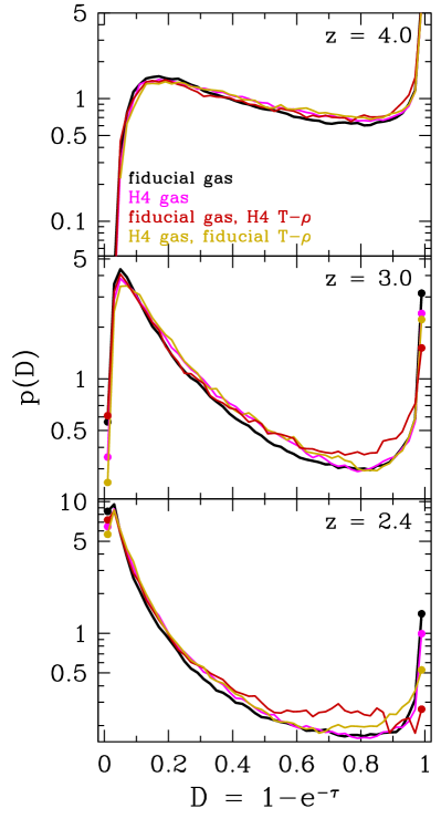
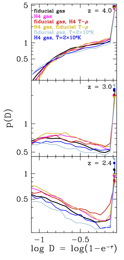
Figure 11 shows the linear flux decrement PDF, i.e., $p(D)$, where $p(D)\Delta D$ is the number of pixels in a bin of width $\Delta D$ divided by the total number of pixels. In Figure 12 we show for a larger set of models the logarithmic PDF, $p(\log D)$, which allows better visual discrimination in the range $0.1<D<0.5$. The shape of the PDF changes radically with redshift as the mean flux decrement changes; physically, this change is driven by the mean density dropping as $(1+z)^{3}$. However, as all the models at a given redshift are normalized to the same $\langle D\rangle$, the effects of $T$-$\rho$ changes on the mean absorption are removed. Though for visual clarity we do not plot the PDFs from the $2\times 144^{3}$ particle simulation, the low resolution and fiducial PDFs differ by $\sim$1–5%; this difference is much smaller than the typical model differences in Figures 11 and 12.

Thermal broadening reduces the number of transparent ($D\approx 0$) pixels, while pressure support increases the number of pixels at extreme flux decrements (for visual clarity, we do not plot the dark matter and non-thermally broadened PDFs). At all redshifts, the spectra generated from the full H4 simulation have more pixels with mid-range flux decrements, i.e. relative to the fiducial simulation, the H4 simulation produces fewer opaque pixels and fewer transparent pixels. This is as expected, since higher pressure smooths the gas distribution and higher temperature leads to greater thermal broadening. However, the fiducial simulation with the imposed H4 $T$-$\rho$ has fewer saturated pixels than the H4 simulation itself, and more pixels with $D\approx 0.6$–$0.8$. This surprising result highlights the sometimes complicated interplay between the density distribution and the $T$-$\rho$ relation. The fiducial simulation has more high overdensity gas (Figure 6), but because this gas is at high temperature (with $T\propto[1+\delta]^{0.6}$), thermal broadening converts narrow, fully saturated features to broader, moderately saturated ones.

The slope of the $T$-$\rho$ relation has a direct impact on the flux PDF, independent of thermal broadening, because it affects the mapping from density contrast to flux. Equation (3.2) gives $\tau_{\mbox{\tiny HI}}\propto(1+\delta)^{2-0.7\alpha}$, so $\tau_{\mbox{\tiny HI}}\propto(1+\delta)^{1.6}$ for our fiducial and H4 relations (with $\alpha\approx 0.6$) and $\tau_{\mbox{\tiny HI}}\propto(1+\delta)^{2}$ for our flat, $T=2\times 10^{4}$ K relation ($\alpha=0$). Imposing a constant $T$ substantially alters the PDFs of both the fiducial and H4 simulations (blue curves in Figure 12), with the greater sensitivity of $\tau_{\mbox{\tiny HI}}$ to $(1+\delta)$ leading to more saturated pixels and fewer mid-range pixels. The two simulations have significantly different PDFs, which with constant thermal broadening must arise from effects of pressure on the gas density distribution. In contrast to the power spectrum and flux correlation function, thermal broadening and pressure support have comparable impact on the flux PDF, and they interact in complex ways. This different behavior arises because the PDF responds directly to the full overdensity distribution and its mapping to flux, while the power spectrum and correlation function measure the variance of this distribution as a function of scale.

5 Conclusions

We have investigated the relative importance of pressure support and thermal broadening in determining the longitudinal structure of the Lyman-$\alpha$ forest. Our main results come from comparing two SPH simulations with identical initial conditions but different photoionization heating rates, which produce a factor of $\sim 2.3$ difference in the temperature of diffuse IGM gas. We have imposed different temperature-density relations on the simulation outputs to isolate physical effects, extracted spectra from the dark matter distribution to extend our investigation to the pressureless case, and compared the fiducial simulation ($2\times 288^{3}$ particles) to a lower resolution simulation ($2\times 144^{3}$) to quantify numerical resolution effects.

Equation (1) shows that the Hubble flow across the Jeans scale is generally of the same magnitude as thermal broadening ($H\lambda_{J}\sim\sigma_{\rm th}$). However, the IGM is an expanding, inhomogeneous medium evolving in the potential of a non-linear dark matter distribution, so the Jeans length is at best an approximate description of the scale imposed by gas pressure support. It is therefore difficult to know without detailed simulations whether thermal broadening or pressure support will dominate the structure of the forest. A related question is the meaning of the density contrast $\delta$ in the fluctuating Gunn-Peterson approximation (equation 3.2). In principle, this should be the density of the gas that is absorbing Ly$\alpha$ photons, but analyses of early SPH simulations found that Ly$\alpha$ forest spectra created from the (pressureless) dark matter distribution were remarkably similar to those created from the (pressure supported) gas distribution (e.g., Croft et al., 1998). However, the relatively low resolution of those simulations (a mass resolution that is $\sim 60$ times lower than our fiducial simulation here) raised the possibility that both sets of spectra were artificially broadened to the numerical resolution limit. We investigate this issue more confidently here because the initial particle spacing of our $288^{3}$ simulations, $43\,h^{-1}$ kpc comoving, is far below the typical Jeans length at IGM overdensities, $\lambda_{J}\sim\,800h^{-1}$ kpc comoving, and because our $144^{3}$ simulation allows a direct resolution test.

In broad brush, our conclusions are that thermal broadening dominates over pressure support in determining the visual appearance and statistical properties of the Ly$\alpha$ forest, but that differences in gas pressure do have a noticeable effect. The widths of absorption features are typically set by Hubble flow across the absorbing structure, though thermal broadening does smooth out small scale corrugations to create coherent features (see Fig. 4). Once we include thermal broadening, the spectra created from dark matter distributions are similar to those created from the gas, even though the effects of pressure support on the gas density field are readily discernible. Thus, one can drastically change the Jeans scale without drastically changing the forest. However, dark matter spectra are visually and statistically distinguishable from gas spectra, more so than in the earlier generation of lower resolution SPH simulations.

Turning to individual statistics, we find that thermal broadening sets the turnover scale of the one-dimensional flux power spectrum, with the fiducial gas, H4 gas, and dark matter distributions producing similar power spectra if one imposes the fiducial or H4 $T$-$\rho$ relation on all three. Similar conclusions hold for the coherence scale of the flux decrement autocorrelation function. However, in both cases, the weak impact of pressure support partly owes to a cancellation effect that arises with a sloped $T$-$\rho$ relation: a higher pressure distribution has more “Jeans broadening,” but it has less thermal broadening because there is less high overdensity, high temperature gas. When we impose a constant IGM temperature of $T=2\times 10^{4}$ K, the differences among the three cases are more noticeable, though they are still small compared to the effects of thermal broadening. For the flux decrement probability distribution function, thermal broadening and pressure support have effects of comparable magnitude, though thermal broadening is still somewhat more important.

Our $144^{3}$ and $288^{3}$ simulations yield similar results for all our statistics. The resolution effects are larger at $z=4$ than at lower redshifts, where they have a small but noticeable impact on all the statistics. For most purposes, the resolution of our $144^{3}$ simulations (in a $12.5\,h^{-1}$ Mpc comoving volume) is adequate.

Though it is a stronger player than pressure support in setting the scale of the longitudinal Ly$\alpha$ forest, thermal broadening is an inherently one-dimensional phenomenon. Because pressure acts in three dimensions, we expect it to play the main role in setting the transverse coherence of the Ly$\alpha$ forest across neighboring sightlines. Growing samples of binary quasars with separations of $\Delta\theta\lesssim 10$″ now make it possible to probe the expected Jeans scale (Hennawi et al., 2006, 2009). We show in Paper II that the degree of transverse coherence on these scales is indeed sensitive to gas pressure support and insensitive to thermal broadening. Observational studies of close quasar pairs can directly probe the scale of pressure support on the Lyman-$\alpha$ forest, providing new insights into the physical state and thermal history of the high-redshift intergalactic medium.

References

- Bertone & White (2006) Bertone, S. & White, S. D. M. 2006, MNRAS, 367, 247
- Bi & Davidsen (1997) Bi, H. & Davidsen, A. F. 1997, ApJ, 479, 523
- Bolton et al. (2008) Bolton, J. S., Viel, M., Kim, T.-S., Haehnelt, M. G., & Carswell, R. F. 2008, MNRAS, 386, 1131
- Cen et al. (1994) Cen, R., Miralda-Escudé, J., Ostriker, J. P., & Rauch, M. 1994, ApJL, 437, L9
- Coles & Jones (1991) Coles, P. & Jones, B. 1991, MNRAS, 248, 1
- Croft et al. (2002) Croft, R. A. C., Weinberg, D. H., Bolte, M., Burles, S., Hernquist, L., Katz, N., Kirkman, D., & Tytler, D. 2002, ApJ, 581, 20
- Croft et al. (1997) Croft, R. A. C., Weinberg, D. H., Katz, N., & Hernquist, L. 1997, ApJ, 488, 532
- Croft et al. (1998) —. 1998, ApJ, 495, 44
- Croft et al. (1999) Croft, R. A. C., Weinberg, D. H., Pettini, M., Hernquist, L., & Katz, N. 1999, ApJ, 520, 1
- Davé et al. (1999) Davé, R., Hernquist, L., Katz, N., & Weinberg, D. H. 1999, ApJ, 511, 521
- Desjacques & Nusser (2005) Desjacques, V. & Nusser, A. 2005, MNRAS, 361, 1257
- Desjacques et al. (2007) Desjacques, V., Nusser, A., & Sheth, R. K. 2007, MNRAS, 374, 206
- Fan et al. (2006) Fan, X., Carilli, C. L., & Keating, B. 2006, ARA&A, 44, 415
- Furlanetto & Oh (2008) Furlanetto, S. R. & Oh, S. P. 2008, ApJ, 682, 14
- Gaztañaga & Croft (1999) Gaztañaga, E. & Croft, R. A. C. 1999, MNRAS, 309, 885
- Gnedin & Hui (1998) Gnedin, N. Y. & Hui, L. 1998, MNRAS, 296, 44
- Gunn & Peterson (1965) Gunn, J. E. & Peterson, B. A. 1965, ApJ, 142, 1633
- Haardt & Madau (2001) Haardt, F. & Madau, P. 2001, in Clusters of Galaxies and the High Redshift Universe Observed in X-rays, ed. D. M. Neumann & J. T. V. Tran
- Hennawi et al. (2009) Hennawi, J. F., Myers, A. D., Shen, Y., Strauss, M. A., Djorgovski, S. G., Fan, X., Glikman, E., Mahabal, A., Martin, C. L., Richards, G. T., Schneider, D. P., & Shankar, F. 2009, ArXiv:0908.3907
- Hennawi et al. (2006) Hennawi, J. F., Strauss, M. A., Oguri, M., Inada, N., Richards, G. T., Pindor, B., Schneider, D. P., Becker, R. H., Gregg, M. D., Hall, P. B., Johnston, D. E., Fan, X., Burles, S., Schlegel, D. J., Gunn, J. E., Lupton, R. H., Bahcall, N. A., Brunner, R. J., & Brinkmann, J. 2006, AJ, 131, 1
- Hernquist et al. (1996) Hernquist, L., Katz, N., Weinberg, D. H., & Miralda-Escudé, J. 1996, ApJL, 457, L51+
- Hinshaw et al. (2009) Hinshaw, G., Weiland, J. L., Hill, R. S., Odegard, N., Larson, D., Bennett, C. L., Dunkley, J., Gold, B., Greason, M. R., Jarosik, N., Komatsu, E., Nolta, M. R., Page, L., Spergel, D. N., Wollack, E., Halpern, M., Kogut, A., Limon, M., Meyer, S. S., Tucker, G. S., & Wright, E. L. 2009, ApJS, 180, 225
- Hui & Gnedin (1997) Hui, L. & Gnedin, N. Y. 1997, MNRAS, 292, 27
- Hui & Haiman (2003) Hui, L. & Haiman, Z. 2003, ApJ, 596, 9
- Katz et al. (1996) Katz, N., Weinberg, D. H., & Hernquist, L. 1996, ApJS, 105, 19
- Kim et al. (2004) Kim, T., Viel, M., Haehnelt, M. G., Carswell, R. F., & Cristiani, S. 2004, MNRAS, 347, 355
- Kim et al. (2007) Kim, T.-S., Bolton, J. S., Viel, M., Haehnelt, M. G., & Carswell, R. F. 2007, MNRAS, 382, 1657
- Kollmeier et al. (2006) Kollmeier, J. A., Miralda-Escudé, J., Cen, R., & Ostriker, J. P. 2006, ApJ, 638, 52
- Lidz et al. (2009) Lidz, A., Faucher-Giguere, C. ., Dall’Aglio, A., McQuinn, M., Fechner, C., Zaldarriaga, M., Hernquist, L., & Dutta, S. 2009, ArXiv:0909.5210
- Lynds (1971) Lynds, R. 1971, ApJL, 164, L73+
- Marble et al. (2008) Marble, A. R., Eriksen, K. A., Impey, C. D., Oppenheimer, B. D., & Davé, R. 2008, ApJ, 675, 946
- McDonald (2003) McDonald, P. 2003, ApJ, 585, 34
- McDonald et al. (2001) McDonald, P., Miralda-Escudé, J., Rauch, M., Sargent, W. L. W., Barlow, T. A., & Cen, R. 2001, ApJ, 562, 52
- McDonald et al. (2000) McDonald, P., Miralda-Escudé, J., Rauch, M., Sargent, W. L. W., Barlow, T. A., Cen, R., & Ostriker, J. P. 2000, ApJ, 543, 1
- McDonald et al. (2006) McDonald, P., Seljak, U., Burles, S., Schlegel, D. J., Weinberg, D. H., Cen, R., Shih, D., Schaye, J., Schneider, D. P., Bahcall, N. A., Briggs, J. W., Brinkmann, J., Brunner, R. J., Fukugita, M., Gunn, J. E., Ivezić, Ž., Kent, S., Lupton, R. H., & Vanden Berk, D. E. 2006, ApJS, 163, 80
- McDonald et al. (2005) McDonald, P., Seljak, U., Cen, R., Shih, D., Weinberg, D. H., Burles, S., Schneider, D. P., Schlegel, D. J., Bahcall, N. A., Briggs, J. W., Brinkmann, J., Fukugita, M., Ivezić, Ž., Kent, S., & Vanden Berk, D. E. 2005, ApJ, 635, 761
- McQuinn et al. (2009) McQuinn, M., Lidz, A., Zaldarriaga, M., Hernquist, L., Hopkins, P. F., Dutta, S., & Faucher-Giguère, C.-A. 2009, ApJ, 694, 842
- Meiksin & White (2001) Meiksin, A. & White, M. 2001, MNRAS, 324, 141
- Miralda-Escude (1993) Miralda-Escude, J. 1993, MNRAS, 262, 273
- Miralda-Escudé et al. (1996) Miralda-Escudé, J., Cen, R., Ostriker, J. P., & Rauch, M. 1996, ApJ, 471, 582
- Miralda-Escudé & Rees (1994) Miralda-Escudé, J. & Rees, M. J. 1994, MNRAS, 266, 343
- Nusser & Haehnelt (2000) Nusser, A. & Haehnelt, M. 2000, MNRAS, 313, 364
- Rauch et al. (1997) Rauch, M., Miralda-Escude, J., Sargent, W. L. W., Barlow, T. A., Weinberg, D. H., Hernquist, L., Katz, N., Cen, R., & Ostriker, J. P. 1997, ApJ, 489, 7
- Reisenegger & Miralda-Escude (1995) Reisenegger, A. & Miralda-Escude, J. 1995, ApJ, 449, 476
- Ricotti et al. (2000) Ricotti, M., Gnedin, N. Y., & Shull, J. M. 2000, ApJ, 534, 41
- Sargent et al. (1980) Sargent, W. L. W., Young, P. J., Boksenberg, A., & Tytler, D. 1980, ApJS, 42, 41
- Schaye (2001) Schaye, J. 2001, ApJ, 559, 507
- Schaye et al. (1999) Schaye, J., Theuns, T., Leonard, A., & Efstathiou, G. 1999, MNRAS, 310, 57
- Schaye et al. (2000) Schaye, J., Theuns, T., Rauch, M., Efstathiou, G., & Sargent, W. L. W. 2000, MNRAS, 318, 817
- Springel (2005) Springel, V. 2005, MNRAS, 364, 1105
- Theuns et al. (1998) Theuns, T., Leonard, A., Efstathiou, G., Pearce, F. R., & Thomas, P. A. 1998, MNRAS, 301, 478
- Theuns et al. (2000) Theuns, T., Schaye, J., & Haehnelt, M. G. 2000, MNRAS, 315, 600
- Tytler et al. (2004) Tytler, D., Kirkman, D., O’Meara, J. M., Suzuki, N., Orin, A., Lubin, D., Paschos, P., Jena, T., Lin, W.-C., Norman, M. L., & Meiksin, A. 2004, ApJ, 617, 1
- Viel et al. (2008) Viel, M., Becker, G. D., Bolton, J. S., Haehnelt, M. G., Rauch, M., & Sargent, W. L. W. 2008, Physical Review Letters, 100, 041304
- Viel & Haehnelt (2006) Viel, M. & Haehnelt, M. G. 2006, MNRAS, 365, 231
- Viel et al. (2004) Viel, M., Haehnelt, M. G., & Springel, V. 2004, MNRAS, 354, 684
- Viel et al. (2002) Viel, M., Matarrese, S., Mo, H. J., Haehnelt, M. G., & Theuns, T. 2002, MNRAS, 329, 848
- Weinberg (1999) Weinberg, D. e. a. 1999, in Evolution of Large Scale Structure : From Recombination to Garching, ed. A. J. Banday, R. K. Sheth, & L. N. da Costa, 346–+
- Weinberg et al. (1997) Weinberg, D. H., Hernsquit, L., Katz, N., Croft, R., & Miralda-Escudé, J. 1997, in Structure and Evolution of the Intergalactic Medium from QSO Absorption Line System, ed. P. Petitjean & S. Charlot, 133–+
- Zaldarriaga et al. (2001) Zaldarriaga, M., Hui, L., & Tegmark, M. 2001, ApJ, 557, 519
- Zhang et al. (1995) Zhang, Y., Anninos, P., & Norman, M. L. 1995, ApJL, 453, L57+