Pressure Support vs. Thermal Broadening in the Lyman-α𝛼\alpha Forest II:
Effects of the Equation of State on Transverse Structure

Molly S. Peeples1, David H. Weinberg1, Romeel Davé2, Mark A. Fardal3, Neal Katz3
1Department of Astronomy and the Center for Cosmology and Astro-Particle Physics, The Ohio State University, Columbus, OH 43210
2University of Arizona, Steward Observatory, Tucson, AZ 85721
3Department of Astronomy, University of Massachusetts, Amherst, MA 01003
E-mail: molly@astronomy.ohio-state.edu
Abstract

We examine the impact of gas pressure on the transverse coherence of high-redshift (2z42𝑧42\leq z\leq 4) Lyman-α𝛼\alpha forest absorption along neighboring lines of sight that probe the gas Jeans scale (projected separation Δrp500h1Δsubscript𝑟𝑝500superscript1\Delta r_{p}\leq 500h^{-1} kpc comoving; angular separation Δθ30less-than-or-similar-toΔ𝜃30\Delta\theta\lesssim 30\arcsec). We compare predictions from two smoothed particle hydrodynamics (SPH) simulations that have different photoionization heating rates and thus different temperature-density relations in the intergalactic medium (IGM). We also compare spectra computed from the gas distributions to those computed from the pressureless dark matter. The coherence along neighboring sightlines is markedly higher for the hotter, higher pressure simulation, and lower for the dark matter spectra. We quantify this coherence using the flux cross-correlation function and the conditional distribution of flux decrements as a function of transverse and line-of-sight (velocity) separation. Sightlines separated by Δθ15less-than-or-similar-toΔ𝜃15\Delta\theta\lesssim 15\arcsec are ideal for probing this transverse coherence. Higher pressure decreases the redshift-space anisotropy of the flux correlation function, while higher thermal broadening increases the anisotropy. In contrast to the longitudinal (line-of-sight) structure of the Lyα𝛼\alpha forest, the transverse structure on these scales is dominated by pressure effects rather than thermal broadening. With the rapid recent growth in the number of known close quasar pairs, paired line-of-sight observations offer a promising new route to probe the IGM temperature-density relation and test the unexpectedly high temperatures that have been inferred from single sightline analyses.

keywords:
cosmology: miscellaneous — intergalactic medium — methods: numerical
pagerange: Pressure Support vs. Thermal Broadening in the Lyman-α𝛼\alpha Forest II: Effects of the Equation of State on Transverse StructureApubyear: 2009

1 Introduction

The 1.5z6less-than-or-similar-to1.5𝑧less-than-or-similar-to61.5\lesssim z\lesssim 6 intergalactic medium (IGM) is most commonly studied via the Lyman-α𝛼\alpha forest, which arises from Lyα𝛼\alpha absorption of neutral hydrogen along the line of sight to some distant source (e.g., a quasar). Most of the information we have on the nature of the IGM is from sightlines piercing physically distinct regions of the IGM. Absorption features have finite widths, but from individual sightlines it is difficult to separate the contribution of bulk velocities (Hubble flow and peculiar velocities) from those of thermal broadening. Close quasar pairs can break this degeneracy by probing the transverse structure of the IGM. In the mid-1990s, several studies of quasar groups and lensed quasars definitively showed that the absorbing structures are coherent over hundreds of kpc (Bechtold et al., 1994; Dinshaw et al., 1994; Fang et al., 1996; Charlton et al., 1997; Crotts & Fang, 1998; D’Odorico et al., 1998). These observations provided critical support for the physical picture of the Lyα𝛼\alpha forest then emerging from cosmological simulations (Cen et al., 1994; Zhang et al., 1995; Hernquist et al., 1996) and associated analytic descriptions (Rauch & Haehnelt, 1995; Reisenegger & Miralda-Escude, 1995; Bi & Davidsen, 1997; Hui et al., 1997), in which most Lyα𝛼\alpha absorption arises in a continuously fluctuating medium of low density gas rather than in a system of discrete clouds. More recently, observations of pairs have been suggested as ways of investigating measuring the cosmological constant via the Alcock & Paczynski (1979) effect (McDonald & Miralda-Escudé, 1999), the matter power spectrum on small scales (Viel et al., 2002), and the IGM temperature-density relation. It is on the last of these that we focus in this paper.

Theoretical models predict that the low density IGM should have a power-law “equation of state,”

T=T0(1+δ)α,𝑇subscript𝑇0superscript1𝛿𝛼T=T_{0}(1+\delta)^{\alpha}, (1)

with denser gas being hotter than less dense gas (α>0𝛼0\alpha>0, Katz et al., 1996; Miralda-Escudé et al., 1996; Hui & Gnedin, 1997). Although this temperature-density (T𝑇T-ρ𝜌\rho) relation is difficult to measure, multiple observations suggest that it has a higher normalization and a shallower slope than that expected using the most straightforward assumptions about photoionization heating (Schaye et al., 2000; McDonald et al., 2001; Theuns et al., 2002; Bolton et al., 2008). Because the degree of small-scale transverse coherence is set by the Jeans length, and the Jeans length depends on the temperature of the gas, studying the transverse structure of the Lyα𝛼\alpha forest might give insight into the IGM T𝑇T-ρ𝜌\rho relation (J. Hennawi, private communication, 2007). In Peeples et al. (2009, hereafter Paper I), we show that while thermal broadening and pressure support both affect the longitudinal structure of the Lyα𝛼\alpha forest, thermal broadening dominates. In this paper we investigate the effects of the temperature-density relation via pressure support and thermal broadening on the transverse small-scale structure of the Lyα𝛼\alpha forest.

The gas temperature affects the Jeans length λJsubscript𝜆𝐽\lambda_{J} (and the comoving Jeans length λJ,comvsubscript𝜆𝐽comv\lambda_{J,{\rm comv}}) via

λJsubscript𝜆𝐽\displaystyle\lambda_{J} \displaystyle\equiv csπGρsubscript𝑐𝑠𝜋𝐺𝜌\displaystyle c_{s}\sqrt{\frac{\pi}{G\rho}} (2)
λJ,comvabsentsubscript𝜆𝐽comv\displaystyle\Rightarrow\lambda_{J,{\rm comv}} =\displaystyle= (1+z)σthH015π3[38πΩm,0(1+z)3(1+δ)]1/21𝑧subscript𝜎thsuperscriptsubscript𝐻015𝜋3superscriptdelimited-[]38𝜋subscriptΩ𝑚0superscript1𝑧31𝛿12\displaystyle(1+z)\sigma_{\rm th}H_{0}^{-1}\sqrt{\frac{5\pi}{3}}\left[\frac{3}{8\pi}\Omega_{m,0}(1+z)^{3}(1+\delta)\right]^{-1/2}
=\displaystyle= 782h1kpc782superscript1kpc\displaystyle 782\,h^{-1}\,\mbox{kpc}
×(σth11.8kms1)[(Ωm,0(1+δ)0.25×(1+0))(1+z1+3)]1/2,absentsubscript𝜎th11.8kmsuperscripts1superscriptdelimited-[]subscriptΩ𝑚01𝛿0.25101𝑧1312\displaystyle\times\left(\frac{\sigma_{\rm th}}{11.8\,\rm{km}\,\rm{s}^{-1}}\right)\left[\left(\frac{\Omega_{m,0}(1+\delta)}{0.25\times(1+0)}\right)\left(\frac{1+z}{1+3}\right)\right]^{-1/2},

where 1+δρgas/ρ¯b1𝛿subscript𝜌gassubscript¯𝜌𝑏1+\delta\equiv\rho_{\rm gas}/\bar{\rho}_{b} is the gas overdensity and cs=[5kT]/[3m]=σth5/3subscript𝑐𝑠delimited-[]5𝑘𝑇delimited-[]3𝑚subscript𝜎th53c_{s}=\sqrt{[5kT]/[3m]}=\sigma_{\rm th}\sqrt{5/3} is the speed of sound in an ideal gas expressed as a multiple of the 1-D thermal velocity σthsubscript𝜎th\sigma_{\rm th}, which we have normalized to correspond to 104superscript10410^{4} K (Miralda-Escudé et al., 1996; Schaye, 2001; Desjacques & Nusser, 2005). While thermal broadening affects the observed IGM by smoothing the Lyα𝛼\alpha forest in one-dimension (namely, along the line of sight), pressure support smooths the physical gas distribution in all three dimensions. Therefore, while we found in Paper I that σthsubscript𝜎th\sigma_{\rm th} dominates the longitudinal Lyα𝛼\alpha forest structure, we expect λJsubscript𝜆𝐽\lambda_{J} to dominate the transverse structure. Our simulations indicate that the “effective” Jeans length in the Lyα𝛼\alpha forest is smaller than that given in Equation (1) by a factor of a few, probably owing to a combination of geometric factors, the universe expanding on the same timescale as the gas evolves, and the contribution of dark matter to the gravitational forces (see also Gnedin & Hui, 1998).

For Ωm=0.25subscriptΩ𝑚0.25\Omega_{m}=0.25 and ΩΛ=0.75subscriptΩΛ0.75\Omega_{\Lambda}=0.75, the relation between angular separation ΔθΔ𝜃\Delta\theta and comoving transverse separation R𝑅R at z=2𝑧2z=2–4 is approximately

Δθ4.4(1+z4)0.6×(R100h1kpc).Δ𝜃4.4superscript1𝑧40.6𝑅100superscript1kpc\Delta\theta\approx 4.4\arcsec\left(\frac{1+z}{4}\right)^{0.6}\times\left(\frac{R}{100h^{-1}\,\mbox{kpc}}\right). (4)

Lines of sight with angular separations of 3–10″ are needed to probe the Jeans scale of the IGM. While this scale is just larger than the cutoff for the typical Einstein radius of galaxy lenses (Schneider, Kochanek, & Wambsganss, 2006), new searches for binary quasars are revealing samples of a few to dozens with Δθ10less-than-or-similar-toΔ𝜃10\Delta\theta\lesssim 10\arcsec (Hennawi et al., 2006, 2009).

This paper is organized as follows. In § 2, we describe the SPH simulations used, as well as the artificial temperature-density relations we impose on the gas to isolate the effects of pressure support and thermal broadening. In § 3 we discuss how the temperature-density relation affects the transverse coherence of the Lyα𝛼\alpha forest, with particular focus on flux cross-correlation functions and conditional flux probability distributions. We find that, as expected, the transverse coherence of the Lyα𝛼\alpha forest across closely paired sightlines is dominated by the amount of pressure support in the absorbing gas. These conclusions are summarized in § 4. In an Appendix and associated electronic tables, we provide Lyα𝛼\alpha forest spectra extracted from our simulations at several transverse separations that can be used to create predictions tailored to specific observational analyses. We note that Paper I includes an extensive discussion of the physical structure of the Lyα𝛼\alpha forest in these simulations, so in this paper we will focus only on those issues relevant to quasar pair observations. All distances are given in comoving coordinates unless otherwise stated.

2 Simulations
Refer to caption
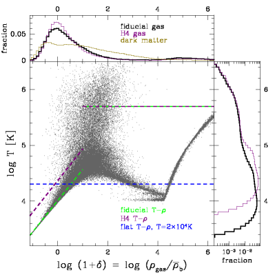
Figure 1: Distribution of particles in the temperature-overdensity plane for the fiducial simulation at z=2.4𝑧2.4z=2.4, with three imposed temperature-density relations over-plotted as labelled, as well as the temperature and overdensity distributions for the fiducial and H4 simulations. The hotter H4 gas is preferentially less dense than the lower pressure fiducial gas and pressureless dark matter.
Refer to caption
Figure 2: A 12.5×1×1h112.511superscript112.5\times 1\times 1\,h^{-1} Mpc comoving section of the fiducial simulation, in H I density, with 8<lognHI<08subscript𝑛HI0-8<\log n_{\mbox{\scriptsize{HI}}}<0 (note that the aspect ratio has not been preserved). The three green sightlines are separated by 100 h1superscript1h\,^{-1} kpc comoving; at z=2.4𝑧2.4z=2.4, corresponding to a projected separation of 4.94.94.9\arcsec.
Refer to caption
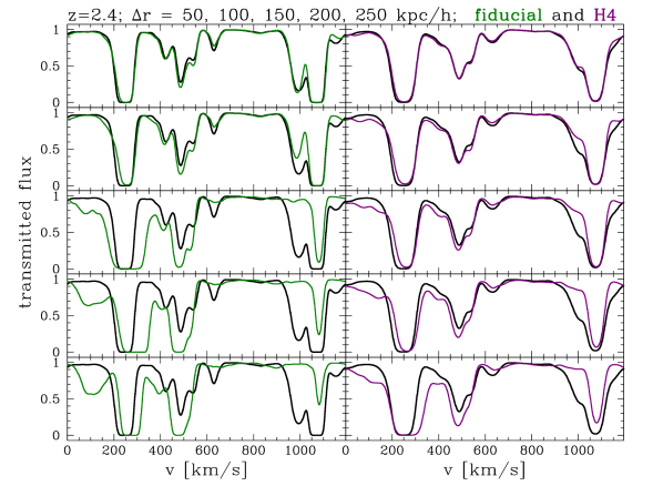
Figure 3: Sample paired lines of sight at z=2.4𝑧2.4z=2.4 separated by Δr=50Δ𝑟50\Delta r=50, 100, 150, 200, and 250 h1superscript1h^{-1} kpc comoving, from top to bottom, with the fiducial simulation on the left and the H4 simulation on the right. Within each column, the black spectra are the same (r=0𝑟0r=0). The top, middle, and bottom green spectra correspond to the three green sight lines in Fig. 2, with v=0𝑣0v=0 corresponding to the left-hand side of Fig. 2.

We use the same 2×28832superscript28832\times 288^{3} particle 12.5h112.5superscript112.5\,h^{-1} Mpc comoving smoothed particle hydrodynamic (SPH) simulations evolved with Gadget-2 (Springel, 2005) as in Paper I; hence we only present a basic description here. Throughout we adopt a ΛΛ\LambdaCDM cosmology of (Ωm,ΩΛ,Ωb,h,σ8,ns)=(0.25,0.75,0.044,0.7,0.8,0.95)subscriptΩ𝑚subscriptΩΛsubscriptΩ𝑏subscript𝜎8subscript𝑛𝑠0.250.750.0440.70.80.95(\Omega_{m},\Omega_{\Lambda},\Omega_{b},h,\sigma_{8},n_{s})=(0.25,0.75,0.044,0.7,0.8,0.95), which is in good agreement with the Wilkinson Microwave Anisotropy Probe 5-year results (Hinshaw et al., 2009). This cosmology leads to a gas particle mass of 1.426×10⁶M1.426superscript106subscriptMdirect-product1.426\times 10^{6}\,\mbox{M}_{\odot}, which is much less than the expected typical Jeans mass of 7×10⁹Msimilar-toabsent7superscript109subscriptMdirect-product\sim 7\times 10^{9}\,\mbox{M}_{\odot}. As a convergence test, we use a 2×14432superscript14432\times 144^{3} particle simulation that is otherwise identical to our fiducial simulation. The distribution of particles in the temperature-density plane for our “fiducial” simulation at z=3𝑧3z=3 is shown in Figure 1. The “H4” simulation has the same initial conditions as the fiducial one, but the heating rate from photoionization by the UV background is four times higher than in the fiducial simulation. An obvious consequence of this higher heating rate is that the H4 gas has higher temperatures than the fiducial gas. A more subtle effect, also shown in Figure 1, is that the hotter gas has a larger Jeans length and is hence smoother, with a smaller fraction of the gas at high overdensity. We therefore adopt three artificial temperature-density relations to isolate the effects of pressure support, thermal broadening, and the underlying overdensity distribution. As in Paper I, the fiducial and H4 temperature-density relations mimic the ones found in those simulations, while the flat T=2×10⁴𝑇2superscript104T=2\times 10^{4} K relation is used so that we can study the effects of thermally-broadened pressure support in the absence of overdensity-dependent thermal broadening. We impose these temperature-density relations on the fiducial and H4 gas distributions, as well as the fiducial dark matter, by assigning temperatures based solely on the local gas (or dark matter) overdensity, as demonstrated in Figure 1. For the fiducial and H4 relations, we set all gas with 1+δ101𝛿101+\delta\geq 10 to a “shocked” temperature T=5×10⁵𝑇5superscript105T=5\times 10^{5} K, while for the flat relation we set all the gas to T=2×10⁴𝑇2superscript104T=2\times 10^{4} K, regardless of density.

Table 1: Observed mean flux decrements D1eτdelimited-⟨⟩𝐷delimited-⟨⟩1superscript𝑒𝜏\langle D\rangle\equiv\langle 1-e^{-\tau}\rangle at z=2.4𝑧2.4z=2.4, 3, and 4 are from McDonald et al. (2000); the z=2𝑧2z=2 measurement is from Faucher-Giguère et al. (2008) without correcting for metal absorption. The observed temperature-density relations (T=T0[1+δ]α𝑇subscript𝑇0superscriptdelimited-[]1𝛿𝛼T=T_{0}[1+\delta]^{\alpha}) at z=2.4𝑧2.4z=2.4, 3, and 4 are from McDonald et al. (2001), with the z2similar-to𝑧2z\sim 2 measurement from Ricotti et al. (2000).
z𝑧z Ddelimited-⟨⟩𝐷\langle D\rangle observed T0subscript𝑇0T_{0} [K] observed α𝛼\alpha fiducial T0subscript𝑇0T_{0} [K] fiducial α𝛼\alpha H4 T0subscript𝑇0T_{0} [K] H4 α𝛼\alpha ΔθΔ𝜃\Delta\theta at
100h1100superscript1100\,h^{-1} kpc
4.0 0.525±0.012plus-or-minus0.5250.0120.525\pm 0.012 17400±3900plus-or-minus17400390017400\pm 3900 0.43±0.45plus-or-minus0.430.450.43\pm 0.45 117001170011700 0.540.540.54 28200 0.55 3.9″
3.0 0.316±0.023plus-or-minus0.3160.0230.316\pm 0.023 18300±1800plus-or-minus18300180018300\pm 1800 0.33±0.26plus-or-minus0.330.260.33\pm 0.26 110001100011000 0.570.570.57 25000 0.57 4.4″
or 18400±2100plus-or-minus18400210018400\pm 2100 0.29±0.30plus-or-minus0.290.300.29\pm 0.30
2.4 0.182±0.021plus-or-minus0.1820.0210.182\pm 0.021 17400±1900plus-or-minus17400190017400\pm 1900 0.52±0.14plus-or-minus0.520.140.52\pm 0.14 100001000010000 0.560.560.56 23000 0.57 4.9″
or 19200±2000plus-or-minus19200200019200\pm 2000 0.51±0.14plus-or-minus0.510.140.51\pm 0.14
2.0 0.144±0.024plus-or-minus0.1440.0240.144\pm 0.024 1770017700\quad 17700\quad\quad\quad 0.32±0.30plus-or-minus0.320.300.32\pm 0.30 891389138913 0.560.560.56 213802138021380 0.57 5.4″

At each redshift—z=2𝑧2z=2, 2.4, 3, and 4—we consider 200 lines of sight with paired sightlines separated by Δr=50Δ𝑟50\Delta r=50, 100, 125, 150, 175, 200, 250, 300, 400, and 500 h1superscript1h^{-1} kpc comoving for a total of 2200 sightlines per redshift for each of the overdensity–T𝑇T-ρ𝜌\rho combinations discussed above. In all cases we adjust the intensity of the UV background so that the mean flux decrement matches observational estimates (see Paper I for details). In Table 1, we list the adopted mean decrements and parameters for the observed, fiducial, and H4 temperature-density relations, as well as the projected angular separation at 100 h1superscript1h^{-1} kpc comoving.

3 Structure of the IGM & Transverse Lyα𝛼\alpha Coherence

To gain insight into the effects of temperature on the transverse coherence of the Lyα𝛼\alpha forest, we look at how paired sightlines differ in the fiducial and H4 simulations in § 3.1. We then quantify these differences by examining the relative changes in the flux decrement cross-correlation function in § 3.2 and the relative transverse coherence of the conditional flux decrement probability distribution in § 3.3.

3.1 Spectra

Before delving into statistical measures of the transverse Lyα𝛼\alpha forest, it will be instructive to first consider the underlying physical structures. In Figure 2, we show a small section of the fiducial simulation at z=2.4𝑧2.4z=2.4, where brighter regions correspond to higher H I densities. The observed transmitted flux is calculated as simply

F=eτLyα,𝐹superscript𝑒subscript𝜏Ly𝛼F=e^{-\tau_{{\rm Ly}\alpha}}, (5)

where τLyαsubscript𝜏Ly𝛼\tau_{{\rm Ly}\alpha} is the optical depth to Lyα𝛼\alpha photons. As discussed in detail in Paper I,

τLyαsubscript𝜏Ly𝛼\displaystyle\tau_{{\rm Ly}\alpha} proportional-to\displaystyle\propto nHIsubscript𝑛HI\displaystyle n_{\mbox{\tiny HI}}
proportional-to\displaystyle\propto (T0104K)0.7(1+δ)20.7α.superscriptsubscript𝑇0superscript104K0.7superscript1𝛿20.7𝛼\displaystyle\left(\frac{T_{0}}{10^{4}\,\mbox{K}}\right)^{-0.7}\left(1+\delta\right)^{2-0.7\alpha}.

The three sightlines in Figure 2 give rise to the top, middle, and bottom green spectra at z=2.4𝑧2.4z=2.4 in the left-hand panel of Figure 3. Figure 3 shows how pairs of spectra become more dissimilar as their transverse separation, ΔrΔ𝑟\Delta r, increases, and how this dissimilarity differs between the fiducial and H4 simulations. Spectral features remaining coherent over large scales correspond to physical structures that are parallel to the plane of the sky (see, e.g., the structures at 400<v<600400𝑣600400<v<600 km s-1), while spectral features disappearing from one sightline to the next correspond to physical structures that are more parallel to the line of sight (see, e.g., the features at v<300𝑣300v<300 km s-1). In general, the H4 spectra remain more similar than the fiducial ones as ΔrΔ𝑟\Delta r increases; we aim to determine to what extent this relatively higher coherence owes to pressure support rather than to the fact that the H4 spectra are individually inherently smoother because they have more thermal broadening than the fiducial spectra.

3.2 Cross-Correlation Functions

A common method for studying the transverse structure of the IGM is to look at the flux decrement cross-correlation function,

ξcrossD1(v)D2(v+Δv)D2,subscript𝜉crossdelimited-⟨⟩subscript𝐷1𝑣subscript𝐷2𝑣Δ𝑣superscriptdelimited-⟨⟩𝐷2\xi_{\rm cross}\equiv\frac{\langle D_{1}(v)D_{2}(v+\Delta v)\rangle}{\langle D\rangle^{2}}, (7)

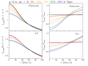
where D1F=1exp(τ)𝐷1𝐹1𝜏D\equiv 1-F=1-\exp(-\tau) and the two sightlines are separated by some ΔrΔ𝑟\Delta r (Miralda-Escudé et al., 1996; Rollinde et al., 2003). At Δr=0Δ𝑟0\Delta r=0, ξcrosssubscript𝜉cross\xi_{\rm cross} is just the auto-correlation function. The cross-correlation functions for the z=2.4𝑧2.4z=2.4 fiducial and H4 simulations at a range of ΔrΔ𝑟\Delta r are shown in the left-hand panels of Figure 4. At small ΔrΔ𝑟\Delta r and ΔvΔ𝑣\Delta v, the gas in the fiducial simulation has a higher ξcrosssubscript𝜉cross\xi_{\rm cross} than the gas in the H4 simulation because the smoother gas distribution has less rms density fluctuation. At larger ΔrΔ𝑟\Delta r and ΔvΔ𝑣\Delta v, the H4 gas has a higher ξcrosssubscript𝜉cross\xi_{\rm cross} owing to its greater coherence, as is visually evident in Figure 3. To quantify this relative change, ξcross/ξautosubscript𝜉crosssubscript𝜉auto\xi_{\rm cross}/\xi_{\rm auto} for the same selection of ΔrΔ𝑟\Delta r is plotted in the right-hand panels of Figure 4. Although in real space ξcross(Δr)=ξauto(HΔr)subscript𝜉crossΔ𝑟subscript𝜉auto𝐻Δ𝑟\xi_{\rm cross}(\Delta r)=\xi_{\rm auto}(H\Delta r), in velocity space redshift distortions preferentially suppress the auto-correlation function relative to the cross-correlation function, causing ξcross>ξautosubscript𝜉crosssubscript𝜉auto\xi_{\rm cross}>\xi_{\rm auto} for some regions of parameter space (McDonald & Miralda-Escudé, 1999; Marble et al., 2008b). The hotter, higher pressure, H4 simulation has a higher relative coherence (larger ξcross/ξautosubscript𝜉crosssubscript𝜉auto\xi_{\rm cross}/\xi_{\rm auto}) at small ΔvΔ𝑣\Delta v than the colder fiducial simulation.

Refer to caption
Figure 4: The cross-correlation function ξcrossD1(v)D2(v+Δv)/D2subscript𝜉crossdelimited-⟨⟩subscript𝐷1𝑣subscript𝐷2𝑣Δ𝑣superscriptdelimited-⟨⟩𝐷2\xi_{\rm cross}\equiv\langle D_{1}(v)D_{2}(v+\Delta v)\rangle/\langle D\rangle^{2} (left) and ξcross/ξautosubscript𝜉crosssubscript𝜉auto\xi_{\rm cross}/\xi_{\rm auto} (right) for the fiducial (top) and H4 (bottom) simulations for six different transverse separations Δr=50Δ𝑟50\Delta r=50, 100, 150, 200, and 250 h1superscript1h^{-1} kpc comoving. Note that the vertical scale in the left panels does not extend to 0.

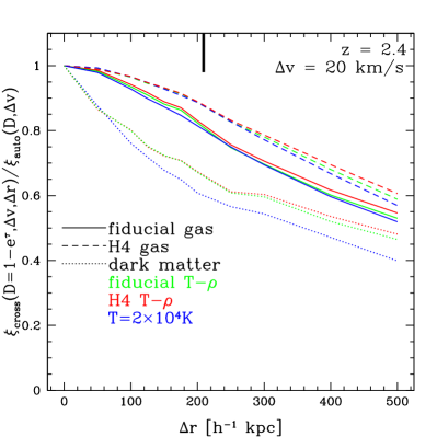
We compare a wider range of models in Figure 5, where we plot ξcross/ξautosubscript𝜉crosssubscript𝜉auto\xi_{\rm cross}/\xi_{\rm auto} as a function of ΔrΔ𝑟\Delta r at Δv=20Δ𝑣20\Delta v=20 km s-1 at z=2.4𝑧2.4z=2.4; this corresponds to taking a slice at Δv=20Δ𝑣20\Delta v=20 km s-1 in the right-hand panels of Figure 4. To elucidate whether the H4 gas is more strongly correlated because it has higher pressure, or because, as shown in detail in Paper I, hotter gas has more thermal broadening and therefore less small-scale structure, we also look at a range of T𝑇T-ρ𝜌\rho relations and overdensity fields. In this and in several of the following figures the line type (solid, dashed, or dotted) corresponds to the adopted overdensity field, either the gas overdensities from the fiducial simulation (solid lines), the gas overdensities from the H4 simulation (dashed lines) or the dark matter overdensities from the fiducial simulations. The line color corresponds to the adopted equation of state, i.e. the T𝑇T-ρ𝜌\rho relation, either the artificial fit to the relation from the fiducial simulation (green lines), the fit to the relation from the H4 simulation (red lines), or assuming a constant temperature of T=2×10⁴𝑇2superscript104T=2\times 10^{4} K (blue lines).

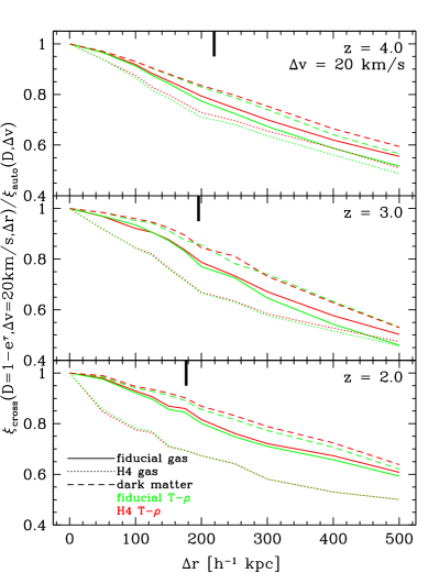
In Figure 5, the three choices for the overdensity field clearly separate into three distinct groups, with the highest-pressure H4 gas having the most transverse coherence and the zero-pressure dark matter having the least. Even non-thermally broadened spectra (which we have not plotted to avoid visual confusion) show the same relative decrease in coherence with increase in transverse separation as other spectra with the same underlying gas distributions. Within each overdensity group, ξcross/ξautosubscript𝜉crosssubscript𝜉auto\xi_{\rm cross}/\xi_{\rm auto} increases with increasing thermal broadening (e.g., the imposed H4 T𝑇T-ρ𝜌\rho relation yields higher ξcross/ξautosubscript𝜉crosssubscript𝜉auto\xi_{\rm cross}/\xi_{\rm auto} at all ΔrΔ𝑟\Delta r than imposing the fiducial T𝑇T-ρ𝜌\rho). However, lowering the resolution leads to offsets from the fiducial case by about the same amount as imposing different T𝑇T-ρ𝜌\rho relations. The same trends are seen at z=2𝑧2z=2, 3, and 4, as shown in Figure 6. In general, we find this delineation is clearer at 10Δv30less-than-or-similar-to10Δ𝑣less-than-or-similar-to3010\lesssim\Delta v\lesssim 30 km s-1 than at Δv=0Δ𝑣0\Delta v=0 or at larger velocity separations. The stark separation by overdensity distribution of the normalized cross-correlation function as a function of transverse separation is a clear sign that pressure plays an important role in the transverse structure of the Lyα𝛼\alpha forest.

Refer to caption
Figure 5: Normalized cross-correlation functions, ξcross/ξautosubscript𝜉crosssubscript𝜉auto\xi_{\rm cross}/\xi_{\rm auto}, as a function of the transverse separation ΔrΔ𝑟\Delta r for Δv=20Δ𝑣20\Delta v=20 km s-1 at z=2.4𝑧2.4z=2.4. The line type (solid, dashed, or dotted) denotes the adopted overdensity field and the line color the adopted T𝑇T-ρ𝜌\rho relation (see § 2 for details). The thick black tickmark denotes Δr=HΔvΔ𝑟𝐻Δ𝑣\Delta r=H\Delta v.
Refer to caption
Figure 6: Normalized cross-correlation functions, ξcross/ξautosubscript𝜉crosssubscript𝜉auto\xi_{\rm cross}/\xi_{\rm auto}, as a function of the transverse separation ΔrΔ𝑟\Delta r for Δv=20Δ𝑣20\Delta v=20 km s-1 at z=4𝑧4z=4, 3, and 2, from top to bottom. The models are denoted as in Fig. 5. The thick black tickmark denotes Δr=HΔvΔ𝑟𝐻Δ𝑣\Delta r=H\Delta v.

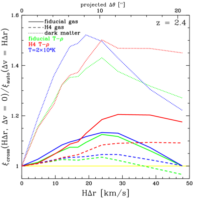
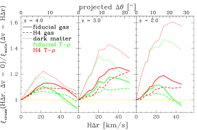
A common use for the flux decrement cross-correlation function is to measure the anisotropy in the Lyα𝛼\alpha forest caused by line-of-sight velocity distortions (Coppolani et al., 2006; D’Odorico et al., 2006), such as for the Alcock & Paczynski (1979) test (Hui et al., 1999; McDonald & Miralda-Escudé, 1999). In Figure 7, we compare ξcross(Δv=0,Δr)subscript𝜉crossΔ𝑣0Δ𝑟\xi_{\rm cross}(\Delta v=0,\Delta r) to the autocorrelation function at the same scale, ξauto(HΔr)subscript𝜉auto𝐻Δ𝑟\xi_{\rm auto}(H\Delta r), at z=2.4𝑧2.4z=2.4; higher values indicate higher levels of anisotropy. As in Figure 5, the models separate into groups of overdensity, and the differences between our low-resolution and fiducial cases are comparable with imposing different T𝑇T-ρ𝜌\rho relations on the fiducial gas. Figure 8 shows the same statistic for a smaller set of models at z=2𝑧2z=2, 3, and 4. As mentioned above, in real space ξcross(Δr)=ξauto(HΔr)subscript𝜉crossΔ𝑟subscript𝜉auto𝐻Δ𝑟\xi_{\rm cross}(\Delta r)=\xi_{\rm auto}(H\Delta r), but in (observed) velocity space, redshift distortions introduce anisotropy (Marble et al., 2008b). Because thermal broadening is an inherently one-dimensional anisotropic phenomenon, higher thermal broadening leads to higher anisotropy; we see this effect for each overdensity distribution in Figures 7 and 8. Pressure, on the other hand, is a three-dimensional inherently isotropic phenomenon: higher pressure therefore leads to less anisotropy, as we see from comparing the results for the dark matter, fiducial, and H4 overdensity fields. For HΔr20less-than-or-similar-to𝐻Δ𝑟20H\Delta r\lesssim 20 km s-1 (Δθ10less-than-or-similar-toΔ𝜃10\Delta\theta\lesssim 10\arcsec), the impact of thermal broadening on anisotropy is generally smaller than the impact of pressure.
Refer to caption
Figure 7: Normalized cross-correlation functions showing the anisotropy of the Lyα𝛼\alpha forest, ξcross/ξautosubscript𝜉crosssubscript𝜉auto\xi_{\rm cross}/\xi_{\rm auto}, as a function of Δv=HΔrΔ𝑣𝐻Δ𝑟\Delta v=H\Delta r, at z=2.4𝑧2.4z=2.4. The models are denoted as in Fig. 5
Refer to caption
Figure 8: Normalized cross-correlation functions showing the anisotropy of the Lyα𝛼\alpha forest, ξcross/ξautosubscript𝜉crosssubscript𝜉auto\xi_{\rm cross}/\xi_{\rm auto}, as a function of Δv=HΔrΔ𝑣𝐻Δ𝑟\Delta v=H\Delta r, at z=4𝑧4z=4, 3, and 2. The models are denoted as in Fig. 5

3.3 Conditional Flux Probability Distributions

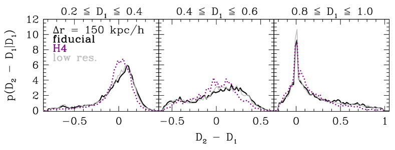
The structure of one-point flux probability distribution function (PDF) depends on both the thermal history and current thermal state of the gas, leading to a complex relationship between the effects of pressure support and thermal broadening on the PDF (Paper I). On the other hand, the interpretation of the conditional probability distribution function between paired sightlines (Miralda-Escudé et al., 1997) is relatively straightforward. For example, if for strongly absorbed pixels with 0.8D1<1.00.8subscript𝐷11.00.8\leq D_{1}<1.0, the pixels separated by ΔvΔ𝑣\Delta v on a sightline ΔrΔ𝑟\Delta r away are more strongly absorbed than randomly expected, then this might be a signature of strong transverse coherence and thus a large Jeans length. In Figure 9 we plot the flux decrement difference probability distributions, p(D2D1)𝑝subscript𝐷2subscript𝐷1p(D_{2}-D_{1}), for Δv=0Δ𝑣0\Delta v=0 and Δr=150h1Δ𝑟150superscript1\Delta r=150\,h^{-1} kpc and several bins of D1subscript𝐷1D_{1}, for the fiducial, H4, and low resolution gas at z=2.4𝑧2.4z=2.4. By looking at the PDF of the decrement differences, we can easily quantify the similarity of flux decrement pairs. The more strongly the distribution peaks around D2=D1subscript𝐷2subscript𝐷1D_{2}=D_{1}, the more coherent are the transverse structures. While the differences between the two simulations are not dramatic, the H4 model is consistently more strongly peaked around D2=D1subscript𝐷2subscript𝐷1D_{2}=D_{1}, with a stronger signature at low D1subscript𝐷1D_{1}. For most choices of D1subscript𝐷1D_{1}, this difference is much more pronounced than the difference between the fiducial and low-resolution simulations, indicating that our 2883superscript2883288^{3} particle simulations give robust results for this statistic.

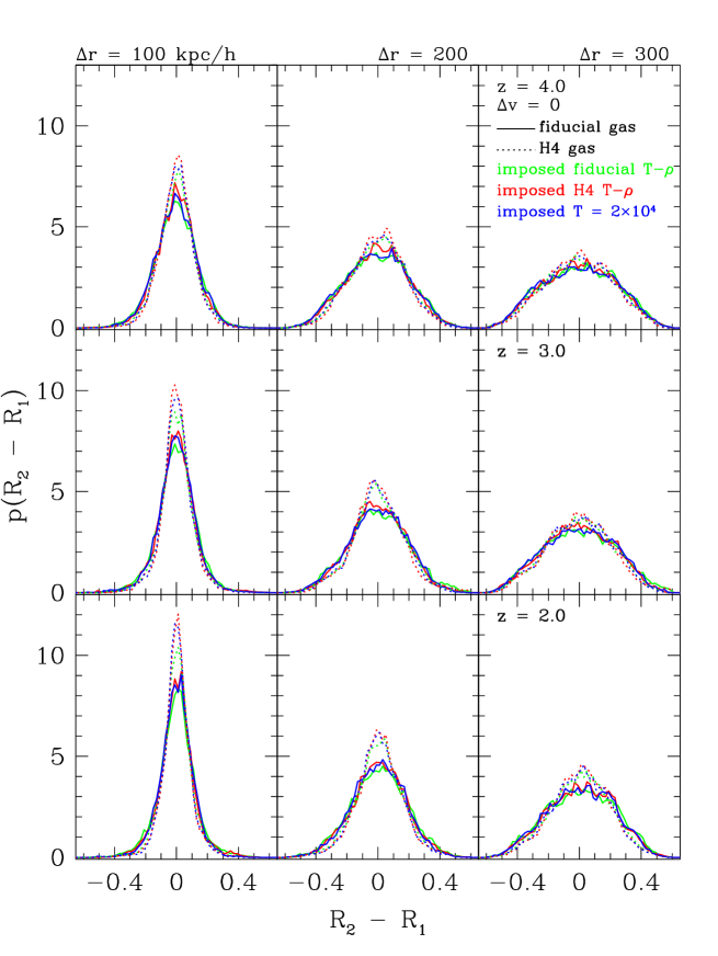
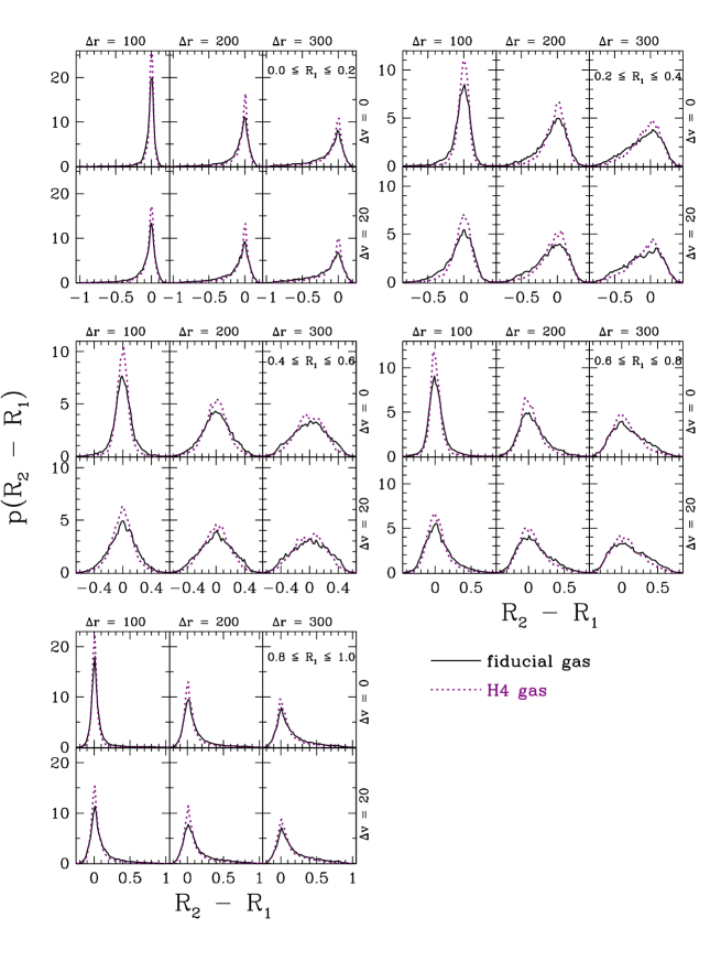
In Paper I we showed that the flux decrement PDFs for each of these T𝑇T-ρ𝜌\rho relations are fairly distinct, so some of the model differences in p(D2D1)𝑝subscript𝐷2subscript𝐷1p(D_{2}-D_{1}) could reflect differences in the underlying flux PDFs. We can remove this effect by converting from flux decrement D𝐷D to pixel rank Rp(<D)𝑅annotated𝑝absent𝐷R\equiv p(<D), the fraction of pixels with a flux decrement lower than D𝐷D. Of course, a fully successful model should reproduce the observed PDF, but here we wish to focus on transverse coherence and, therefore, remove any differences in the PDF caused by different temperature-density relations. Figure 10 shows that spectra generated from the H4 gas have rank difference distributions more strongly peaked around R2R1=0subscript𝑅2subscript𝑅10R_{2}-R_{1}=0 than spectra from the lower pressure, fiducial gas spectra. Changing the imposed temperature-density relation has less effect on the distributions than changing the underlying gas distribution, implying that (as expected) pressure rather than thermal broadening accounts for the larger transverse coherence. In general, the larger coherence appears at all redshifts, but it weakens with increasing ΔrΔ𝑟\Delta r. Non-thermally broadened spectra (not shown) have broader R2R1subscript𝑅2subscript𝑅1R_{2}-R_{1} distributions, so thermal broadening does play some role in transverse coherence. As with previous statistics, however, the lower resolution spectra differ from the fiducial case by about as much as spectra generated from different imposed T𝑇T-ρ𝜌\rho relations. Figure 11 presents the z=2.4𝑧2.4z=2.4 predictions in greater detail for the fiducial and H4 gas only, plotting five ranges of R1subscript𝑅1R_{1} and comparing Δv=0Δ𝑣0\Delta v=0 to Δv20similar-toΔ𝑣20\Delta v\sim 20 km s-1. The models are most easily distinguished at small ΔvΔ𝑣\Delta v and at small ΔrΔ𝑟\Delta r.

Refer to caption
Figure 9: Flux decrement difference probability distributions, p(D2D1)𝑝subscript𝐷2subscript𝐷1p(D_{2}-D_{1}) v. (D2D1)subscript𝐷2subscript𝐷1(D_{2}-D_{1}), at z=2.4𝑧2.4z=2.4, for Δv=0Δ𝑣0\Delta v=0 and Δr=150Δ𝑟150\Delta r=150. The three columns show D1[0.2,0.4)subscript𝐷10.20.4D_{1}\in[0.2,0.4) (left), D1[0.4,0.6)subscript𝐷10.40.6D_{1}\in[0.4,0.6) (middle), and D1[0.8,1.0]subscript𝐷10.81.0D_{1}\in[0.8,1.0] (right), with fiducial in black, H4 in purple (dotted), and the low resolution simulation in grey.
Refer to caption
Figure 10: Probability distributions for differences in flux decrement rank, p(R2R1)𝑝subscript𝑅2subscript𝑅1p(R_{2}-R_{1}) vs. (R2R1)subscript𝑅2subscript𝑅1(R_{2}-R_{1}) for Δv=0Δ𝑣0\Delta v=0, 0.4R10.60.4subscript𝑅10.60.4\leq R_{1}\leq 0.6, and z=4𝑧4z=4, 3, and 2.0 (top to bottom). The three columns show comoving transverse separations Δr=100Δ𝑟100\Delta r=100, 200, and 300 h1superscript1h^{-1} kpc (left to right). Regardless of the imposed temperature-density relation (indicated by line color), the H4 gas (dotted lines) is more strongly peaked around R2=R1subscript𝑅2subscript𝑅1R_{2}=R_{1} than the fiducial gas (solid lines) because the hotter gas has longer Jeans lengths and thus higher transverse coherence.
Refer to caption
Figure 11: Probability distributions for differences in flux decrement rank, p(R2R1)𝑝subscript𝑅2subscript𝑅1p(R_{2}-R_{1}) v. (R2R1)subscript𝑅2subscript𝑅1(R_{2}-R_{1}) for Δr=100Δ𝑟100\Delta r=100, 200, and 300 h1superscript1h^{-1} kpc comoving and Δv=0Δ𝑣0\Delta v=0 and 20 km s-1as labelled, for a range of R1subscript𝑅1R_{1} at z=2.4𝑧2.4z=2.4. The H4 gas (purple, dotted) is more strongly peaked around R2=R1subscript𝑅2subscript𝑅1R_{2}=R_{1} than the fiducial gas (black, solid) because the hotter gas has longer Jeans lengths and thus a higher transverse coherence.

In general, the slope of the temperature-density relation is much more difficult to observationally constrain than T0subscript𝑇0T_{0} because most methods for measuring the T𝑇T-ρ𝜌\rho relation are sensitive to only a limited range of τHIsubscript𝜏HI\tau_{\mbox{\tiny HI}} and hence 1+δ1𝛿1+\delta. Because (up to saturation) we can limit ourselves to a particular range of optical depth and thus 1+δ1𝛿1+\delta when using conditional rank distributions, it might be possible to use this technique to constrain the slope of the temperature-density relation. We cannot test this possibility using our current simulations because the fiducial and H4 temperature-density relations have similar slopes at all redshifts (see Table 1).

4 Conclusions

Recent efficient searches for binary quasars have yielded large samples of quasars with angular separations of 10less-than-or-similar-toabsent10\lesssim 10″ (Hennawi et al., 2006, 2009). The closely paired Lyman-α𝛼\alpha forest sightlines from such quasar pairs are ideal for studying the small-scale transverse structure of the intergalactic medium. We have shown using a set of smoothed particle hydrodynamic simulations with different equations of state that the coherence of transverse structure at these scales is determined primarily by the level of pressure support, i.e. the Jeans length, of the absorbing gas and is relatively insensitive to the amount of thermal broadening along the line of sight. Given the surprisingly high temperatures implied by single-sightline analyses (see discussions in §1 and Paper I), it would be valuable to investigate the thermal state of the IGM by this largely independent method.

Flux correlation functions (measured by, e.g., Rollinde et al. 2003; Coppolani et al. 2006; D’Odorico et al. 2006; Marble et al. 2008a) and the two-point distributions of flux decrements or pixel ranks can all be used to distinguish among gas distributions with different temperatures like the fiducial and H4 models considered here. Because the redshift ranges and pair separations will be dictated by the specifics of the available data sample, we provide in the form of electronic tables our simulated spectra along paired lines of sight from the two simulations, which can be used to generate predictions tailored to a particular data sample. These samples of spectra are described in §2 and the caption to Table 1. We caution that the finite size of our simulation volume could cause statistical fluctuations and systematic effects on our predictions, especially at large ΔrΔ𝑟\Delta r and ΔvΔ𝑣\Delta v; we will investigate this point in future work with larger simulations. The large increase in known quasar pairs, the ability of large telescopes to measure Lyman-α𝛼\alpha absorption spectra of relatively faint background sources, which have a high surface density on the sky, and the massive quasar sample expected from the Baryon Oscillation Spectroscopic Survey (Schlegel et al., 2009) will change the Lyα𝛼\alpha forest from a one-dimensional phenomenon to a three-dimensional phenomenon, opening new opportunities to constrain cosmology and the physics of the diffuse intergalactic medium.

Acknowledgments

We acknowledge a seminar by Joe Hennawi at the Ohio State Center for Cosmology and Astro-Particle Physics, which inspired this investigation; we also thank Joe Hennawi and Eduardo Rozo for helpful discussions and comments. We are grateful to the anonymous referee for thoughtful suggestions on the text. This work has been supported in part by NSF grant AST-0707985 and NASA ADP grant NNX08AJ44G.

References

  • Alcock & Paczynski (1979) Alcock, C. & Paczynski, B. 1979, Nature, 281, 358
  • Bechtold et al. (1994) Bechtold, J., Crotts, A. P. S., Duncan, R. C., & Fang, Y. 1994, ApJL, 437, L83
  • Bi & Davidsen (1997) Bi, H. & Davidsen, A. F. 1997, ApJ, 479, 523
  • Bolton et al. (2008) Bolton, J. S., Viel, M., Kim, T.-S., Haehnelt, M. G., & Carswell, R. F. 2008, MNRAS, 386, 1131
  • Cen et al. (1994) Cen, R., Miralda-Escudé, J., Ostriker, J. P., & Rauch, M. 1994, ApJL, 437, L9
  • Charlton et al. (1997) Charlton, J. C., Anninos, P., Zhang, Y., & Norman, M. L. 1997, ApJ, 485, 26
  • Coppolani et al. (2006) Coppolani, F., Petitjean, P., Stoehr, F., Rollinde, E., Pichon, C., Colombi, S., Haehnelt, M. G., Carswell, B., & Teyssier, R. 2006, MNRAS, 370, 1804
  • Crotts & Fang (1998) Crotts, A. P. S. & Fang, Y. 1998, ApJ, 502, 16
  • Desjacques & Nusser (2005) Desjacques, V. & Nusser, A. 2005, MNRAS, 361, 1257
  • Dinshaw et al. (1994) Dinshaw, N., Impey, C. D., Foltz, C. B., Weymann, R. J., & Chaffee, F. H. 1994, ApJL, 437, L87
  • D’Odorico et al. (1998) D’Odorico, V., Cristiani, S., D’Odorico, S., Fontana, A., Giallongo, E., & Shaver, P. 1998, A&A, 339, 678
  • D’Odorico et al. (2006) D’Odorico, V., Viel, M., Saitta, F., Cristiani, S., Bianchi, S., Boyle, B., Lopez, S., Maza, J., & Outram, P. 2006, MNRAS, 372, 1333
  • Fang et al. (1996) Fang, Y., Duncan, R. C., Crotts, A. P. S., & Bechtold, J. 1996, ApJ, 462, 77
  • Faucher-Giguère et al. (2008) Faucher-Giguère, C.-A., Prochaska, J. X., Lidz, A., Hernquist, L., & Zaldarriaga, M. 2008, ApJ, 681, 831
  • Gnedin & Hui (1998) Gnedin, N. Y. & Hui, L. 1998, MNRAS, 296, 44
  • Hennawi et al. (2009) Hennawi, J. F., Myers, A. D., Shen, Y., Strauss, M. A., Djorgovski, S. G., Fan, X., Glikman, E., Mahabal, A., Martin, C. L., Richards, G. T., Schneider, D. P., & Shankar, F. 2009, ArXiv:0908.3907
  • Hennawi et al. (2006) Hennawi, J. F., Strauss, M. A., Oguri, M., Inada, N., Richards, G. T., Pindor, B., Schneider, D. P., Becker, R. H., Gregg, M. D., Hall, P. B., Johnston, D. E., Fan, X., Burles, S., Schlegel, D. J., Gunn, J. E., Lupton, R. H., Bahcall, N. A., Brunner, R. J., & Brinkmann, J. 2006, AJ, 131, 1
  • Hernquist et al. (1996) Hernquist, L., Katz, N., Weinberg, D. H., & Miralda-Escudé, J. 1996, ApJL, 457, L51+
  • Hinshaw et al. (2009) Hinshaw, G., Weiland, J. L., Hill, R. S., Odegard, N., Larson, D., Bennett, C. L., Dunkley, J., Gold, B., Greason, M. R., Jarosik, N., Komatsu, E., Nolta, M. R., Page, L., Spergel, D. N., Wollack, E., Halpern, M., Kogut, A., Limon, M., Meyer, S. S., Tucker, G. S., & Wright, E. L. 2009, ApJS, 180, 225
  • Hui & Gnedin (1997) Hui, L. & Gnedin, N. Y. 1997, MNRAS, 292, 27
  • Hui et al. (1997) Hui, L., Gnedin, N. Y., & Zhang, Y. 1997, ApJ, 486, 599
  • Hui et al. (1999) Hui, L., Stebbins, A., & Burles, S. 1999, ApJL, 511, L5
  • Katz et al. (1996) Katz, N., Weinberg, D. H., & Hernquist, L. 1996, ApJS, 105, 19
  • Marble et al. (2008a) Marble, A. R., Eriksen, K. A., Impey, C. D., Bai, L., & Miller, L. 2008a, ApJS, 175, 29
  • Marble et al. (2008b) Marble, A. R., Eriksen, K. A., Impey, C. D., Oppenheimer, B. D., & Davé, R. 2008b, ApJ, 675, 946
  • McDonald & Miralda-Escudé (1999) McDonald, P. & Miralda-Escudé, J. 1999, ApJ, 518, 24
  • McDonald et al. (2001) McDonald, P., Miralda-Escudé, J., Rauch, M., Sargent, W. L. W., Barlow, T. A., & Cen, R. 2001, ApJ, 562, 52
  • McDonald et al. (2000) McDonald, P., Miralda-Escudé, J., Rauch, M., Sargent, W. L. W., Barlow, T. A., Cen, R., & Ostriker, J. P. 2000, ApJ, 543, 1
  • Miralda-Escudé et al. (1996) Miralda-Escudé, J., Cen, R., Ostriker, J. P., & Rauch, M. 1996, ApJ, 471, 582
  • Miralda-Escudé et al. (1997) Miralda-Escudé, J., Rauch, M., Sargent, W. L. W., Barlow, T. A., Weinberg, D. H., Hernquist, L., Katz, N., Cen, R., & Ostriker, J. P. 1997, in Structure and Evolution of the Intergalactic Medium from QSO Absorption Line System, ed. P. Petitjean & S. Charlot, 155–+
  • Rauch & Haehnelt (1995) Rauch, M. & Haehnelt, M. G. 1995, MNRAS, 275, L76
  • Reisenegger & Miralda-Escude (1995) Reisenegger, A. & Miralda-Escude, J. 1995, ApJ, 449, 476
  • Ricotti et al. (2000) Ricotti, M., Gnedin, N. Y., & Shull, J. M. 2000, ApJ, 534, 41
  • Rollinde et al. (2003) Rollinde, E., Petitjean, P., Pichon, C., Colombi, S., Aracil, B., D’Odorico, V., & Haehnelt, M. G. 2003, MNRAS, 341, 1279
  • Schaye (2001) Schaye, J. 2001, ApJ, 559, 507
  • Schaye et al. (2000) Schaye, J., Theuns, T., Rauch, M., Efstathiou, G., & Sargent, W. L. W. 2000, MNRAS, 318, 817
  • Schlegel et al. (2009) Schlegel, D., White, M., & Eisenstein, D. 2009, in Astronomy, Vol. 2010, AGB Stars and Related Phenomenastro2010: The Astronomy and Astrophysics Decadal Survey, 314–+
  • Schneider et al. (2006) Schneider, P., Kochanek, C. S., & Wambsganss, J. 2006, Gravitational Lensing: Strong, Weak and Micro (Gravitational Lensing: Strong, Weak and Micro: , Saas-Fee Advanced Courses, Volume 33. ISBN 978-3-540-30309-1. Springer-Verlag Berlin Heidelberg, 2006)
  • Springel (2005) Springel, V. 2005, MNRAS, 364, 1105
  • Theuns et al. (2002) Theuns, T., Schaye, J., Zaroubi, S., Kim, T.-S., Tzanavaris, P., & Carswell, B. 2002, ApJL, 567, L103
  • Viel et al. (2002) Viel, M., Matarrese, S., Mo, H. J., Haehnelt, M. G., & Theuns, T. 2002, MNRAS, 329, 848
  • Zhang et al. (1995) Zhang, Y., Anninos, P., & Norman, M. L. 1995, ApJL, 453, L57+

Appendix A Format of associated electronic tables

We provide in the form of electronic tables our simulated spectra, the H I optical depth as a function of velocity and transverse separation, along paired sightlines from the fiducial and H4 simulations at z=2𝑧2z=2, 2.4, 3, and 4. We show in Table LABEL:tab:spec a portion of the spectra from the fiducial simulation at z=2𝑧2z=2.

Table 2: Sample paired spectra for the fiducial simulation at z=2𝑧2z=2. Each set of 1250 lines corresponds to an independent sightline and its pairs. This table is published in their entirety online; a portion is shown here for guidance regarding its form and content.
τHIsubscript𝜏HI\tau_{\rm HI} at transverse separation ΔrΔ𝑟\Delta r in h1superscript1h^{-1} kpc comoving
v𝑣v [ km s-1] 00 505050 100100100 125125125 150150150 175175175 200200200 250250250 300300300 400400400 500500500
0.4564350.4564350.456435 0.03312190.03312190.0331219 0.02850250.02850250.0285025 0.02889730.02889730.0288973 0.02974250.02974250.0297425 0.03038960.03038960.0303896 0.03086830.03086830.0308683 0.03164290.03164290.0316429 0.03717950.03717950.0371795 0.04693230.04693230.0469323 0.05217550.05217550.0521755 0.04741180.04741180.0474118
1.36931.36931.3693 0.03148170.03148170.0314817 0.02745380.02745380.0274538 0.02802370.02802370.0280237 0.02893960.02893960.0289396 0.02966750.02966750.0296675 0.03024560.03024560.0302456 0.03111120.03111120.0311112 0.03674470.03674470.0367447 0.04628020.04628020.0462802 0.05112940.05112940.0511294 0.04593190.04593190.0459319
2.282172.282172.28217 0.03012460.03012460.0301246 0.02657710.02657710.0265771 0.02725630.02725630.0272563 0.02821590.02821590.0282159 0.02901170.02901170.0290117 0.02968890.02968890.0296889 0.03065510.03065510.0306551 0.03641660.03641660.0364166 0.04577520.04577520.0457752 0.05026360.05026360.0502636 0.04464470.04464470.0446447
3.195043.195043.19504 0.02900660.02900660.0290066 0.02584010.02584010.0258401 0.02657730.02657730.0265773 0.02756090.02756090.0275609 0.0284160.0284160.028416 0.02919310.02919310.0291931 0.03026790.03026790.0302679 0.03618350.03618350.0361835 0.04540740.04540740.0454074 0.04956660.04956660.0495666 0.04354580.04354580.0435458
4.10794.10794.1079 0.0280880.0280880.028088 0.02521510.02521510.0252151 0.02597220.02597220.0259722 0.02696650.02696650.0269665 0.02787590.02787590.0278759 0.02875380.02875380.0287538 0.02994330.02994330.0299433 0.03603410.03603410.0360341 0.04516570.04516570.0451657 0.0490250.0490250.049025 0.04262950.04262950.0426295
5.020775.020775.02077 0.02733320.02733320.0273332 0.02467890.02467890.0246789 0.02542910.02542910.0254291 0.0264260.0264260.026426 0.02738760.02738760.0273876 0.02836710.02836710.0283671 0.02967580.02967580.0296758 0.03595810.03595810.0359581 0.04503780.04503780.0450378 0.04862380.04862380.0486238 0.0418890.0418890.041889
5.933645.933645.93364 0.02671170.02671170.0267117 0.02421270.02421270.0242127 0.02493880.02493880.0249388 0.02593460.02593460.0259346 0.0269480.0269480.026948 0.02802960.02802960.0280296 0.02946030.02946030.0294603 0.03594560.03594560.0359456 0.04501030.04501030.0450103 0.04834730.04834730.0483473 0.04131570.04131570.0413157
6.84656.84656.8465 0.02619780.02619780.0261978 0.02380130.02380130.0238013 0.02449380.02449380.0244938 0.02548820.02548820.0254882 0.02655480.02655480.0265548 0.02773830.02773830.0277383 0.02929240.02929240.0292924 0.03598740.03598740.0359874 0.04506880.04506880.0450688 0.04817950.04817950.0481795 0.04089990.04089990.0408999
7.759377.759377.75937 0.02577040.02577040.0257704 0.02343290.02343290.0234329 0.02408840.02408840.0240884 0.02508380.02508380.0250838 0.02620580.02620580.0262058 0.02749060.02749060.0274906 0.02916830.02916830.0291683 0.03607490.03607490.0360749 0.04519850.04519850.0451985 0.04810450.04810450.0481045 0.04063080.04063080.0406308
8.672248.672248.67224 0.02541270.02541270.0254127 0.02309880.02309880.0230988 0.02371790.02371790.0237179 0.0247190.0247190.024719 0.0258990.0258990.025899 0.02728410.02728410.0272841 0.02908470.02908470.0290847 0.03619980.03619980.0361998 0.04538390.04538390.0453839 0.04810740.04810740.0481074 0.04049720.04049720.0404972
1139.711139.711139.71 0.03743950.03743950.0374395 0.03126890.03126890.0312689 0.0310530.0310530.031053 0.0316420.0316420.031642 0.03206510.03206510.0320651 0.03233690.03233690.0323369 0.0329630.0329630.032963 0.03841910.03841910.0384191 0.04870980.04870980.0487098 0.05484280.05484280.0548428 0.05096720.05096720.0509672
1140.631140.631140.63 0.03509170.03509170.0350917 0.02976040.02976040.0297604 0.02989850.02989850.0298985 0.03063790.03063790.0306379 0.03118560.03118560.0311856 0.03156310.03156310.0315631 0.03225760.03225760.0322576 0.03773330.03773330.0377333 0.04773980.04773980.0477398 0.05341110.05341110.0534111 0.04908870.04908870.0490887
0.4564350.4564350.456435 0.00972110.00972110.0097211 0.00874740.00874740.0087474 0.008503570.008503570.00850357 0.008699640.008699640.00869964 0.00875970.00875970.0087597 0.008845410.008845410.00884541 0.009295910.009295910.00929591 0.01029070.01029070.0102907 0.010990.010990.01099 0.01100820.01100820.0110082 0.009801520.009801520.00980152
1.36931.36931.3693 0.01023720.01023720.0102372 0.009209840.009209840.00920984 0.009015550.009015550.00901555 0.009286030.009286030.00928603 0.009387220.009387220.00938722 0.009509450.009509450.00950945 0.01004690.01004690.0100469 0.01116180.01116180.0111618 0.01185160.01185160.0118516 0.01173590.01173590.0117359 0.01031040.01031040.0103104
Table 3: Same as Table 2 but for the H4 simulation at z=2𝑧2z=2.
τHIsubscript𝜏HI\tau_{\rm HI} at transverse separation ΔrΔ𝑟\Delta r in h1superscript1h^{-1} kpc comoving
v𝑣v [ km s-1] 00 505050 100100100 125125125 150150150 175175175 200200200 250250250 300300300 400400400 500500500
0.4564350.4564350.456435 0.07487270.07487270.0748727 0.05940090.05940090.0594009 0.05344430.05344430.0534443 0.0526530.0526530.052653 0.05235010.05235010.0523501 0.05186540.05186540.0518654 0.05004430.05004430.0500443 0.04881910.04881910.0488191 0.0506990.0506990.050699 0.06848180.06848180.0684818 0.1144940.1144940.114494
1.36931.36931.3693 0.07246160.07246160.0724616 0.05688170.05688170.0568817 0.05101250.05101250.0510125 0.05019110.05019110.0501911 0.0498560.0498560.049856 0.04948140.04948140.0494814 0.04781770.04781770.0478177 0.04683760.04683760.0468376 0.04857930.04857930.0485793 0.06598980.06598980.0659898 0.1116610.1116610.111661
2.282172.282172.28217 0.0700310.0700310.070031 0.05443530.05443530.0544353 0.04868470.04868470.0486847 0.04785250.04785250.0478525 0.04750570.04750570.0475057 0.04725240.04725240.0472524 0.04575020.04575020.0457502 0.04501430.04501430.0450143 0.04663290.04663290.0466329 0.06370980.06370980.0637098 0.1089380.1089380.108938
1139.711139.711139.71 0.07958990.07958990.0795899 0.06461170.06461170.0646117 0.05857120.05857120.0585712 0.05789970.05789970.0578997 0.05772960.05772960.0577296 0.05707070.05707070.0570707 0.05496190.05496190.0549619 0.05326150.05326150.0532615 0.05546790.05546790.0554679 0.07410660.07410660.0741066 0.1205190.1205190.120519
1140.631140.631140.63 0.07725250.07725250.0772525 0.06198160.06198160.0619816 0.05596830.05596830.0559683 0.05522690.05522690.0552269 0.05497860.05497860.0549786 0.0543980.0543980.054398 0.05242730.05242730.0524273 0.05096050.05096050.0509605 0.05299490.05299490.0529949 0.07118760.07118760.0711876 0.1174450.1174450.117445
0.4564350.4564350.456435 0.01563310.01563310.0156331 0.01604740.01604740.0160474 0.01639630.01639630.0163963 0.01636150.01636150.0163615 0.01587820.01587820.0158782 0.0154660.0154660.015466 0.01527690.01527690.0152769 0.01419060.01419060.0141906 0.01365510.01365510.0136551 0.01219230.01219230.0121923 0.01120080.01120080.0112008
Table 4: Same as Table 2 but for the fiducial simulation at z=2.4𝑧2.4z=2.4.
τHIsubscript𝜏HI\tau_{\rm HI} at transverse separation ΔrΔ𝑟\Delta r in h1superscript1h^{-1} kpc comoving
v𝑣v [ km s-1] 00 505050 100100100 125125125 150150150 175175175 200200200 250250250 300300300 400400400 500500500
0.4782460.4782460.478246 0.01994920.01994920.0199492 0.01870340.01870340.0187034 0.01637450.01637450.0163745 0.01543530.01543530.0154353 0.01440060.01440060.0144006 0.01320770.01320770.0132077 0.01223550.01223550.0122355 0.01164670.01164670.0116467 0.01392850.01392850.0139285 0.02371590.02371590.0237159 0.04374920.04374920.0437492
1.434741.434741.43474 0.02011310.02011310.0201131 0.01876720.01876720.0187672 0.01633320.01633320.0163332 0.01537070.01537070.0153707 0.01430520.01430520.0143052 0.01306110.01306110.0130611 0.01205480.01205480.0120548 0.01142720.01142720.0114272 0.01369590.01369590.0136959 0.02372120.02372120.0237212 0.04497790.04497790.0449779
2.391232.391232.39123 0.02028820.02028820.0202882 0.01884740.01884740.0188474 0.01630760.01630760.0163076 0.01532040.01532040.0153204 0.01422590.01422590.0142259 0.01292650.01292650.0129265 0.01188480.01188480.0118848 0.01121290.01121290.0112129 0.01346180.01346180.0134618 0.02371920.02371920.0237192 0.04624620.04624620.0462462
1194.181194.181194.18 0.01966090.01966090.0196609 0.01863090.01863090.0186309 0.01650930.01650930.0165093 0.01561270.01561270.0156127 0.01463950.01463950.0146395 0.01353990.01353990.0135399 0.01262930.01262930.0126293 0.01209780.01209780.0120978 0.01438270.01438270.0143827 0.02368180.02368180.0236818 0.04140310.04140310.0414031
1195.141195.141195.14 0.01979780.01979780.0197978 0.01865730.01865730.0186573 0.01643280.01643280.0164328 0.01551570.01551570.0155157 0.0145120.0145120.014512 0.01336730.01336730.0133673 0.01242720.01242720.0124272 0.01187060.01187060.0118706 0.01415790.01415790.0141579 0.02370280.02370280.0237028 0.04255820.04255820.0425582
0.4782460.4782460.478246 0.1922980.1922980.192298 0.1003750.1003750.100375 0.069540.069540.06954 0.07238890.07238890.0723889 0.08008620.08008620.0800862 0.08907430.08907430.0890743 0.1002840.1002840.100284 0.1303560.1303560.130356 0.1652080.1652080.165208 0.1336480.1336480.133648 0.08578220.08578220.0857822
Table 5: Same as Table 2 but for the H4 simulation at z=2.4𝑧2.4z=2.4.
τHIsubscript𝜏HI\tau_{\rm HI} at transverse separation ΔrΔ𝑟\Delta r in h1superscript1h^{-1} kpc comoving
v𝑣v [ km s-1] 00 505050 100100100 125125125 150150150 175175175 200200200 250250250 300300300 400400400 500500500
0.4782460.4782460.478246 0.01630390.01630390.0163039 0.01548590.01548590.0154859 0.01488150.01488150.0148815 0.01518270.01518270.0151827 0.01588830.01588830.0158883 0.01671970.01671970.0167197 0.01790850.01790850.0179085 0.01930290.01930290.0193029 0.01893210.01893210.0189321 0.02096390.02096390.0209639 0.03990290.03990290.0399029
1.434741.434741.43474 0.01629740.01629740.0162974 0.01545430.01545430.0154543 0.01479490.01479490.0147949 0.01511150.01511150.0151115 0.01584180.01584180.0158418 0.01670080.01670080.0167008 0.0179510.0179510.017951 0.01945450.01945450.0194545 0.01911340.01911340.0191134 0.02137790.02137790.0213779 0.04046020.04046020.0404602
2.391232.391232.39123 0.01632070.01632070.0163207 0.0154480.0154480.015448 0.01472610.01472610.0147261 0.01505770.01505770.0150577 0.01581050.01581050.0158105 0.01669310.01669310.0166931 0.01800170.01800170.0180017 0.019610.019610.01961 0.01930010.01930010.0193001 0.02182020.02182020.0218202 0.0410280.0410280.041028
1194.181194.181194.18 0.01640180.01640180.0164018 0.01562070.01562070.0156207 0.0151070.0151070.015107 0.01537660.01537660.0153766 0.0160260.0160260.016026 0.01679010.01679010.0167901 0.01784720.01784720.0178472 0.01901160.01901160.0190116 0.01858410.01858410.0185841 0.02021350.02021350.0202135 0.03882430.03882430.0388243
1195.141195.141195.14 0.01633910.01633910.0163391 0.01554170.01554170.0155417 0.01498560.01498560.0149856 0.01527110.01527110.0152711 0.01594980.01594980.0159498 0.01674950.01674950.0167495 0.01787390.01787390.0178739 0.01915520.01915520.0191552 0.01875570.01875570.0187557 0.02057640.02057640.0205764 0.03935730.03935730.0393573
0.4782460.4782460.478246 0.2109830.2109830.210983 0.2302440.2302440.230244 0.2437470.2437470.243747 0.2225630.2225630.222563 0.1924810.1924810.192481 0.1686560.1686560.168656 0.146490.146490.14649 0.126040.126040.12604 0.1229420.1229420.122942 0.1166940.1166940.116694 0.1348030.1348030.134803
Table 6: Same as Table 2 but for the fiducial simulation at z=3𝑧3z=3.
τHIsubscript𝜏HI\tau_{\rm HI} at transverse separation ΔrΔ𝑟\Delta r in h1superscript1h^{-1} kpc comoving
v𝑣v [ km s-1] 00 505050 100100100 125125125 150150150 175175175 200200200 250250250 300300300 400400400 500500500
0.5115840.5115840.511584 2.81162.81162.8116 2.658212.658212.65821 1.901551.901551.90155 1.564011.564011.56401 1.2461.2461.246 1.011551.011551.01155 0.7797780.7797780.779778 0.5346220.5346220.534622 0.4512760.4512760.451276 0.4416480.4416480.441648 0.5798920.5798920.579892
1.534751.534751.53475 2.812122.812122.81212 2.63162.63162.6316 1.86721.86721.8672 1.530381.530381.53038 1.219461.219461.21946 0.9959490.9959490.995949 0.7733770.7733770.773377 0.5342130.5342130.534213 0.4535970.4535970.453597 0.44460.44460.4446 0.5773580.5773580.577358
2.557922.557922.55792 2.808932.808932.80893 2.597792.597792.59779 1.828051.828051.82805 1.492171.492171.49217 1.189091.189091.18909 0.977370.977370.97737 0.7653170.7653170.765317 0.5338750.5338750.533875 0.4566410.4566410.456641 0.4484730.4484730.448473 0.5746690.5746690.574669
1277.431277.431277.43 2.79892.79892.7989 2.689872.689872.68987 1.95591.95591.9559 1.617381.617381.61738 1.287481.287481.28748 1.033881.033881.03388 0.7877560.7877560.787756 0.5358210.5358210.535821 0.4495410.4495410.449541 0.4391440.4391440.439144 0.5847460.5847460.584746
1278.451278.451278.45 2.807222.807222.80722 2.67762.67762.6776 1.931091.931091.93109 1.592991.592991.59299 1.268641.268641.26864 1.024161.024161.02416 0.7845390.7845390.784539 0.535150.535150.53515 0.4498830.4498830.449883 0.4398050.4398050.439805 0.5823380.5823380.582338
0.5115840.5115840.511584 0.1760820.1760820.176082 0.1678290.1678290.167829 0.1212780.1212780.121278 0.1261080.1261080.126108 0.105530.105530.10553 0.09091430.09091430.0909143 0.1516230.1516230.151623 0.07662370.07662370.0766237 0.1725810.1725810.172581 0.2996470.2996470.299647 0.5347140.5347140.534714
Table 7: Same as Table 2 but for the H4 simulation at z=3𝑧3z=3.
τHIsubscript𝜏HI\tau_{\rm HI} at transverse separation ΔrΔ𝑟\Delta r in h1superscript1h^{-1} kpc comoving
v𝑣v [ km s-1] 00 505050 100100100 125125125 150150150 175175175 200200200 250250250 300300300 400400400 500500500
0.5115840.5115840.511584 1.347651.347651.34765 1.251071.251071.25107 1.100451.100451.10045 1.019871.019871.01987 0.9541730.9541730.954173 0.8512630.8512630.851263 0.7897650.7897650.789765 0.6207370.6207370.620737 0.4563760.4563760.456376 0.3999120.3999120.399912 0.7384520.7384520.738452
1.534751.534751.53475 1.372281.372281.37228 1.254371.254371.25437 1.094551.094551.09455 1.008681.008681.00868 0.9401730.9401730.940173 0.8361380.8361380.836138 0.7732570.7732570.773257 0.6069030.6069030.606903 0.4454880.4454880.445488 0.3966620.3966620.396662 0.7520270.7520270.752027
2.557922.557922.55792 1.399851.399851.39985 1.259411.259411.25941 1.089581.089581.08958 0.9984280.9984280.998428 0.9269760.9269760.926976 0.821690.821690.82169 0.7572780.7572780.757278 0.5932450.5932450.593245 0.434610.434610.43461 0.3930980.3930980.393098 0.7650660.7650660.765066
1277.431277.431277.43 1.306631.306631.30663 1.249651.249651.24965 1.115381.115381.11538 1.045341.045341.04534 0.9847990.9847990.984799 0.8836270.8836270.883627 0.8243780.8243780.824378 0.6489410.6489410.648941 0.4780360.4780360.478036 0.4055210.4055210.405521 0.7100040.7100040.710004
1278.451278.451278.45 1.325811.325811.32581 1.249491.249491.24949 1.107371.107371.10737 1.032061.032061.03206 0.9690320.9690320.969032 0.8670870.8670870.867087 0.8068070.8068070.806807 0.6347490.6347490.634749 0.4672370.4672370.467237 0.4028570.4028570.402857 0.7244170.7244170.724417
0.5115840.5115840.511584 0.236950.236950.23695 0.1829670.1829670.182967 0.1465730.1465730.146573 0.1533920.1533920.153392 0.1380040.1380040.138004 0.1263270.1263270.126327 0.1770610.1770610.177061 0.09888520.09888520.0988852 0.2640860.2640860.264086 0.3507530.3507530.350753 0.3993630.3993630.399363
Table 8: Same as Table 2 but for the fiducial simulation at z=4𝑧4z=4.
τHIsubscript𝜏HI\tau_{\rm HI} at transverse separation ΔrΔ𝑟\Delta r in h1superscript1h^{-1} kpc comoving
v𝑣v [ km s-1] 00 505050 100100100 125125125 150150150 175175175 200200200 250250250 300300300 400400400 500500500
0.5656850.5656850.565685 0.6610790.6610790.661079 0.5050360.5050360.505036 0.4161280.4161280.416128 0.394170.394170.39417 0.3935080.3935080.393508 0.4005540.4005540.400554 0.4112890.4112890.411289 0.4383010.4383010.438301 0.3814880.3814880.381488 0.2858830.2858830.285883 0.2352780.2352780.235278
1.697051.697051.69705 0.669840.669840.66984 0.5134740.5134740.513474 0.424430.424430.42443 0.4024050.4024050.402405 0.4009140.4009140.400914 0.4061960.4061960.406196 0.415160.415160.41516 0.4392560.4392560.439256 0.362920.362920.36292 0.2729590.2729590.272959 0.2259430.2259430.225943
2.828432.828432.82843 0.6781330.6781330.678133 0.5216620.5216620.521662 0.4323520.4323520.432352 0.4103540.4103540.410354 0.408010.408010.40801 0.411440.411440.41144 0.4185320.4185320.418532 0.4397550.4397550.439755 0.3449360.3449360.344936 0.2609420.2609420.260942 0.2175930.2175930.217593
1412.521412.521412.52 0.6425510.6425510.642551 0.4878530.4878530.487853 0.3989490.3989490.398949 0.3773280.3773280.377328 0.3781220.3781220.378122 0.3882810.3882810.388281 0.402120.402120.40212 0.4347160.4347160.434716 0.4201450.4201450.420145 0.3144310.3144310.314431 0.2573420.2573420.257342
1413.651413.651413.65 0.6519410.6519410.651941 0.4964580.4964580.496458 0.4075880.4075880.407588 0.3857720.3857720.385772 0.3858810.3858810.385881 0.3945650.3945650.394565 0.4069350.4069350.406935 0.4368120.4368120.436812 0.400580.400580.40058 0.2997120.2997120.299712 0.2457070.2457070.245707
0.5656850.5656850.565685 1.145911.145911.14591 0.6854820.6854820.685482 0.4573770.4573770.457377 0.3973350.3973350.397335 0.3802560.3802560.380256 0.3290110.3290110.329011 0.2897360.2897360.289736 0.2406640.2406640.240664 0.1964830.1964830.196483 0.1651880.1651880.165188 0.2097430.2097430.209743
Table 9: Same as Table 2 but for the H4 simulation at z=4𝑧4z=4.
τHIsubscript𝜏HI\tau_{\rm HI} at transverse separation ΔrΔ𝑟\Delta r in h1superscript1h^{-1} kpc comoving
v𝑣v [ km s-1] 00 505050 100100100 125125125 150150150 175175175 200200200 250250250 300300300 400400400 500500500
0.5656850.5656850.565685 0.46770.46770.4677 0.4558040.4558040.455804 0.4099490.4099490.409949 0.3771380.3771380.377138 0.3475360.3475360.347536 0.3266760.3266760.326676 0.3122840.3122840.312284 0.3011440.3011440.301144 0.3754850.3754850.375485 0.4305070.4305070.430507 0.4512280.4512280.451228
1.697051.697051.69705 0.4644390.4644390.464439 0.4526060.4526060.452606 0.4069870.4069870.406987 0.3743290.3743290.374329 0.3445160.3445160.344516 0.3233490.3233490.323349 0.3090210.3090210.309021 0.2991820.2991820.299182 0.3649590.3649590.364959 0.4136160.4136160.413616 0.4348750.4348750.434875
2.828432.828432.82843 0.4613090.4613090.461309 0.4494340.4494340.449434 0.4038650.4038650.403865 0.3713050.3713050.371305 0.3412510.3412510.341251 0.3197630.3197630.319763 0.3054910.3054910.305491 0.2969450.2969450.296945 0.3547580.3547580.354758 0.397290.397290.39729 0.4188320.4188320.418832
1412.521412.521412.52 0.4742080.4742080.474208 0.4619190.4619190.461919 0.415170.415170.41517 0.3819260.3819260.381926 0.3526580.3526580.352658 0.3323830.3323830.332383 0.3178550.3178550.317855 0.3041620.3041620.304162 0.3974790.3974790.397479 0.4660410.4660410.466041 0.4848750.4848750.484875
1413.651413.651413.65 0.4709930.4709930.470993 0.4589390.4589390.458939 0.4126950.4126950.412695 0.3796850.3796850.379685 0.3502630.3502630.350263 0.3297010.3297010.329701 0.3152410.3152410.315241 0.302810.302810.30281 0.3863270.3863270.386327 0.4479770.4479770.447977 0.4678940.4678940.467894
0.5656850.5656850.565685 1.925881.925881.92588 1.134131.134131.13413 0.6553670.6553670.655367 0.5802320.5802320.580232 0.5461410.5461410.546141 0.5217370.5217370.521737 0.4759620.4759620.475962 0.3632750.3632750.363275 0.2988740.2988740.298874 0.2600410.2600410.260041 0.2148790.2148790.214879