Compressed Blind De-convolution of Filtered Sparse Processes††thanks: This research was supported by NSF CAREER award ECS 0449194
Abstract
Suppose the signal is realized by driving a k-sparse signal through an arbitrary unknown stable discrete-linear time invariant system , namely, , where is the impulse response of the operator . Is compressible in the conventional sense of compressed sensing? Namely, can be reconstructed from small set of measurements obtained through suitable random projections? For the case when the unknown system is auto-regressive (i.e. all pole) of a known order it turns out that can indeed be reconstructed from measurements. We develop a novel LP optimization algorithm and show that both the unknown filter and the sparse input can be reliably estimated.
1 Introduction
In this paper we focus on blind de-convolution problems for filtered sparse processes. These types of processes naturally arise in reflection seismology [1]. The LTI system is commonly referred to as the wavelet, which can be unknown, and serves as the input signal. This input signal passes through the different layers of earth and the reflected signal corresponds to the reflection coefficients from the different layers. The signal is typically sparse. The reflected output, which is referred to as the seismic trace, is recorded by a geophone. Other applications of filtered sparse processes include nuclear radiation [2], neuronal spike trains [3] and communications [4].
Specifically, a sparse input is filtered by an unknown infinite impulse response (IIR) discrete time stable linear filter and the resulting output
is measured in Gaussian noise, namely, for . The goal is to detect , and estimate the filter . The main approach heretofore proposed for blind de-convolution involves heuristic iterative block decomposition schemes (first proposed in [5]). Here the filter and sparse inputs are alternatively estimated by holding one of them constant. While these algorithms can work in some cases, no systematic performance guarantees currently exist. We explore a convex optimization framework for blind de-convolution.
In addition we consider the compressed sensing problem, namely, is compressed by means of a random Gaussian filter ensemble, as described in Figure 1 and the resulting output is measured noisily. Analogously, we can consider a random excitation model as in Figure 2. Our task is to detect and estimate . Our goal is to characterize the minimum number of random samples required for accurate detection and estimation.


1.1 Comparison with Compressed Sensing
Note that this is significantly different from the standard Compressed sensing(CS) [6, 7] problem. In standard CS we have a signal or image, , which is sparse in some transform domain. Specifically, there is a known orthonormal matrix such that the transformed signal is k-sparse, namely, has fewer than non-zero components222This is often referred to as transform domain sparsity.. A matrix then maps to measurements . For suitable choices of matrices , such as those satisfying the so called Restricted Isometry Property (RIP), the k-sparse signal can be recovered with measurements as a solution to a convex optimization problem:
This result holds for all sparsity levels , for sufficiently small . There has been significant effort in CS in recent years leading to various generalizations of this fundamental result. This includes the case when the signal is approximately sparse (see [8, 9]) and when the measurements are noisy, i.e., (see [9]).
This paper is a significant extension of CS to cases where is not only not orthonormal but also arbitrary and unknown. Specifically, , is a causal discrete linear time invariant system (LTI) with an unknown impulse response function as described above. A typical signal is neither sparse nor approximately sparse as we will see in Section 7.
1.2 Our Approach
Our CS problem (schematically shown in Figures 1 2) boils down to determining whether there is a sampling operator with samples such that the signal can be recovered uniquely from the samples using a convex optimization algorithm. It turns out that this is indeed the case when is belongs to the set of stable finite dimensional AR processes of a known order.
At first glance the problem as posed appears difficult. For one there is no reason satisfies isometry property when is not orthonormal. To build intuition we describe a practically relevant problem. A specific example is when is a one-dimensional piecewise constant signal. Such a signal is not sparse but does have a sparse derivative, namely, is sparse. Clearly, the signal can represented as an output of an (integral) operator acting on a sparse input , namely, . However, is no longer orthonormal. To account for this scenario one usually minimizes the total variation (TV) of the signal. A compressed sensing perspective for this case has already been developed [10].
We develop an alternative approach here. Suppose we now filter through an LTI system whose impulse response is . Mathematically, we have,
Since, the composite system is LTI we have that,
Now we are in the familiar situation of of the standard CS problem, except that is a Toeplitz matrix. Consequently, if the Toeplitz matrix satisfies the RIP property we can recover using standard tools in CS. Indeed RIP properties of Toeplitz matrices have been studied [11]. Note that this idea generalizes to arbitrary but known finite dimensional stable LTI systems, . The main idea being used here is the commutative property of convolutions.
However, the question arises as to how to deal with unknown system ? It turns out that corresponding to every finite dimensional LTI system there is an annihilating filter [12]. If is a pth order linear dynamical system it turns out that the annihilating filter, is parameterized by parameters. Now employing commutativity of convolution, namely, , followed by filtering through the annihilator we are left with a linear characterization of the measurement equations. We are now in a position to pose a related optimization problem where the parameters are the sparse signal as well as the parameters governing the annihilating filter. Our proof techniques are based on duality theory.
Strictly speaking, for AR models commutativity is not necessary. Indeed, we could consider general random projections, but this comes at a cost of increasing the number of measurements as we will see later. On the other hand RIP properties for random projections is (provably) significantly stronger than Toeplitz matrices. Nevertheless note that in the random excitation scenario of Figure 2, the structure does not lend itself to a random projection interpretation. For these reasons we consider both constructions in the paper.
The paper is organized as follows. The mathematical formulation of the problem is presented in Section 2. Section 3 describes the new minimization algorithm. The result for recovery with AR filtered processes (Theorem 1) is stated in this section. The proof of Theorem 1 can be found in Section 5. To help the reader understand the main idea of the proof we first consider a very simple case and Section 5.2 provides the proof for the general case. Section 3.1 addresses the blind-deconvolution problem, which can be regarded as a noisy version of our problem. We use LASSO to solve this problem and the detailed proof is provided in Section 6. In Section 4, we extend the our techniques to two related problems, namely, decoding of ARMA process and decoding of a non-causal AR process. Finally, simulation results are shown in Section 7.
2 Problem Set-up
Our objective is to reconstruct an autoregressive (AR) process from a number of linear and non-adaptive measurements. An autoregressive model is known as an “all-pole” model, and has the general form
| (1) |
where is a sparse driving process. We assume the vector is -sparse, that is, there are only non-zero components in . The task of compressed sensing is to find the AR model coefficients and the driving process from the measurement . In this paper, we assume that the AR process is stable, that is, the magnitude of all the poles of the system is strictly smaller than 1. In later discussion, we use or interchangeably for convenience of exposition.
Note that in standard CS setup, the signal is assumed to be sparse in some known transform space. However, in our problem, the AR model is assumed to be unknown and the main contribution of this paper is to solve this new problem efficiently.
We consider two types of compressed sensing scenarios:
2.1 Toeplitz Matrices
Here we realize measurements by applying the sensing matrix to signal .
| (2) |
where each entry is independent Gaussian random variable or independent Bernoulli entries. Here the Toeplitz matrix preserves the shift-structure of the signal. Roughly speaking, assume is a shifted version of (disregarding the boundary effect), then is also just a shifted version of . This is particularly suitable for the random excitation model of Figure 2.
For notational purposes we denote by (or ) to denote the subvector of (or submatrix of ) that is composed of the last components (or rows) of (or ). By rearranging the above Equation 2 and using the shift-property of , we have the following equation.
| (3) |
where we recall that . Now Equation 3 is simplified to
| (4) |
where and (-sparse) need to be decoded from the model.
2.2 Random Projections
Here we consider randomly projecting the raw measurements , namely,
where, each entry is an independent Gaussian random variable
or independent Bernoulli entry. The reason for choosing random projections over random filters is that IID random Gaussian/Bernoulli matrix ensembles have superior RIP constants. The optimal RIP constants for toeplitz constructions has not been fully answered. Nevertheless, note that to form the matrix with random projections requires significantly more projections. This is because we can no longer exploit the shift-invariant property of convolutions. For instance, consider again the matrix of Equation 3 above: if random projections were employed instead of Toeplitz construction the entry on row 1 will not be equal to the entry in the second row. This means that for a th order model we will require measurements.
Notation: To avoid any confusion, we use to denote the true spike train and refers to any possible solution in the decoding algorithm. Similarly, represents the true coefficients.
3 -minimization Algorithm for AR Models
Since the AR model is unknown, standard decoding algorithms (e.g., Basis Pursuit [8], OMP [13], Lasso [14], etc.) can not be directly applied to this problem. However, we can regard the signal (the original signal together with the unknown coefficients ) as the new input to the model and is still sparse if (the length of ) is small.
With this in mind we solve the following minimization algorithm
| (5) |
More generally, when the measurement is contaminated by noise, that is, the sensing model becomes where is Gaussian noise, the above LP algorithm will be replaced by Lasso,
| (6) |
where is a tuning parameter that adapts to the noise level.
Alternatively, the coefficient can be solved from Equation 4 by taking pseudo-inverse of ,
| (7) |
Then Equation 4 becomes
and similar to Equation 5 we can apply the following minimization to find the solution for .
| (8) |
where denotes the projection matrix and denotes the norm of . Suppose the solution of Equation 8 is . Then can be easily derived by and the signal can be recovered through Equation 1.
We note that Equation 8 is equivalent to Equation 5 if is invertible, which is always assumed to be true in this paper. To summarize the above discussion, our algorithm is summarized below.
(1) Inputs: Measurement , sensing matrix and order of the system .
(2) Compute and : Solve the minimization
(Equation 5 or 8) or Lasso (Equation 6).
(3) Reconstruction: Recover the signal through forward propagation of the AR
model of Equation 1.
Before stating the main result, we recall that for every integer the restricted isometry constant [9, 15], is defined to be the smallest quantity such that obeys
| (9) |
for all subsets of cardinality at most and all .
Note that when the AR filter is known the result is a direct application of standard compressed sensing results. We state this without proof below for the sake of completion. In other words, if the coefficients are known, is the true driving process in Equation 1 then is the unique minimizer of
| (10) |
A main result of our paper is the following where is assumed to be unknown. We need the following assumptions before we state our the theorem.
-
1.
Constant Order: We assume that , the order of AR process , is a constant (i.e., does not scale with ).
-
2.
Exponential Decay: Suppose the impulse response of the AR model satisfies
for some constant and .
-
3.
Distance between Spikes: We define the constant and impose the condition that any two spikes, satisfy . This implies that the sparsity .
-
4.
Spike Amplitude: We also assume that any spike is bounded, .
Theorem 1.
Suppose assumptions – above are satisfied. Let the integer satisfy . If is the true driving process in Equation 1 then it is the unique minimizer of
| (11) |
Intuitively speaking, the condition in the theorem requires that the driving process is sparse enough and any two spikes are reasonably far away from each other. This type of assumption is actually also necessary. In section 5.2, we give an example where two spikes are consecutive and show that in this case can not be solved via equation 8. The proof of Theorem 1 is presented in Section 5.
Remark 3.1.
The reader might be curious as to whether a random convolution train provides benefits over random projection. Note that by using random convolutions we can naturally exploit shift-invariance property. Since as in Equation 3 is a partial Toeplitz matrix, we only need output measurements. In contrast for a random projection, since we can no longer exploit this property, we would require measurements.
3.1 Noisy Blind-deconvolution
We consider the noisy blind-deconvolution problem with IID Gaussian noise, , and measurements
| (12) |
where the process is modeled by . In this section we consider the problem of reconstructing the sparse spike train and coefficients from the observed signals . This problem is called “Blind deconvolution” [2, 16] and it is a simplified version of the Compressed Sensing problem where the sensing matrix is identity matrix. To the best of our knowledge, even this simplified problem is still not completely solved in literature. Therefore, we focus on the uncompressed noisy version here. The noisy compressed version is technically more involved and will be reported elsewhere.
Replacing with in the AR model, we get
| (13) |
where we denote .
Again by introducing
we have the matrix-form system model
| (14) |
Here Lasso is used to solve the problem:
| (15) |
We can show that the solution of Lasso is very close to the true and . Before stating the theorem, we first introduce some notation and technical conditions that will be used in the proof.
We denote the noiseless version of as
Denote the support of as . We define as the matrix comprising of the rows of indexed by and as the matrix comprising of the rows of indexed by . We also denote and .
We assume that the AR process satisfies the following set of conditions.
- (1)
-
The smallest eigenvalue for some constant .
- (2)
-
,
- (3)
-
and .
In practice, condition (1) is generally satisfied. For instance, if the signal is persistent, converges to a constant invertible matrix. Condition (3) is also standard in compressed sensing, which says we need . In addition, we also need the assumption that no components are dominantly large (compared with the total energy of ). The upper bound for can be relaxed but the current setup simplifies the analysis.
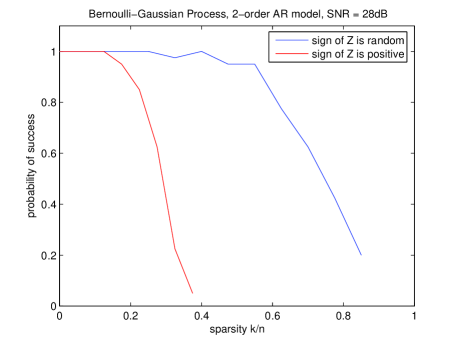
Condition (2) is new. Let us consider two scenarios. In the first scenario, each spike in can be either positive or negative with equal probability (i.e. is Bernoulli ). In this case, behaves like a sub-Gaussian sum and it is usually upper bounded by with high probability. On the other hand, let us also consider the case when all the spikes in are of the same sign, say positive. In this case each entry in and is positive and the inner product of these two aligned signals is typically much larger than the first scenario. This phenomena is also illustrated in the experiments shown in Figure 3. In the experiment, the AR model is . The blue curve corresponds to the scenario when ( is a spike) is Bernoulli . The red curve corresponds to the case when the sign of any spike is always . Each point on the curve is an average over 40 trials. We can see that in the first scenario (blue curve) we can tolerate many more spikes. To the best of our knowledge, this behavior does not exist in standard compressed sensing problem.
Theorem 2.
Denote and assume condition (1),(2) and (3) stated above are satisfied. We also assume parameter is chosen such that and , the solution to Lasso 15 is given by
| (16) | |||||
| (17) | |||||
| (18) |
and we have with probability at least .
Remark: The assumption implicitly implies an SNR bound for the smallest spike. The assumption ensures to be sufficiently large so that every non-spike element is shrunk to zero by the Lasso estimator. It is hard to analyze the case when parameter is smaller because in this case it is not clear how to construct which is critical for tractable KKT analysis. The choice of in the Theorem 2 is motivated by the proof techniques used in [17]. The proof of Theorem 2 is presented in Section 6.
4 Extensions
In this section, we provide two interesting extensions to the AR model problem. First, we generalize AR model to the autoregressive moving average (ARMA) model, i.e., the process contains both poles and zeros in the transform function. Second, we develop an algorithm for the non-causal AR process, i.e., the current state not only depends on the past inputs but also depends on the future inputs.
4.1 ARMA model
The ARMA model takes the form
| (19) |
Again we use Equation 2 to obtain the measurement where is a Toeplitz matrix as defined in Section 2. Similar to what we have done in Section 2, we write down the matrix representation of the ARMA model:
| (20) |
We denote the lower triangular matrix as
| (21) |
By multiplying to both sides of Equation 20, we get
| (22) |
Note that for ARMA model we have an additional term compared to Equation 4. Generally, matrix is unknown. We first consider a simple situation when is assumed to be known to the decoder. Based on Theorem 1 we can derive the following result. .
Theorem 3 (Known Zero Locations).
Given the same technical conditions as Theorem 1 and assume is the original sparse spike train that generates the ARMA process. Then is the unique minimizer of
| (23) |
Proof.
Note that is also a Toeplitz matrix. From the commutativity of Toeplitz matrix, we have . From Section 5, the KKT conditions claim that is the unique minimizer of Equation 23 if and only if there exists a vector such that:
-
1.
for all ,
-
2.
for all ,
-
3.
.
Applying the commutativity and define , the above three conditions are converted to
-
1.
for all ,
-
2.
for all ,
-
3.
.
Note that both the inverse and the matrix are Toeplitz. Therefore, from commutativity, the third equation is equivalent to . Finally, since is invertible, the last equation can be further simplified to . Now the KKT conditions look exactly the same as those in Section 5. Hence the corollary is proved by following the same argument as in Section 5. ∎
Now we consider the general situation when is unknown. The difficulty of decoding lies in the fact that we know neither nor the spike train . There might exist different combinations of and that matches the measurements .
Here we propose an iterative algorithm for estimating in Equation 22. Each iteration comprises of two basic steps. First, if is known (from previous iteration), we can use the following minimization algorithm to solve and (Theorem 3).
| (24) |
Here is required, even though there may not be any noise, to ensure that we do not get stuck in a local minima.
Now once is determined we switch from to , as the optimization variable. This problem reduces to a standard regression problem. First we rewrite Equation 22 as follows:
which can be simplified to where we denote
Now we formulate the following least squares optimization problem:
| (25) |
In summary our iterative algorithm consists of the following steps:
- Initialization:
-
Set , i.e., .
- Iteration :
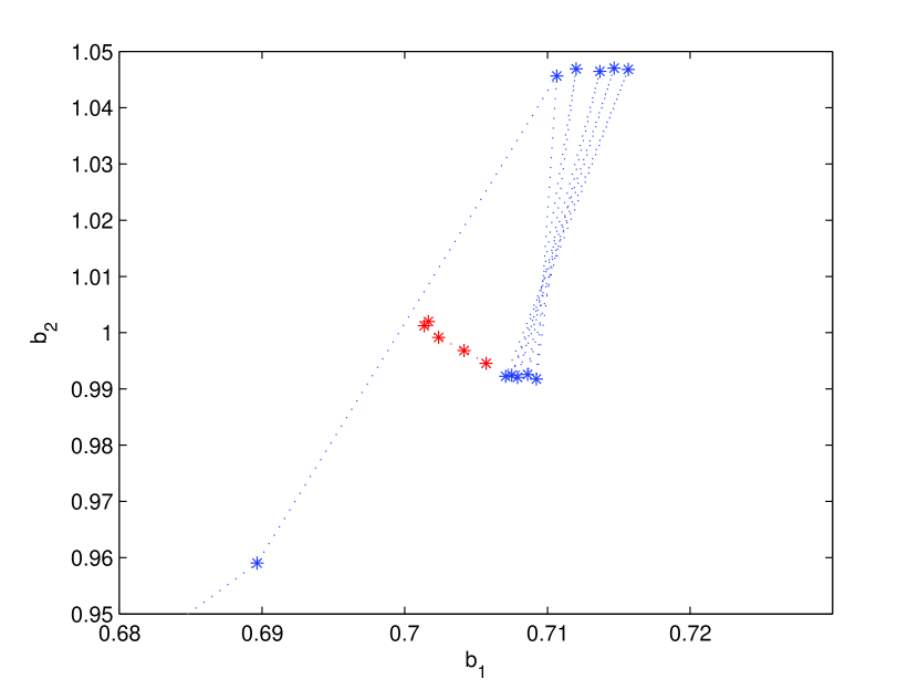
There is a subtlety in the choice of parameter in Equation 24. If is large, the iterative algorithm appears to have a faster convergence rate but at the cost of significant bias. On the other hand, if is small, the convergence rate is slow but the solution has small bias. Therefore, in practical implementation we choose to be reasonably large in the early stages of the iteration and then decrease it to at the later stages of the iteration.
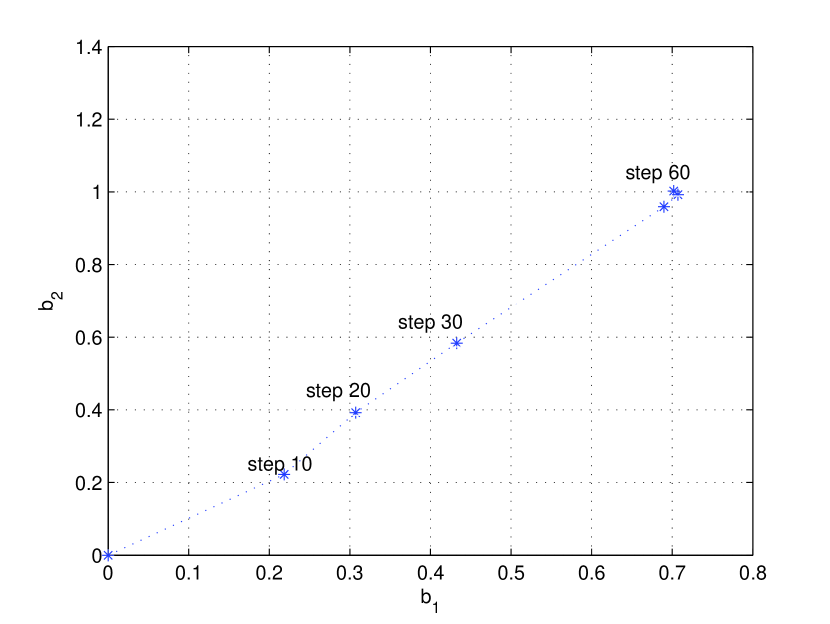
Figure 4 illustrates a concrete example of solving the ARMA model by using our iterative algorithm. We choose in the first 50 rounds of iteration and finally in the last 10 rounds of updates we set . Figure 4(b) is a zoom-in version of Figure 4(a) which shows the final stage of the algorithm. We can see the effects of choosing different value of as well.
4.2 Non-causal AR model
Many real world signals are non-causal. For example, a 2D image is usually modeled by a Markov random field, where each pixel is dependent on all its neighboring pixels. In this subsection we consider this situation by modeling the signal to be a non-causal AR process.
A non-causal AR model is defined as
| (26) |
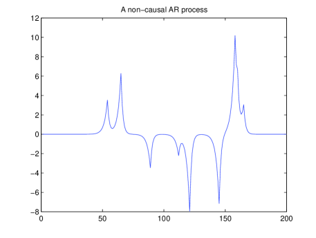
A typical non-causal AR process is shown in Figure 5. Here the impulse response of each spike is two-sided as opposed to the one-sided impulse response of causal AR process. In this subsection, we discriminate between two boundary conditions for the non-causal AR process. As we will show later, there are subtle differences in dealing with these two boundary conditions.
-
1.
Boundary is circulant, i.e., ;
-
2.
Boundary is not circulant.
4.2.1 Circulant Boundary
In this case we use the following circulant matrix in the sensing model .
| (27) |
where is i.i.d Gaussian random variable or Bernoulli random variable.
Since the boundary of is circulant (), we can write the matrix representation of Equation 26 as
| (28) |
With an abuse of notation, we use to denote the submatrix of comprising rows -th through -th of . Now we multiply to both sides of Equation 28 we get the following equation.
| (29) |
We define matrix to be
and finally Equation 29 is simplified to
| (30) |
where .
As in Section 3 we can use either -minimization or Lasso to solve this problem.
4.2.2 Non-circulant Boundary
The case of non-circulant boundary is slightly more complicated. There are two ways of handling this situation. A simple approach is to view the problem as a perturbation of the circulant boundary case, namely,
where
Now one could use Lasso to solve this noisy model:
Unfortunately, this approach will have a bias. To overcome this limitation, we consider the case where we can make an additional set of measurements corresponding to the boundary conditions, namely,
Then by the denoting
the sensing model can be simplified to the noiseless version
Again we can use either -minimization or Lasso to solve this model:
5 Proof of Theorem 1
We first write down the primal and dual formulation of algorithm 5.
| (31) |
whose dual formualtion is:
| (32) |
The proof is based on duality. is the unique minimizer of the primal problem 31 if we can find a dual vector with the following properties:
-
1.
for all ,
-
2.
for all ,
-
3.
.
where denotes the sign of ( for ) and denotes the support of vector . The above set of conditions ensure that the primal-dual pair is not only feasible but also satisfy the complementary slackness condition, thus optimal. We call the above three conditions as the Dual Optimal Condition (DOC).
The rest of this section is to construct a that satisfies the DOC. Our construction relies on the following result (see [15]).
Lemma 4 ([15]).
Let be such that , and be a real vector supported on obeying . Then there exists a vector such that . Furthermore, obeys
This lemma gives us the freedom to choose (arbitrarily) the value of in the location of while the magnitude of the rest components is still bounded.
5.1 One Pole Case
In this section we provide a proof for the simple case when is a first order AR process (i.e., ) and only contains one spike (i.e., every entry of is zero except one place). Though simple, it contains the main idea of proof techniques for the more general case. Note that in this simple case the assumptions in Theorem 1 are automatically satisfied.
For the -sparse driving process , without loss of any generality we assume and . We also denote as the root of the characteristic function of the first order AR process. Due to stability we have . Now in condition 3 of DOC, the term can be recast as
In Lemma 4, we choose as , and (). Then Lemma 4 tells us that there exists a such that and furthermore
This implies
| (33) |
where the summation . Therefore . To summarize the above discussion, we find such that:
-
1.
-
2.
for all ,
-
3.
.
Similarly, by choosing , and () in Lemma 4, there exists a such that condition 1 and 2 of DOC are also satisfied while . Hence, by convexity there exists a such that for , it satisfies and also condition 1 and 2, i.e., the whole DOC.
Finally we find a primal-dual pair that satisfy all the feasible constraints and also the complementary slackness condition, which implies is the unique minimizer of the primal problem equation 31.
5.2 General Case
In this section we prove that in the general case the three conditions in Theorem 1 ensures the existence of a that satisfies the DOC. Before giving the proof, we point out that if some conditions in Theorem 1 are violated, there might not exist such a . Let us consider the case of (first order AR process) and =2 (only two entries of are nonzero). Moreover, we choose and , that is, the two spikes are next to each other.
In this case . We pick . Clearly the assumption in Theorem 1 is broken. On the other hand, we can also check that there does not exist a that satisfies the whole DOC condition. In fact, suppose is chosen such that condition 1 and 2 are satisfied, then in checking condition 3 we find
which violates condition 3 in DOC. Hence there does not exist a that satisfies all the three conditions in DOC.
Before proving Theorem 1, we need the following lemma in constructing .
Lemma 5.
Suppose the assumptions in Theorem 1 are satisfied. Denote . Then and we also have the following inequalities:
- (1)
-
and , ,
- (2)
-
, ,
- (3)
-
and where .
Proof.
First, from the assumption of Theorem 1, . Then we need to verify the three properties.
Suppose is a new spike and be the next spike. Given , we clearly have
Hence properties (1) and (2) follow.
We denote . Therefore, for any , . Combining with the above argument, we have
Note that when as given in the theorem assumption, we have . ∎
Remark: Property (1) in Lemma 5 says
that many components of are small. Property (2) ensures that
before a new ‘spike’ begins (), the
amplitude of is already negligible (i.e.,
very close to zero) such that the new impulse response caused by
can be regarded as starting almost from zero level. Finally, property (3) says that when a new spike arrives,
the corresponding output is reasonably large compared to its neighbors.
Now we are ready to prove Theorem 1. Similar to the last section’s argument, the objective is to find a sequence of vectors such that any of satisfies the condition 1 and 2 of DOC while
and this implies there exists a convex combination which satisfies and also the condition 1 and 2 of DOC.
Based on Lemma 4, we construct via fixing the values of :
| (34) |
This choice of gives the bound . Now by applying Lemma 4, we know there exists a such that when and
where the last inequality follows from the assumption of the Theorem. Up to now we have shown that satisfies condition 1 and 2 of DOC. Next we will check the sign of .
For ,
where the magnitude of can be lower bounded,
based on property (3) of Lemma 5. And the magnitude of is upper bounded,
When as given by the assumption of the theorem, we have , which implies that the sign of is determined by the sign of .
Hence . This implies
In general, for any sign pattern , by choosing (compare equation 34) in the following way
and making similar arguments, we have
6 Proof of Theorem 2
To prove Theorem 2, we only need to check that given in the theorem satisfy the KKT conditions. We denote the function . Then the gradient of with respect to is
and the subgradient of with respect to is
where satisfies for and for . Therefore, we only need to check the following set of (in)equalities
| (35) | |||||
| (36) | |||||
| (37) |
We first check Equation 35.
Proof.
Actually,
∎
Next we check Equation 36.
Proof.
Verifying inequality 37 requires more effort. We first simplifies the formula for .
Lemma 8.
With given in Theorem 2, we have
| (39) |
where we denote as the submatrix comprises of the rows of indexed by and as the submatrix comprises of the rows of indexed by .
Proof.
Following from the proof of Lemma 7, we have ,
| (40) |
To simplify the above equation, we introduce as the matrix comprises of the rows of indexed by and the columns of indexed by . Similarly, is the matrix comprises of the rows of indexed by and the columns of indexed by ; is the matrix comprises of the rows of indexed by and the columns of indexed by . By this definition, after some column and row permutations, can be rewritten as
| (41) |
It is easy to check that and (since ). Furthermore,
Hence, Equation 40 can be simplified to
We note that can be expressed in terms of and .
Moreover can be derived via matrix inversion lemma:
Finally, we get
where (a) follows from the fact that . And similarly by repeatedly using this fact we can find the following simplification
∎
In order to justify the condition 37, we also need the following lemma.
Lemma 9.
The following three claims hold true:
- (i)
-
w.p. at least , .
- (ii)
-
w.p. at least ,
- (iii)
-
w.p. at least ,
Proof.
To prove (i), we try to bound the first component . By definition, the first column of equals . We also remember where are i.i.d. Gaussian . Hence, we have
It is easy to check that the first term of RHS is zero-mean Gaussian random variable with variance . It is well known that for standard Gaussian random variable , . So we conclude that with probability
It also can be proved that with probability
We notice that and hence claim (i) follows.
Next, we prove claim (ii). Again, can be decomposed into two terms;
The first term is bounded from the assumption and the second term is Gaussian which is bounded by (assumption (3) in Subsection 3.1) w.p. .
For (iii), we only need to show that with high probability , or where denotes the smallest singular value of .
We denote the Gaussian noise matrix
and call as the submatrix that comprises of the rows of indexed by . Then, we have
So the remaining work is to upper bound . A tight bound in this case is very difficult. However, the following bound is good enough for our proof. By denoting as the -th column of , we have
where the second last inequality follows from Cauchy-Schwartz inequality. Then by the tail probability of distribution, we have with probability ,
Then by applying assumption (1) in Subsection 3.1 we have proved the claim (iii). ∎
Finally, we can show that satisfies the condition 37.
Proof.
From the tail probability of standard Gaussian , we know that with probability at least , . Therefore the norm of all the rows of is upper bounded with probability at least . Combined with claim (iii) in Lemma 9, we know that the norm of all the rows of is upper bounded with probability at least .
Now we can verify that both and are small.
7 Numerical Experiments
We present simulations for some interesting cases. Theorem 1 asserts that as long as RIP is satisfied, stability assumptions on hold, and the spikes are well separated, our -minimization algorithm reconstructs the AR process correctly. For general IID Gaussian or Bernoulli matrix ensemble (not Toeplitz), it is well known that [9] ensures good RIP property. However, for our specific Toeplitz structured sensing matrix (Equation 2), this question (when RIP is satisfied) has not been fully answered.
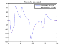
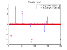
We nevertheless experiment with Toeplitz constructions. First we simulate our algorithm for a third order process. The results are depicted in Figure 6. We see that the reconstruction reproduces both the spike train as well as the filtered process accurately. For the purpose of depiction we added a small amount of noise.
(a)
(b)
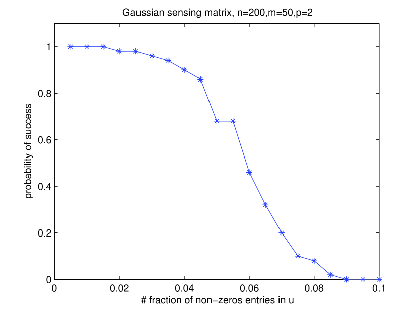
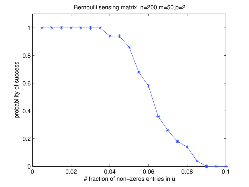
First, we fix the size of sensing matrix () and choose the entries of sensing matrix to be Gaussian. We also fix the order of the AR model () and let the sparsity vary from to . For each fixed , we run our -minimization algorithm times to obtain the average performance. The result is shown in Figure 7(a). Similarly, we can choose the sensing matrix to be Bernoulli and do the same experiment again. The result is shown in Figure 7(b). We can see that in this example Toeplitz Bernoulli matrix is more preferable than Toeplitz Gaussian matrix.
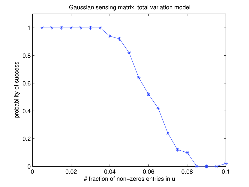
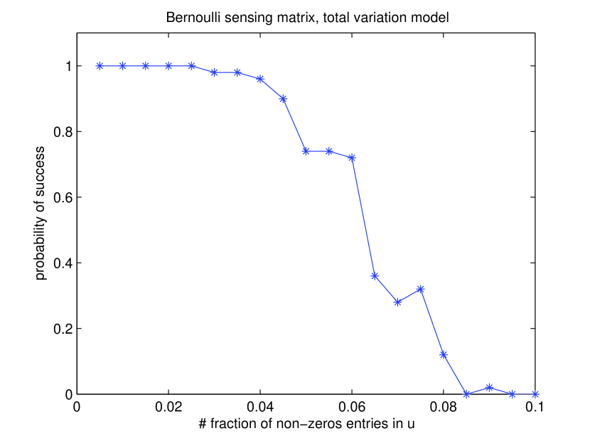
Next, we run our algorithm on a case that does not satisfy our assumptions on stability. Specifically we consider the situation when the true process is governed by the equation . This type of model is closely associated with problems that arise when one is interested in minimizing total variations. Note that in this model and it does not satisfy the assumptions of Theorem 1 where we assume . We adopt the same sensing matrix as the last experiment (Gaussian or Bernoulli) and the empirical success rate of this experiment is shown in Figure 8.
(a)
(b)
(a)
(b)
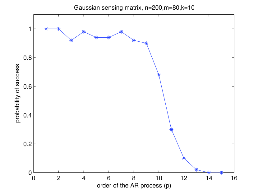
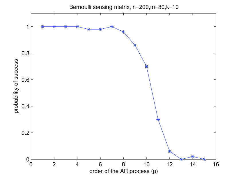
Finally we test how the order of the AR process influences the performance of the algorithm. In this experiment, we fix the size of the sensing matrix as and also fix the sparsity (i.e., the fraction of nonzero components in is ). We let (order of the AR process) vary from to . Figure 9(a) shows that empirical success rate for the Gaussian sensing matrix and Figure 9(b) shows that success rate for the Bernoulli sensing matrix. We can see that again Bernoulli Toeplitz matrix outperforms the Gaussian Toeplitz matrix.
References
- [1] E. A. Robinson, “Seismic time-invariant convolutional model,” GEOPHYSICS, vol. 50, pp. 2742–2752, December 1985.
- [2] C. Andrieu, E. Barat, and A. Doucet, “Bayesian deconvolution of noisy filtered point processes,” IEEE Transactions on Signal Processing, vol. 49, no. 1, pp. 134–146, 2001.
- [3] W. Gerstner and W. M. Kistler, Spiking Neuron Models Single Neurons, Populations, Plasticity. Cambridge University Press, August 2002.
- [4] D. L. Snyder, Random point processes. John Wiley and Sons, 1975.
- [5] J. M. Mendel, Optimal Seismic Deconvolution: An Estimation Based Approach. Academic Press, New York, 1983.
- [6] E. Cands and T. Tao, “Near optimal signal recovery from random projections: Universal encoding strategies?” preprint, 2004.
- [7] D. Donoho, “Compressed sensing,” IEEE Transactions on Information Theory, vol. 52, no. 4, pp. 1289–1306, April 2006.
- [8] ——, “For most large underdetermined systems of linear equations the minimal -norm solution is also the sparsest solution,” Communications on Pure and Applied Mathematics, vol. 59, no. 6, pp. 797–829, June 2006.
- [9] E. Cands, J. Romberg, and T. Tao, “Stable signal recovery from incomplete and inaccuarte measurements,” Communications on Pure and Applied Mathematics, vol. 59, no. 8, pp. 1207–1223, August 2006.
- [10] ——, “Robust uncertainity principles: Exact signal reconstruction from highly incomplete frequency information,” IEEE Transactions on Inforamtion Theory, vol. 52, no. 2, pp. 489–509, February 2006.
- [11] V. Saligrama, “Deterministic designs with deterministic guarantees: Toeplitz compressed sensing matrices, sequence designs and system identification,” preprint - 2008.
- [12] A. Hormati and M. Vetterli, “Annilating filter-based decoding in the compressed sensing framework,” in Wavelets XII, San Diego, California, USA, 2007.
- [13] J. A. Tropp, “Signal recovery from random measurements via orthogonal matching pursuit,” IEEE Transactions on Inforamtion Theory, vol. 53, no. 12, pp. 4655–4666, December 2007.
- [14] M. J. Wainwright, “Sharp thresholds for high-dimensional and noisy sparsity recovery using -constrained quadratic programs,” in Allerton Conference on Communication, Control and Computing, Monticello, IL, USA, 2006.
- [15] E. Cands, J. Romberg, and T. Tao, “Decoding by linear programming,” IEEE Trans. Info. Theory, vol. 51, no. 12, pp. 4203–4215, 2005.
- [16] E. Baziw and T. J. Ulrych, “Principle phase decomposition: A new concept in blind seismic deconvolution,” IEEE Transactions on Geoscience and Remote Sensing, vol. 44, no. 8, pp. 2271–2281, 2006.
- [17] E. Cands and Y. Plan, “Near-ideal model selection by minimization,” December 2007, preprint.