Supermodels for early LHC
Abstract
We investigate what new physics signatures the LHC can discover in the 2009–2010 run, beyond the expected sensitivity of the Tevatron data by 2010. We construct “supermodels”, for which the LHC sensitivity even with only 10 pb-1 is greater than that of the Tevatron with 10 fb-1. The simplest supermodels involve -channel resonances in the quark-antiquark and especially in the quark-quark channels. We concentrate on easily visible final states with small standard model backgrounds, and find that there are simple searches, besides those for states, which could discover new physics in early LHC data. Many of these are well-suited to test searches for “more conventional” models, often discussed for multi-fb-1 data sets.
I Introduction
In this paper, we explore the new physics discovery potential of the first LHC run, expected to start later this year. The latest official schedule calls for 7 TeV collisions starting in late 2009 with a ramp-up towards 10 TeV sometime during the run, which will last until late 2010 LHCrun . However, there is still some uncertainty in the ultimate center of mass energy, and the useful luminosity for physics analyses may be significantly less than the 200–300 pb-1 delivered luminosity, which is projected for this run. We therefore find it interesting to study the sensitivity of the first run as a function of LHC energy and luminosity.
In particular, it is often stated that a first LHC run with order 10 pb-1 of good data to be analyzed by ATLAS and CMS would essentially be an “engineering run” with only the capability to “rediscover” the standard model chamonix ; koeneke . One expects that order 100 pb-1 of data will be necessary for the LHC to have sensitivity to plausible new physics scenarios. Here we take a fresh look at the new physics capabilities of a 10 pb-1 low-luminosity data set, and allow ourselves to contemplate new physics which is not motivated by model building goals such as unification, weak scale dark matter, or solving the hierarchy problem.
We find that, setting such model building prejudices aside, there is a set of interesting new physics scenarios that could give rise to a clean, observable signal in early LHC data, while not being detected with 10 fb-1 of Tevatron data (roughly the projected integrated luminosity at the end of 2010). These models are consistent with previous experiments such as LEP II, precision electroweak constraints, and flavor physics. Moreover, these scenarios have similar signatures to “well-motivated” new physics models that require higher luminosity for discovery.
To set the stage, recall that the production cross sections for new hypothetical particles can be quite large. For example, QCD pair production of 500 GeV colored particles have cross sections in the pb range, such that tens of such particles could be produced in early LHC. Of course, in order for the new particles to be observable, they must have sufficiently large branching fractions to final states with distinctive signatures and controllable standard model backgrounds. Also, the new particles should not be ruled out by current or future Tevatron searches, implying that the cross section times integrated luminosity at the LHC should be larger than the corresponding quantity at the Tevatron.
Thus, the four criteria for a new physics scenario to be discovered in early LHC with low luminosity are:
-
1.
Large enough LHC cross section to produce at least 10 signal events111While fewer events might be sufficient for discovery, we shall demand 10 events to allow for uncertainties in our analysis. with 10 pb-1 of data;
-
2.
Small enough Tevatron cross section to evade the projected 2010 Tevatron sensitivity with ;
-
3.
Large enough branching fraction to an “easy” final state with essentially no backgrounds;
-
4.
Consistency with other existing bounds.
We call a new physics scenario satisfying these conditions a supermodel.
The classic example that comes to mind as a candidate supermodel is a TeV-scale boson Zprime_pdg . Assuming the mass exceeds the Tevatron reach, but is light enough and has large enough couplings so that it can be produced copiously at the LHC, then it can be discovered through its decay to electron and muon pairs. Such leptonic finals states are “easy” to reconstruct with a peak in the invariant mass distribution, which reduces the already low standard model backgrounds.
As we will see, however, a typical leptonically decaying is actually not a supermodel. First, since the is produced via the quark-antiquark initial state, the Tevatron is quite competitive with the LHC. Second, the leptonic branching fraction is severely bounded by LEP II data, which restricts the couplings of the to leptons. It is therefore nontrivial to find supermodels that are as discoverable as a standard but consistent with known bounds on new physics.
The remainder of the paper is organized as follows. In Sec. II, we identify new particle production channels with sufficiently large LHC cross sections and for which the LHC has an advantage over the Tevatron. Assuming perturbative couplings, we find that -channel production of quark-quark () or quark-antiquark () resonances are the best starting points for early LHC supermodels. In Sec. III, we construct explicit models where these resonances can decay to interesting and easily reconstructable final states. While a standard does not work, generalized scenarios can be supermodels, as are scenarios involving diquarks. We conclude in Sec. IV.
II Production Modes
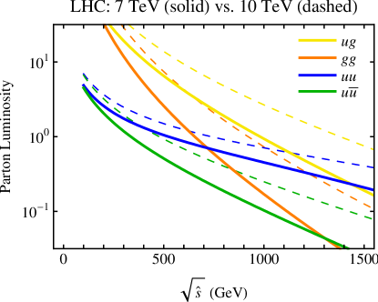
In this section, we discuss which production modes have the potential to be supermodels, deferring detailed model building to Sec. III. Since the expected integrated luminosity at the Tevatron () is orders of magnitude larger than our benchmark luminosity for early LHC analysis, and since parton luminosities are not so different from parton luminosities, one must consider sufficiently heavy new particles to evade the Tevatron reach. We will find that the most promising perturbative scenarios accessible with 10 pb-1 of LHC data are and resonances.
To begin, we plot in Fig. 1 the LHC parton luminosities, defined as
| (1) |
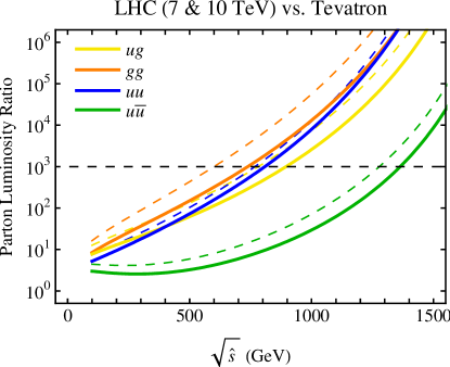
and in Fig. 2 the ratios of each parton luminosity at the LHC and the Tevatron. In Eq. (1), is the center of mass energy of the collider, is the invariant mass of the two interacting partons, and are the parton distribution functions evaluated at a momentum fraction and scale . We use the CTEQ-5L parton distribution functions Lai:1999wy . (For similar plots using CTEQ-6L1 Pumplin:2002vw , see Ref. Quigg:2009gg .)
It is often stated that the LHC is essentially a gluon collider, so one might think that processes initiated by gluons would be the best starting points for constructing supermodels. However, Fig. 1 shows that the parton luminosity only dominates for small invariant mass, where the initial LHC data set cannot compete with the Tevatron. As seen in Fig. 2, only at large invariant masses do the LHC parton luminosities become sufficiently enhanced compared to the Tevatron. (The enhancement of the channel is the smallest, so it is harder for the LHC to compete in cases where the initial state contributes.) To build supermodels, we must explore the possible LHC cross sections in the region with large enough enhancements compared to the Tevatron. We will emphasize this point in the next subsection by showing why QCD pair production is not a supermodel, and then go on to consider supermodels constructed from -channel resonances.
II.1 QCD pair production?
A simple process initiated by gluons is QCD pair production of new colored particles. For not too heavy states, it can have a cross section above a pb, yielding events with 10 pb-1 of LHC data. However, it is easy to show that such processes are generically not supermodels. For concreteness, we study the production of a color-triplet quark . We assume that it always decays to a highly visible final state, and that reconstruction efficiencies are perfect. One can then use the standard QCD diagrams to calculate the largest value of for which the Tevatron would observe 10 pair production events with 10 fb-1 of data. In this idealized example, the hypothetical Tevatron bound is . The same exercise can be repeated for the LHC as a function of the center of mass energy and integrated luminosity, and the result is shown in Fig. 3.
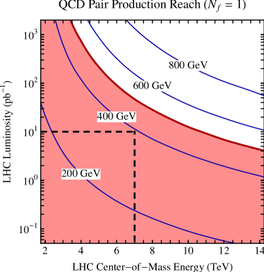
To reach the Tevatron sensitivity for QCD pair production at a 7 TeV LHC, the required luminosity is about 50 pb-1. While this is likely within the reach of an early LHC run, the LHC will not easily surpass Tevatron bounds in this channel, and it is unlikely that a 5 LHC discovery is possible without the Tevatron already having seen some events. (The same holds for colored scalar pair production Manohar:2006ga ; Dobrescu:2007yp ; Burgess:2009wm .) This conclusion is only bolstered when realistic branching fractions to visible final states and signal efficiencies are taken into account.
The primary reason why QCD pair production is not a supermodel is that the same final state can also be produced from the initial state, where the LHC has less of an advantage over the Tevatron. The situation can be improved if there is a large multiplicity of near-degenerate new colored states or if the new states are color octets (like gluinos in supersymmetry). Then the total cross sections are larger by a multiplicity factor and the LHC reach can surpass that of the Tevatron (where the cross section is more strongly suppressed at higher masses). As an example, leptoquark pair production Leptoquark_pdg yields the easily reconstructable final state of two leptons and two jets, so this could be a supermodel with a sufficiently large multiplicity of such leptoquarks.
In any case, because QCD pair production is quite well-studied in specific new physics scenarios and because the early LHC advantage over the Tevatron can only be marginal, we will not consider it to be a supermodel in this paper. In Sec. III.5, though, we show that pair production through an intermediate resonance can give rise to supermodels.
II.2 Resonance production
While pair production of new colored particles is not a supermodel, production of an -channel resonance has the potential to be a supermodel, as long as the resonance has renormalizable couplings to the partonic initial states. Recall that parametrically the production cross section for a single resonance is enhanced over pair production by a phase space factor of . Moreover, unlike QCD pair production where gauge invariance relates the and scattering amplitudes, single resonance production can be dominated by one partonic initial state.
In the narrow width approximation, we can parametrize generic single resonance production by
| (2) |
where denote the two partons which participate in the hard scattering, is the mass of the resonance, and encodes all information about the production of resonance from the two partons, including couplings, polarization, and color factors. Using the parton luminosities defined in Eq. (1), the hadronic cross section is
| (3) |
For the resonances considered in this paper, one production channel dominates, allowing us to drop the label from .
For reasonably narrow resonances with dimension four couplings, can be order , which is the case for the and initial states. However, for the or initial states gauge invariance forbids renormalizable couplings to a single resonance. For example, for the initial state, the lowest dimension operator allowed is a dimension five coupling to a scalar or pseudoscalar:
| (4) |
The coefficient of the operator has been estimated assuming perturbative physics at TeV, with the factor coming from a loop. This gives a rather suppressed effective coupling , where we have assumed is around a TeV. If there is strong dynamics involving at the TeV scale, then the coefficient in Eq. (4) can be enhanced up to its naive dimensional analysis value . However, such strong dynamics near the TeV scale is constrained by precision measurements, and we will adopt the perturbative estimate for both and resonances.
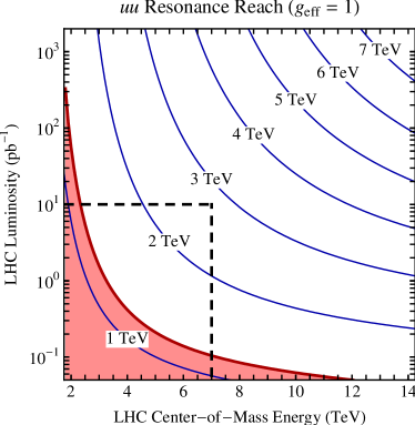
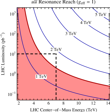
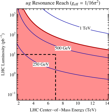
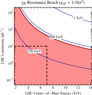
In Fig. 4, we show our estimate of the generic early LHC reach in , as a function of the energy and luminosity, for the four resonance channels using
| (5) |
As in Fig. 3, we assume 100% branching fraction of to highly visible final states and assume perfect detector efficiency, though we will relax these assumptions below. Note that for a charged resonance (that is produced from and initial states), the search strategy for the charge conjugate resonance arising from and initial states is equivalent, and any analysis will include both. The plots in Fig. 4 use the quark parton distribution function for simplicity (rather than that of the or both) and include the and initial states instead of and only.
We see that while gluons are by far the most abundant partons at small , scattering initiated by gluons does not lead to very large resonance cross sections at the LHC, if perturbative couplings are assumed. In the and especially in the channels, shown in the two upper plots of Fig. 4, the first LHC run even with modest energy and luminosity will supersede the Tevatron. Thus, and resonances are the most suitable starting points for constructing supermodels, examples of which will appear in Sec. III.
II.3 Production of and resonances
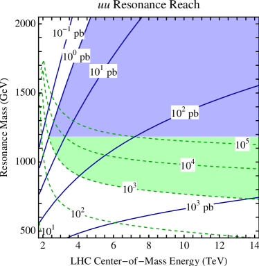
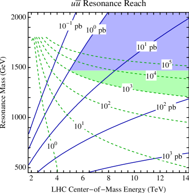
The plots in Fig. 4 give a rough idea of the LHC discovery potential for -channel resonances. They are valid for a particular value of the effective coupling, , and assume that the resonance is observed with 100% efficiency. For the two most promising scenarios of and resonances, we are interested in the dependence of the reach on and on branching fractions/efficiencies. Here, we introduce a new kind of plot which is convenient for reading off cross sections at the LHC and comparing them to the Tevatron for variable couplings and detection efficiencies. In Fig. 5, we plot in the LHC energy vs. resonance mass plane the contours of constant production cross section and contours of constant ratio of LHC vs. Tevatron cross section.
The solid curves (with positive slopes) in Fig. 5 show contours of constant LHC cross sections for . From these, one can read off how many events are produced for a given LHC luminosity as a function of the resonance mass and the LHC energy. For example, assuming 100% visible decay rate and detection efficiency, the region to the right of the curve labeled “ pb” will yield at least 10 events with of LHC data. For a concrete model, with a different value of , branching ratio to easily reconstructable final state(s), and detector/reconstruction efficiency , the LHC with a given energy and luminosity can see or more events to the right of the solid curve labeled
| (6) |
For example, if and , then 10 or more events can be observed in the region to the right of the curve labeled “ pb” (“ pb”) with 10 pb-1 (100 pb-1) of LHC data.
The dashed curves (with negative slopes) in Fig. 5 show contours of constant ratio of LHC vs. Tevatron cross sections. From these, one can read off the relative advantage of the LHC compared to the Tevatron for a given model. For many resonances, the same initial state dominates the production of a resonance at the Tevatron and the LHC, so that the factors of cancel in the ratio of the two cross section. If, in addition, the same final states are searched for at the Tevatron and at the LHC and the detection efficiencies are similar, then these cancel in the ratio as well. Therefore, the LHC has better sensitivity than the Tevatron in the region above the dashed curve labelled by
| (7) |
For example, the LHC with (100 pb-1) will produce more events than the Tevatron with in the region above the dashed curve labeled “” (“”). Any significant differences in detection efficiencies between the two colliders can easily be included by multiplying Eq. (7) by .
Thus, it is a “wedge” bounded by a solid and a dashed curve which defines the region in which the LHC has better sensitivity than the Tevatron and yields at least a certain number of events. For example, the wedge to the right of the intersection of the “ pb” and the “” curves gives the region for which at least 10 events are produced with of LHC data and the number of events at the LHC is greater than that at the Tevatron. These regions are shaded in Fig. 5. (To include model specific effects, replace the “ pb” solid curve by the one.)
At the intersection of a solid and a dashed curve, the ratio of their labels gives the Tevatron cross section, and can be used to estimate the Tevatron discovery reach. The intersection of any “ pb” solid curve with a “” dashed curve corresponds to the same fixed Tevatron cross section of pb for arbitrary . Since the Tevatron cross section does not depend on the LHC energy, these intersections lie on a horizontal line. The corresponding value of the resonance mass is the one for which the Tevatron with 10 fb-1 data produces events. For example, for masses below the straight line across the intersection of the “ pb” and the “” curves (i.e. ), the Tevatron will also produce at least 10 events with 10 fb-1 data. While everywhere in the full wedges shaded in Fig. 5 the LHC sensitivity is better than that of the Tevatron, below this straight line the Tevatron sensitivity is good enough that it can make a discovery prior to the LHC.222For a sequential decaying to leptons, taking , this predicts a 10 fb-1 Tevatron bound near 1.2 TeV; crude, but reasonable Aaltonen:2008ah . Therefore, it is only the part of the “wedge” above this straight line, shaded blue, which is the true LHC discovery region.
Using these plots, one can also estimate the minimum value of and for a scenario to be a supermodel. Take a resonance as an example. A 7 TeV and pb-1 early LHC run supersedes the Tevatron sensitivity for a TeV (the value of the “” dashed curve at 7 TeV). We can then read off that is required to observe at least 10 events. For larger initial LHC luminosity, this minimum of course gets smaller.


(A) (B) (C)
III Example Supermodels
Considering production cross sections alone, and resonances emerged as the two best starting points for constructing early LHC supermodels. In this section, we consider concrete supermodel examples to see what kind of final states can be obtained from the decay of these resonances. Since we are interested in final states that involve the cleanest signatures and least background contamination, we concentrate on decay chains yielding (at least) two charged leptons (or two other stable charged particles) in the final state.
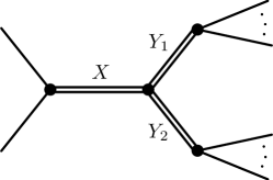
Because there is a plethora of possible decay patterns for a or resonance, we find it convenient to classify the decay modes of new resonances in terms of three basic decay topologies, which often appear in perturbative new physics scenarios. These are depicted in Fig. 6. Double lines denote new resonances and solid lines are detectable final states, either standard model particles or new (quasi-)stable states.
-
•
Topology A: The resonance decays directly to two detectable final state particles. Note that a three-body decay for the resonance will generically not compete with the decay back to QCD partons, since the branching fraction to a three-body final state is suppressed by a phase space factor compared to the two-body decay channel back to the initial state.
-
•
Topology B: The resonance decays to one detectable final state and one new secondary resonance . Subsequently can decay to two or more standard model particles. Note that always has a decay mode back through the production diagram with a virtual .
-
•
Topology C: The resonance decays to two new secondary resonances and , possibly of different masses. These secondary resonances can each decay to two or more detectable states. This topology can be used for example to “resurrect” pair production of colored particles as a supermodel.
The classic case of topology A is a leptonically decaying , and this is often described as the simplest new physics channel to discover at a hadron collider. However, we will argue below that a standard is not a supermodel if one takes into account the indirect constraints coming from LEP II. After dismissing the standard case, we will give a (non-exhaustive) list of supermodels exhibiting the three above topologies.
While some of the example supermodels are simple variants on well-motivated models, the case of a resonance (or diquark) is less well-known (though we will show that such a particle can arise in the minimal supersymmmetric standard model; see also Ref. Angelopoulos:1986uq ). Despite the unfamiliar quantum numbers of the diquark, the final states achievable in diquark decays can be shared by more familiar resonances, albeit with smaller non-supermodel cross sections. In this way, searches for supermodels in early LHC data can anticipate searches that require higher luminosity.
For reference, the standard model quantum numbers are:
|
(8) |
III.1 The case against a standard
For a resonances to be supermodel, it must have a large branching fraction to visible final states. In particular, since a resonance can have zero electric charge, it is natural for such a resonance to decay via topology A to pairs of oppositely charged leptons, in particular and . However, the same resonance also induces a low energy effective four-lepton vertex, and such operators are severely constrained by LEP II. As recently emphasized in Ref. Salvioni:2009mt , once the LEP II bound is imposed, the branching fraction of the resonance to has to be too small to realize a supermodel.
As a concrete example, consider a new gauge boson :
|
(9) |
with couplings to standard model fermions of the form333Here and below, we use 2-component fermion notation.
| (10) |
where are the corresponding coupling constants. For simplicity, imagine a common coupling to quarks and to leptons.444While such a choice of charges is typically anomalous (unless ), such anomalies can always be canceled with new fermions (spectators) whose masses result from the same symmetry breaking which gives the its mass.
In the narrow width approximation, the production cross section for this resonance is
| (11) |
and the branching ratio of this to charged leptons is555We are assuming Dirac neutrino masses for definiteness, and we do not consider final state ’s to be easily reconstructable, hence the overall factor of .
| (12) |
The coupling to to leptons is strongly constrained by LEP II limits on four-fermion operators Alcaraz:2006mx ,
| (13) |
Putting this together, we find
| (14) |
Using Fig. 5 and Eq. (6), one finds that there is no value of for which 10 events could be seen with of data, even with a center of mass energy of 14 TeV.
There are ways to evade this conclusion. Since the LEP II bound only applies for the electron coupling, one could imagine coupling the only to muons. However, such flavor non-universal couplings typically require significant fine-tuning to avoid constraints from flavor changing neutral currents. Alternatively, one might consider the production of a -like resonance, i.e., a resonance with electric charge 1, which decays to a charged lepton and a neutrino. However, typically such models have an accompanying -like state, which faces the strong LEP II bounds.
III.2 Decays to quasi-stable particles
While the decay of a to standard model charged leptons does not give a viable supermodel example of topology A, one could imagine a resonance that instead decayed with a large branching fraction to new quasi-stable charged particles. Since ATLAS and CMS trigger on penetrating charged particles as if they were muons Fairbairn:2006gg , such scenarios are as visible in the early LHC data as a decaying to muons.
One simple choice is to take the above boson with , and introduce vector-like “leptons”, and , with coupling to the and non-zero electric charge.
|
(15) |
The and fields can have an approximate symmetry to make them long-lived, but they must eventually decay to avoid cosmological bounds on absolutely stable charged relics. For this reason, the hypercharge for and has been chosen such that the quasi-stable lepton can decay via mixing with the standard model .
The branching fraction of the to the stable charged states is
| (16) |
For large enough values of , the branching fraction can be order 1. Because the stable “leptons” are being produced from a resonance, they will typically have a velocity of
| (17) |
so depending on the relevant mass ratio , a standard “slow muon” cut of CMS_stable_charged will not be particularly effective at capturing the signal. In such cases, these stable charged particles should be treated like ordinary muons (without imposing any kind of quality cut tailored to muons) to reconstruct a resonance.
Alternatively, one could consider a that decayed to quasi-stable colored particles that then form -hadron-like bound states with QCD partons. Such -hadron final states could potentially be visible in early LHC data, though charge flipping interactions Fairbairn:2006gg complicate both triggering and momentum reconstruction.
III.3 Fun with diquarks
From Fig. 5, one sees that resonances can yield an impressive early LHC reach. Such resonances are known as diquarks, and they have spin zero or one, carry baryon number 2/3, and electric charge 4/3, 1/3 or 2/3. They may transform as a or of color. Their couplings are necessarily non-trivial in flavor space because the initial quarks carry flavor. Flavor changing neutral currents impose constraints on couplings of new states with masses of order TeV and large couplings to first generation quarks. To be safe, we consider diquarks with the same flavor quantum numbers as the quarks which produce them, allowing the couplings of the diquark to quarks to be flavor invariant. (Other models Chacko:1998td consider a single diquark which couples to the quarks with a Yukawa matrix, and generically lead to dangerous flavor violation.)
To be concrete, we consider a spin-zero and color-six diquark, with couplings to the singlet up-type quarks only and symmetric in flavor indices.666We discuss the phenomenology of a color-triplet diquark which occurs naturally in the context of R-parity violating SUSY in the next subsection.
|
(18) |
The production operator can be written as
| (19) |
where are the up-type singlet quarks and is the diquark. The normalization of the coupling constant depends on the normalization of the color matrices with which we expand . We use orthonormal matrices such that . Then the partonic cross section is777Recently radiative corrections were calculated, giving a -factor of 1.3 Mohapatra:2007af .
| (20) |
If Eq. (19) were the only available coupling for the diquark, then any produced diquark would simply decay back to the initial state with a partial width given by . To be a supermodel, the diquark has to have a large branching fraction to a visible final state. By color conservation, diquark decays must yield at least two jets in the final state, so the most -like decay possible for a diquark (in the sense that it yields two oppositely charged leptons in the final state) is
| (21) |
Such a final state can appear via topology B or C, though we will consider the case of topology B since it requires fewer new degrees of freedom.
For example, we can introduce a vector-like fermion and , with the quantum numbers:
|
(22) |
Given its quantum numbers, / would be called a “leptodiquark”. The diquark can then decay via the operator
| (23) |
with a decay width of . Thus, as long as , the diquark preferentially decays to the leptodiquark and a lepton. The will finally decay via the operators in Eqs. (19) and (23) as
| (24) |
through an off-shell diquark, leading to the full decay chain:
| (25) |
The final state therefore has two jets plus an opposite sign lepton pair, arranged in topology B.
While this diquark-leptodiquark system may strike the reader as baroque, the identical decay topology appears in the case of a gauge boson Aad:2009wy ; Ball:2007zza , where the diquark plays the role of the and the leptodiquark plays the role of a right-handed neutrino. However, discovering a left-right symmetric model through this channel typically requires Aad:2009wy ; Ball:2007zza of LHC data, whereas the diquark-leptodiquark example motivates a search for the final state in early LHC data.
III.4 Squarks as diquarks
A curious example of a supermodel with diquarks is the MSSM with -parity violation. The superpotential term , where and are chiral superfields, allows for resonant production of a single squark in the scattering of two quarks Dimopoulos:1988fr . The coupling constants are constrained by flavor physics, oscillations, and double-nucleon decays. However for squark masses of order 1 TeV or larger, couplings of order one for and are allowed Goity:1994dq ; Allanach:1999ic .
Such order one couplings give a very large cross section for single squark production in scattering. Contours of these cross sections are similar to what is shown in the left panel of Fig. 5 for scattering. The produced squarks ( or ) have order one branching fractions to decay back into dijets by the inverse of the production process. More interestingly, they also have large branching fractions to decay via one of the typical SUSY cascade decays ending in the lightest superpartner (LSP). The decay chains depend on the details of the superpartner spectrum.
For example, if the order of superpartner masses from heaviest to lightest is squarks gluinos gauginos sleptons bino, then the squark would usually decay into its corresponding quark and the gluino. This decay can beat the decay back to jets because of the large QCD coupling and the color factor associated with the gluino. A typical whole decay chain yielding final state leptons would be an extended version of topology B:
| (26) |
where the LSP decay into 3 jets in the last step proceeds via an off-shell squark using the -parity violating vertex. This decay chain of course assumes that the gluino itself does not decay to 3 jets via the -parity violating operator.
Even with a SUSY cascade decay, it is not guaranteed to get visible leptons in the final state. For example, a superpartner spectrum of the form gluinos squarks gauginos sleptons bino, would typically produce a much shorter SUSY decay chain, ending with a four jet final state and no leptons. This is because the produced squark is an singlet which decays directly into a quark and the bino (the LSP), with the bino eventually decaying to three quarks. One can get copious lepton production with a slepton LSP, and the spectrum gluinos squarks gauginos bino sleptons would give
| (27) |
Finally, a spectrum where left- and right-handed sleptons alternate with neutralinos can even give rise to four leptons in addition to several jets.
III.5 Resurrecting pair production
In Sec. II.1, we argued that QCD pair production of new colored resonances was not a supermodel. However, topology C allows for pair production of new resonances via a supermodel resonance.
For example, using either a or a resonance, one can produce vector-like up-type quarks and with quantum numbers:
|
(28) |
They can be produced via the through
| (29) |
or via the diquark through
| (30) |
If these new colored particles were exactly stable, they would form -hadron-like bound states as mentioned above, leading to topology A. However, the heavy quarks may decay via small CKM-like mixings with the standard model quarks, leading to
| (31) |
Such decays are not ideal for making a supermodel, since the () boson only has 22% (7%) branching fraction to electrons and muons. However, if the quarks only couple to other standard model fermions through higher-dimension operators like
| (32) |
then each decay can lead to leptons via
| (33) |
Operators like Eq. (32) can always be generated through sufficiently creative model building, and the scale can be made sufficiently large to evade flavor constraints while still being small enough to give prompt decay.
Another option to force leptons to appear in the final state is to have a resonance decay to pairs of colored particles that also carry lepton number, such as leptoquarks or even the leptodiquarks of Eq. (22).888To produce such states from the diquark resonance, one needs two different fields of opposite lepton number but same baryon number, i.e. a leptoquark and an antilepto-quark. Alternatively, through a resonance, one can pair produce color singlet objects with lepton number, such as “sleptons” Baumgart:2006pa , as long as the resonance does not couple to standard model leptons directly.
Finally, a neutral resonance can dominantly decay to two secondary resonances that carry no standard model charges. These secondary resonances have a near infinity of possible decay modes, opening up a huge range of final state possibilities. Such scenarios will be supermodels as long as the secondary resonances have an branching fraction to highly visible final states.
IV Conclusions
In this paper, we investigated some new physics scenarios which could be probed by a low energy and low luminosity initial LHC data set, and which will not have been ruled out by the Tevatron and other measurements. We call such scenarios supermodels; they are not necessarily motivated by usual model building goals such as solving the hierarchy problem, but are constructed to demonstrate that high production cross sections and clean experimental signatures are possible for early LHC.
Assuming perturbative couplings, we found that -channel production of or resonances are the most promising supermodel scenarios. To supersede the Tevatron sensitivities in searches for pair-produced particles or single resonances produced from an initial state involving gluon(s), the LHC typically needs higher integrated luminosity than considered in this paper. Not unexpectedly, given a collider, we found that resonances that couple to initial states have by far the largest LHC cross sections, and in this channel there is a large space of supermodels (see Fig. 5).
We explored various decay topologies of the produced resonances that lead to easily identifiable final states containing a pair of charged leptons or other (quasi-)stable charged particles. While the possibilities for such decays are only limited by theorists imagination and model building ingenuity, we presented some simple examples focusing on decay topologies that also arise in more standard extensions of the standard model. While the supermodels exhibited here might not be as attractive as the name suggests, many of the same final state signatures are useful search channels for “well motivated” models as well. Therefore, searching for supermodels with the early LHC data may benefit finding prettier models when larger data samples become available.
Finally, the space of interesting early LHC searches would be extended if (i) nonperturbative couplings are considered; (ii) pair production is enhanced by high particle multiplicities; (iii) one compares to the currently published Tevatron bounds (some of which utilize less than 100 pb-1 of data) instead of the 2010 Tevatron sensitivity with 10 fb-1 of data; (iv) the early LHC data used for analysis approaches or goes beyond 100 pb-1.
Acknowledgements.
We thank Mina Arvanitaki, Beate Heinemann, and Matthew Schwartz for helpful conversations. This work was supported in part by the Director, Office of Science, Office of High Energy Physics of the U.S. Department of Energy under contract DE-AC02-05CH11231. M.S. is supported by DE-FG02-01ER-40676. J.T. acknowledges support from the Miller Institute for Basic Research in Science. D.W. was supported by a University of California Presidential Fellowship. M.S. and J.T. thank the Aspen Center for Physics for their hospitality while this work was in preparation.References
- (1) CERN press release, http://press.web.cern.ch/press/PressReleases/Releases2009/PR13.09E.html; H. Burkhardt, Status of the LHC Machine, Lepton-Photon 2009, Hamburg, Germany, 16–22 August 2009, https://indico.desy.de/getFile.py/access?contribId=0&sessionId=3&resId=0&materialId=slides&confId=1761.
- (2) Proceedings of the 2009 Chamonix workshop on LHC performance, CERN-ATS-2009-001, https://espace.cern.ch/acc-tec-sector/Chamonix/Chamx2009/html/session.htm.
- (3) K. Koeneke, Early Physics Measurement at the LHC with ATLAS, http://cdsweb.cern.ch/record/1205269
- (4) See the review “-boson searches” in C. Amsler et al. [Particle Data Group], Phys. Lett. B 667, 1 (2008).
- (5) H. L. Lai et al. [CTEQ Collaboration], Eur. Phys. J. C 12, 375 (2000) [arXiv:hep-ph/9903282].
- (6) J. Pumplin, D. R. Stump, J. Huston, H. L. Lai, P. M. Nadolsky and W. K. Tung, JHEP 0207, 012 (2002) [arXiv:hep-ph/0201195].
- (7) C. Quigg, arXiv:0908.3660 [hep-ph].
- (8) A. V. Manohar and M. B. Wise, Phys. Rev. D 74, 035009 (2006) [arXiv:hep-ph/0606172].
- (9) B. A. Dobrescu, K. Kong and R. Mahbubani, Phys. Lett. B 670, 119 (2008) [arXiv:0709.2378 [hep-ph]].
- (10) C. P. Burgess, M. Trott and S. Zuberi, arXiv:0907.2696 [hep-ph].
- (11) See the review “Leptoquarks” in C. Amsler et al. [Particle Data Group], Phys. Lett. B 667, 1 (2008).
- (12) T. Aaltonen et al. [CDF Collaboration], Phys. Rev. Lett. 102, 091805 (2009) [arXiv:0811.0053 [hep-ex]].
- (13) V. D. Angelopoulos, J. R. Ellis, H. Kowalski, D. V. Nanopoulos, N. D. Tracas and F. Zwirner, Nucl. Phys. B 292, 59 (1987).
- (14) E. Salvioni, G. Villadoro and F. Zwirner, arXiv:0909.1320 [hep-ph].
- (15) J. Alcaraz et al. [The LEP Collaborations ALEPH, DELPHI, L3, OPAL, and the LEP Electroweak Working Group], arXiv:hep-ex/0612034.
- (16) M. Fairbairn, A. C. Kraan, D. A. Milstead, T. Sjostrand, P. Skands and T. Sloan, Phys. Rept. 438, 1 (2007) [arXiv:hep-ph/0611040].
- (17) The CMS Collaboration, CMS PAS EXO-08-003 (2008) http://cms-physics.web.cern.ch/cms-physics/public/EXO-08-003-pas.pdf.
- (18) Z. Chacko and R. N. Mohapatra, Phys. Rev. D 59, 055004 (1999) [arXiv:hep-ph/9802388]; K. S. Babu, R. N. Mohapatra and S. Nasri, Phys. Rev. Lett. 97, 131301 (2006) [arXiv:hep-ph/0606144]; K. S. Babu, P. S. Bhupal Dev and R. N. Mohapatra, Phys. Rev. D 79, 015017 (2009) [arXiv:0811.3411 [hep-ph]]; C. R. Chen, W. Klemm, V. Rentala and K. Wang, Phys. Rev. D 79, 054002 (2009) [arXiv:0811.2105 [hep-ph]].
- (19) R. N. Mohapatra, N. Okada and H. B. Yu, Phys. Rev. D 77, 011701 (2008) [arXiv:0709.1486 [hep-ph]]; T. Han, I. Lewis and T. McElmurry, arXiv:0909.2666 [hep-ph].
- (20) G. Aad et al. [The ATLAS Collaboration], arXiv:0901.0512 [hep-ex].
- (21) G. L. Bayatian et al. [CMS Collaboration], J. Phys. G 34 (2007) 995.
- (22) S. Dimopoulos, R. Esmailzadeh, L. J. Hall and G. D. Starkman, Phys. Rev. D 41, 2099 (1990).
- (23) J. L. Goity and M. Sher, Phys. Lett. B 346, 69 (1995) [Erratum-ibid. B 385, 500 (1996)] [arXiv:hep-ph/9412208].
- (24) B. C. Allanach, A. Dedes and H. K. Dreiner, Phys. Rev. D 60, 075014 (1999) [arXiv:hep-ph/9906209].
- (25) M. Baumgart, T. Hartman, C. Kilic and L. T. Wang, JHEP 0711, 084 (2007) [arXiv:hep-ph/0608172].