A Measurement of Small Scale Structure in the $2.2\leq z\leq 4.2$ Lyman-alpha Forest

Abstract

The amplitude of fluctuations in the Lyman-alpha (Ly-$\alpha$) forest on small spatial scales is sensitive to the temperature of the intergalactic medium (IGM) and its spatial fluctuations. The temperature of the IGM and its spatial variations contain important information about hydrogen and helium reionization. We present a new measurement of the small-scale structure in the Ly-$\alpha$ forest from 40 high resolution, high signal-to-noise, VLT spectra for absorbing gas at redshifts between $2.2\leq z\leq 4.2$. We convolve each Ly-$\alpha$ forest spectrum with a suitably chosen Morlet wavelet filter, which allows us to extract the amount of small-scale structure in the forest as a function of position across each spectrum. We monitor contamination from metal line absorbers. We present a first comparison of these measurements with high resolution hydrodynamic simulations of the Ly-$\alpha$ forest which track more than 2 billion particles. This comparison suggests that the IGM temperature close to the cosmic mean density ($T_{0}$) peaks at a redshift near $z=3.4$, at which point it is greater than $20,000$ K at $\gtrsim 2-\sigma$ confidence. The temperature at lower redshift is consistent with the fall-off expected from adiabatic cooling ($T_{0}\propto(1+z)^{2}$), after the peak temperature is reached near $z=3.4$. In our highest redshift bin, centered around $z=4.2$, the results favor a temperature of $T_{0}=15-20,000$ K. However, owing mostly to uncertainties in the mean transmitted flux at this redshift, a cooler IGM model with $T_{0}=10,000$ K is only disfavored at the 2-$\sigma$ level here, although such cool IGM models are strongly discrepant with the $z\sim 3-3.4$ measurement. We do not detect large spatial fluctuations in the IGM temperature at any redshift covered by our data set. The simplest interpretation of our measurements is that HeII reionization completes sometime near $z\sim 3.4$, although statistical uncertainties are still large. Our method can be fruitfully combined with future HeII Ly-$\alpha$ forest measurements.

1. Introduction

A key characteristic in our description of the baryonic matter in the Universe is the thermal state of the gas in the intergalactic medium (IGM). As such, detailed constraints on the temperature of the gas in the IGM, its spatial variation, density dependence, and redshift evolution, are of fundamental importance to observational cosmology. During the Epoch of Reionization (EoR), essentially the entire volume of the IGM becomes filled with hot ionized gas. The thermal state of the IGM subsequently retains some memory of when and how the intergalactic gas was ionized (Miralda-Escude & Rees 1994, Hui & Gnedin 1997), owing to the long cooling times for this low density gas. Measurements of the thermal history of the IGM hence translate into valuable constraints on the reionization history of the Universe (e.g. Theuns et al. 2002a, Hui & Haiman 2003).

Current observations suggest that there may in fact be two separate EoRs: an early Epoch of Hydrogen Reionization during which hydrogen is ionized, and helium is singly-ionized, by star-forming galaxies, followed by a later Epoch of Helium Reionization during which helium is doubly ionized by bright quasars (e.g. Madau et al. 1999). Recent measurements of the quasar luminosity function (Hopkins et al. 2007), combined with estimates of the quasar spectral shape and the clumpiness of the IGM, suggest that HeII reionization may complete somewhere near $z\sim 3$ (Furlanetto & Oh 2008, Faucher-Giguère et al. 2008a, McQuinn et al. 2008). Indeed, there are some observational indications that helium is doubly-ionized close to $z\sim 3$ (see e.g., Schaye et al. 2000, Furlanetto & Oh 2008, Faucher-Giguère et al. 2008a, McQuinn et al. 2008 for a discussion), although the evidence is generally weak and controversial.

Further detailed studies of the HI Ly-$\alpha$ forest near $z\sim 3$ offer promise to pin-point when HeII reionization occurs and can potentially constrain properties of HeII reionization, such as the filling factor and size distribution of HeIII regions at different stages of reionization. Photoheating during HeII reionization impacts the thermal state of the IGM (e.g., Miralda-Escude & Rees 1994, Abel & Haehnelt 1999, McQuinn et al. 2008, Bolton et al. 2009), and in turn influences the statistics of the HI Ly-$\alpha$ forest. In the midst of HeII reionization, the temperature of the IGM should be inhomogeneous (e.g. McQuinn et al. 2008): there are hot regions where HeII recently reionized, and cooler regions where helium is only singly-ionized. Additionally, regions reionized by nearby sources will typically be cooler than regions reionized by far away sources. Regions reionized by distant sources receive a heavily filtered and hardened spectrum, and experience more photoheating than gas elements that are close to an ionizing source. The average temperature, as well as the amplitude of temperature fluctuations and the scale dependence of these fluctuations, are hence closely related to the filling factor and size distribution of HeIII regions during reionization. Detailed studies of the HI Ly-$\alpha$ forest may allow us to detect these temperature inhomogeneities, and thereby constrain details of HeII reionization with existing data. In principle, additional processes including heating by large scale structure shocks, heating from galactic winds, cosmic-ray heating, Compton-heating from the hard X-ray background, photo-electric heating from dust grains, or even heat injection from annihilating or decaying dark matter, may also impact the temperature of the IGM (see e.g. Hui & Haiman 2003 for references and a discussion). Sufficiently detailed constraints should help determine the relative importance of photo-heating and these additional effects.

The aim of the present paper is to make a new measurement of small-scale structure in the Ly-$\alpha$ forest, which can be used to constrain the thermal history of the IGM, and to search for signatures of HeII reionization in the HI Ly-$\alpha$ forest. There have been several previous measurements of the thermal history from the Ly-$\alpha$ forest (Schaye et al. 2000, Ricotti et al. 2000, McDonald et al. 2001, Zaldarriaga et al. 2001, Theuns et al. 2002b, Zaldarriaga 2002). However, the agreement between these studies is somewhat marginal, and the different authors reach differing conclusions regarding the thermal history of the IGM. Note that it has been almost a decade since many of these measurements were made. In the meantime, better Ly-$\alpha$ forest data sets have become available, and we now have better numerical simulations to help interpret and calibrate the observational measurements. It is hence timely to revisit these issues.

Of particular interest from the theoretical side is the work of McQuinn et al. (2008), who performed the first detailed, three-dimensional radiative transfer simulations of HeII reionization which self-consistently track the thermal state of the IGM during HeII reionization (see also Paschos et al. 2007). Recent analytic (Furlanetto & Oh 2008) and one-dimensional radiative transfer calculations (Tittley & Meiksin 2007, Bolton et al. 2009) are also refining our understanding of HeII reionization. In this paper we use improved observational data, along with a somewhat refined methodology, to make a new measurement of small-scale structure in the Ly-$\alpha$ forest. We also make a first comparison of the results with high resolution hydrodynamic simulations of the forest, in order to explore broad implications of our measurements for the thermal history of the IGM. In future work, we will use HeII reionization simulations to obtain more detailed constraints.

The small-scale power in the Ly-$\alpha$ forest is very sensitive to the temperature of the IGM (e.g. Zaldarriaga et al. 2001): a hotter IGM leads to more Doppler broadening, and Jeans-smoothing, which in turn leads to less small-scale structure in the Ly-$\alpha$ forest. The amplitude of the transmission power spectrum on small-scales hence provides an IGM thermometer. In addition to the average temperature, we aim to measure or constrain temperature inhomogeneities, i.e., we would like to be sensitive to variations in the small-scale power across each quasar spectrum. In order to accomplish this, we convolve each spectrum with a filter that is localized in both Fourier space and configuration space, i.e., a ‘wavelet’ filter. For a suitable choice of smoothing scale, this provides a measurement of the IGM temperature as a function of position across each quasar spectrum. Although our basic method closely resembles that of Theuns & Zaroubi (2000) and Zaldarriaga (2002), there are some differences in the details of our implementation. For instance, we employ a different filter than these authors.

The outline of this paper is as follows. In §2 we detail our methodology for constraining the thermal history of the IGM. In §3, we describe the data set used in our analysis, and present measurements. §4 focuses on the theoretical interpretation of the measurements. Here we describe cosmological simulations which we compare with the observations, present preliminary constraints on the thermal history of the IGM, comment on the implications for our understanding of the reionization history of the Universe, and compare with previous measurements. §5 discusses cross-correlating temperature measurements from the HI Ly-$\alpha$ forest with HeII Ly-$\alpha$ forest spectra. In §6 we conclude, mentioning plans and possibilities for related future work. Several appendicies explore shot-noise bias, metal line contamination, and the convergence of our numerical simulations.

2. Methodology

In this section, we present our method for constraining the temperature of the IGM, and illustrate its utility with cosmological simulations. First, we introduce some notation and briefly mention a few relevant facts regarding the thermal history of the IGM and the Ly-$\alpha$ forest.

2.1. The thermal history of the IGM and the Ly-$\alpha$ forest

After a low-density gas element is photo-heated during reionization, it will subsequently cool and gas elements with similar photo-heating histories generally land on a ‘temperature-density relation’ (Hui & Gnedin 1997):

$$T({\mathchoice{{\hbox{\BFd r}}}{{\hbox{\BFt r}}}{{\hbox{\BFs r}}}{{\hbox{\BFss r}}}})=T_{0}({\mathchoice{{\hbox{\BFd r}}}{{\hbox{\BFt r}}}{{\hbox{\BFs r}}}{{\hbox{\BFss r}}}})\left[1+\delta_{\rho}({\mathchoice{{\hbox{\BFd r}}}{{\hbox{\BFt r}}}{{\hbox{\BFs r}}}{{\hbox{\BFss r}}}})\right]^{\gamma({\mathchoice{{\hbox{\BFd r}}}{{\hbox{\BFt r}}}{{\hbox{\BFs r}}}{{\hbox{\BFss r}}}})-1}.$$ (1)

Here $\delta_{\rho}({\mathchoice{{\hbox{\BFd r}}}{{\hbox{\BFt r}}}{{\hbox{\BFs r}}}{{\hbox{\BFss r}}}})$ denotes the fractional gas over-density (implicitly smoothed on the Jeans scale) at spatial position r. $T_{0}$ is the temperature of a gas element at the cosmic mean density, and the power-law index $\gamma$ approximates the density-dependence of the temperature field. The temperature that a gas element reaches at say, $z=3$, depends on the temperature that it reaches during reionization, and on its subsequent cooling and heating. The temperature attained by each gas element during reionization depends mostly on the shape of the spectrum of the sources that ionize it. The relevant spectrum is generally modified from the intrinsic spectral shape of an ionizing source, owing to intervening material between a source and the gas element in question, which tends to harden the ionizing spectrum. After a gas element is photoheated during reionization, adiabatic cooling owing to the expansion of the Universe is the dominant cooling mechanism (for the bulk of the low density gas that makes up the Ly-$\alpha$ forest). When a gas element is significantly ionized during reionization it reaches photoionization equilibrium and receives only a small amount of additional photoheating as low levels of residual neutral material are ionized. During reionization, gas elements gain heat as hydrogen is ionized, as helium is singly ionized, and when helium is doubly ionized. If helium is doubly-ionized significantly after hydrogen is ionized, two separate ‘reionization events’ may be important in determining the thermal history of the IGM. As both hydrogen and helium reionization are extended, inhomogeneous processes, $T_{0}$ and $\gamma$ may be strong functions of spatial position following reionization events. However, once a sufficiently long time passes after reionization, gas elements reach a ‘thermal asymptote’ and lose memory of the initial photoheating during reionization (Hui & Gnedin 1997). At this point the inhomogeneities in $T_{0}$ and $\gamma$ should again be small.

In the absence of HeII photoheating, one expects the temperature of the IGM at $z\sim 3$ to be $T_{0}\lesssim 10,000$ K, with the precise temperature depending on the timing of hydrogen reionization and the nature of the ionizing sources (Hui & Haiman 2003). Sufficiently long after a reionization event, the slope of the temperature density relation, $\gamma$, tends to $\gamma\sim 1.6$, owing to the competition between adiabatic cooling and residual photoionization heating (Hui & Gnedin 1997). HeII reionization likely raises the temperature of the IGM by roughly $10,000$ K, with the precise increase depending on the spectrum of the ionizing sources and other factors. HeII photoheating and the spread in timing of HeII reionization flatten the temperature-density relation to $\gamma\sim 1.3$ (McQuinn et al. 2008).

The temperature of the IGM has three separate effects on Ly-$\alpha$ forest spectra. First, increasing the temperature of the absorbing gas increases the amount of Doppler broadening: thermal motions spread the absorption of a gas element out over a length (in velocity units) of $b=\sqrt{2kT/m_{p}}\sim 13$ km/s for $T=10^{4}$ K gas. Second, the gas pressure and Jeans smoothing scale increase with increasing temperature. Since it takes some time for the gas to move around and the gas pressure to adjust to prior heating, this effect is sensitive not to the instantaneous temperature, but to prior heating (Gnedin & Hui 1998). This effect is more challenging for simulators to capture, because properly accounting for it requires re-running entire simulations after adjusting the simulated ionization/reheating history. The Jeans smoothing effect is not completely degenerate, however, with the Doppler broadening one because Jeans-smoothing smooths the gas distribution in three dimensions, while Doppler broadening smooths the optical depth in one dimension (Zaldarriaga et al. 2001). Finally, the recombination coefficient is temperature dependent, scaling as $T^{-0.7}$: hotter gas recombines more slowly, and reaches a lower neutral fraction than cooler gas.

The first two of these effects mostly impact the amplitude of small-scale fluctuations in the Ly-$\alpha$ forest (e.g. Zaldarriaga et al. 2001). For the range of models we are interested in presently, the first effect (Doppler broadening) should be the dominant influence on the small-scale power. At a given redshift, the small-scale structure in the Ly-$\alpha$ forest is most sensitive to the temperature of absorbing gas at some characteristic density, with less dense gas giving very little absorption and more dense gas giving rise to mostly saturated absorption. At $z\sim 3$ the forest is sensitive mostly to the temperature of gas a little more dense than the cosmic mean (McDonald et al. 2001, Zaldarriaga et al. 2001). At higher redshifts, the absorption is sensitive to the temperature of somewhat less dense gas, while at lower redshifts the absorption depends on more dense gas (Davé et al. 1999).

2.2. Data Filtering and Constraining the Temperature

Next we describe our method for constraining $T({\mathchoice{{\hbox{\BFd r}}}{{\hbox{\BFt r}}}{{\hbox{\BFs r}}}{{\hbox{\BFss r}}}})$ (Equation 1) from absorption spectra. Following earlier work (Theuns & Zaroubi 2000, Zaldarriaga 2002, Theuns et al. 2002b), we convolve Ly-$\alpha$ transmission spectra with a filter that pulls out high-$k$ modes across each spectrum. As mentioned above, Doppler broadening convolves the optical depth field with a Gaussian filter with a – temperature-dependent – width of tens of km/s. We hence desire a filter that extracts Fourier modes with wavelengths of tens of km/s across each spectrum.

We have found that a very simple choice of filter accomplishes this task. In configuration space, the filter we use may be written as

$$\Psi_{n}(x)=A\rm{exp}(ik_{0}x)\rm{exp}\left[-\frac{x^{2}}{2s_{n}^{2}}\right].$$ (2)

We fix the normalization, $A$, by requiring the filter to have unit power – i.e., after filtering a white-noise field with noise power spectrum $P_{N}(k)=\Delta u\sigma^{2}$, the filtered field has variance $\sigma^{2}$. ($\Delta u$ denotes the size of a spectral pixel in velocity units.) With this normalization, the filter’s Fourier transform in $k$-space is

$$\Psi_{n}(k)=\pi^{-1/4}\sqrt{\frac{2\pi s_{n}}{\Delta u}}\rm{exp}\left[-\frac{(k-k_{0})^{2}s_{n}^{2}}{2}\right].$$ (3)

Figure 1.— The Morlet Wavelet filter in configuration space. The black solid line is the real part of the filter, while the blue dashed line is the imaginary part. The filter shown adopts one of the two choices of smoothing scale considered in this work, $s_{n}=34.9$ km/s. The filter for alternate choices of smoothing scale are simply compressed or expanded versions of this fiducial filter. The center of the horizontal scale is arbitrary.

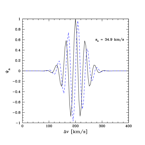
In configuration space this filter is simply a plane-wave, damped by a Gaussian. In Fourier space, the filter is a Gaussian centered around $k=k_{0}$. We would like the filter to have zero mean. Throughout this work we choose $k_{0}s_{n}=6$, in which case Equation 3 shows that the zero mode of the filter $\Psi_{n}(k=0)$ is extremely close to zero, satisfying closely the zero mean requirement. This filter clearly has the properties of being localized in both configuration space and Fourier space. These are among the defining properties of a ‘wavelet filter’, and the filter of Equations (2) and (3) is known as a ‘Morlet Wavelet’ in the wavelet literature. We plot its form in Figure 1 for $s_{n}=34.9$ km/s, which, as we discuss further below, turns out to be one convenient choice. Note that the filters $\Psi_{n}$ (Equation 2) do not form an orthogonal set, but this is unnecessary for our present purposes. We do not expand the entire spectrum in terms of a wavelet basis in this work – the Morlet wavelet, with locality in real and configuration space, is simply a convenient filter.

We then convolve each observed (or simulated) spectrum with the above filter. In this paper, we consider throughout the fractional Ly-$\alpha$ transmission field, $\delta_{F}=(F-\langle F\rangle)/\langle F\rangle$. Here $F=e^{-\tau}$ is the Ly-$\alpha$ transmission, and $\langle F\rangle$ is the global average Ly-$\alpha$ transmission. We label the flux field, $\delta_{F}$, convolved with the filter $\Psi_{n}$ as $a_{n}$:

$$a_{n}(x)=\int dx^{\prime}\Psi_{n}(x-x^{\prime})\delta_{F}(x^{\prime}),$$ (4)

and compute the convolution using Fast Fourier Transforms (FFTs). Note that $a_{n}(x)$ is a complex number for our choice of filter, $\Psi_{n}(x)$. A measure of small-scale power is then

$$A(x)=|a_{n}(x)|^{2},$$ (5)

which for brevity of notation we sometimes refer to as ‘the wavelet-filtered field’ or as ‘the wavelet amplitudes’ (even though it is proportional to the transmission field squared). It is also useful to note that the average wavelet amplitude is just

$$\langle|a_{n}(x)|^{2}\rangle=\int_{-\infty}^{\infty}\frac{dk^{\prime}}{2\pi}\left[\Psi_{n}(k^{\prime})\right]^{2}P_{F}(k^{\prime}),$$ (6)

with $P_{F}(k)$ denoting the power spectrum of $\delta_{F}$. Hence, the mean wavelet amplitude is nothing more than the usual flux power spectrum for some convenient ‘band’ of wavenumbers (see Figure 5 for further illustration). Additional statistics of $A(x)$, beyond the mean, characterize the spatial variations in the small-scale transmission power.

We frequently find it convenient to smooth $A(x)$ using a top-hat filter of smoothing length $L$:

$$A_{L}(x)=\frac{1}{L}\int_{-\infty}^{\infty}dx^{\prime}\Theta(|x-x^{\prime}|;L/2)A(x^{\prime}).$$ (7)

Here $\Theta(|x-x^{\prime}|;L/2)=1$ for $|x-x^{\prime}|\leq L/2$ and is zero otherwise. Smoothing the wavelet filtered field is desirable since the small-scale power is not a perfect indicator of the local temperature, and smoothing reduces the noisy excursions that the wavelet amplitudes can take. Since the hot regions are expected to be rather large during HeII reionization (McQuinn et al. 2008), we can smooth considerably without diluting any temperature inhomogeneities. We generally adopt $L=1,000$ km/s, corresponding to roughly $\sim 10$ co-moving Mpc/$h$ at $z=3$. We discuss this choice further below.

Figure 2.— Illustration of our filtering method. Top panel: A simulated spectrum, with some portions of the spectrum drawn from a simulated ‘hot’ model with $T_{0}=2\times 10^{4}$ K and $\gamma=1.3$, and other regions drawn from a ‘cold’ model with $T_{0}=1\times 10^{4}$ K and $\gamma=1.3$. The hot and cold regions are alternating and are each of length $20$ co-moving Mpc/$h$ ($2230$ km/s). Bottom panel: The red dashed lines and the tick marks on the right hand side of the panel indicate the temperature of the corresponding regions in the upper panel. The solid blue line shows the wavelet-amplitudes (for $s_{n}=34.9$ km/s), top-hat filtered with a $L=1,000$ km/s filter. The smoothed wavelet amplitudes are a good tracer of the temperature of each region.

.

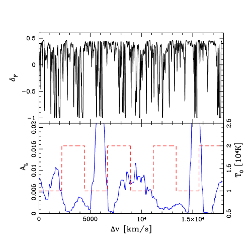
Since thermal broadening smooths the optical depth field on tens of km/s scales, $A_{L}(x)$ should be a good tracer of the temperature for suitable choices of $s_{n}$. In order to illustrate this concretely, we apply the filter to a simulated spectrum from a simple toy inhomogeneous temperature model, following a similar example from Theuns & Zaroubi (2000). Specifically, we splice together simulated lines of sight (see §4.1) with alternating portions of spectrum drawn from each of a ‘hot’ temperature model with $T_{0}=2\times 10^{4}$ K, and $\gamma=1.3$, and a ‘cold’ temperature model with $T_{0}=1\times 10^{4}$ K, and $\gamma=1.3$. We refer the reader to §4.1 and §Appendix C: Convergence with Simulation Resolution and Boxsize for details regarding the simulated spectra. If the wavelet filtered field provides a good indicator of the temperature, regions with hot temperatures should tend to produce low wavelet amplitudes, while the cold regions should produce high wavelet amplitudes. The results of this test are shown in Figure 2, for smoothing scales of $s_{n}=34.9$ km/s and $L=1,000$ km/s. Cold regions tend to contain several narrow lines, and produce a large response after filtering: the regions near $\Delta v=6,000$ km/s and $15,000$ km/s have $A_{L}\gtrsim 0.02$. The hot regions typically have $A_{L}\lesssim 0.005$ and never reach the large amplitudes found in the cold regions. There is some variance in the wavelet amplitude from region to region – for example, $A_{L}$ is not as large in the cold region near $\Delta v=10,000$ km/s as it is at $\Delta v=6,000$ km/s and $15,000$ km/s. Nonetheless, the smoothed wavelet amplitude is a fairly good tracer of the underlying temperature field.

Figure 3.— PDF of the wavelet amplitudes for different models at $z=3$ and $s_{n}=34.9$ km/s. The curves show simulated models for the PDF of the wavelet amplitudes, top-hat smoothed over $L=1,000$ km/s, for several temperature-density relations. The mean transmitted flux is fixed in this comparison. The black solid and red-dashed curves correspond very roughly to temperature-density relations expected just after HeII reionization. The blue short-dashed and green long-dashed curves, on the other hand, loosely correspond to the temperature-density relation expected when HI and HeII are both reionized much before $z=3$.

Figure 4.— PDF of the wavelet amplitudes for different models at $z=3$ and $s_{n}=69.7$ km/s. Similar to Figure 3, except for $s_{n}=69.7$ km/s.

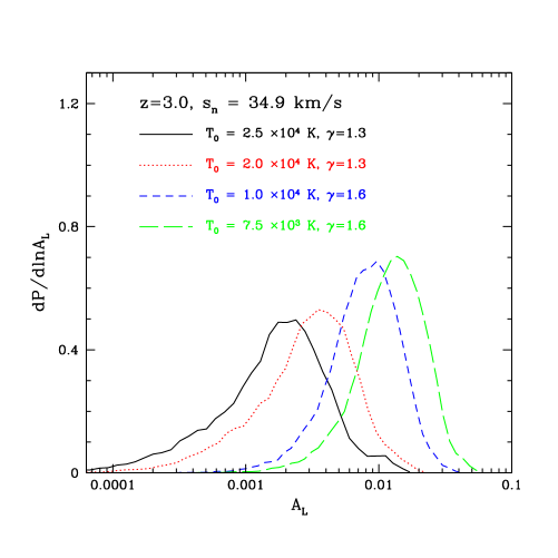
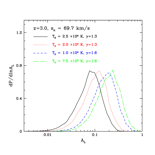
In order to quantify this further, we calculate the probability distribution function (PDF) of the smoothed wavelet amplitudes. We do this for the two choices of small-scale smoothing adopted in this paper (see §2.3): $s_{n}=34.9$ km/s, and twice this, $s_{n}=69.7$ km/s. The PDF of smoothed wavelet amplitudes will be the main statistic we consider in the present paper. For now, we examine models with homogeneous temperature-density relations. The models we select for the temperature-density relation loosely correspond respectively to what one expects right after HeII reionization ($T_{0}\sim 20-25,000$ K and $\gamma=1.3$) (McQuinn et al. 2008), and to what one expects if HI, HeI, and HeII are all ionized much before $z\sim 3$ ($T_{0}\sim 7,500-10,000$ K and $\gamma=1.6$) (Hui & Haiman 2003). The latter, cooler model, might be expected if, for example, the IGM is reionized by abundant faint quasars which have sufficiently hard spectra to doubly ionize helium at the same time they reionize hydrogen, or if high redshift galaxies have a surprisingly hard spectrum and can doubly ionize helium themselves. Note that the precise $z\sim 3$ temperature in the early reionization models is determined by residual photoheating and depends on the reprocessed spectra of the post-reionization ionizing sources (Hui & Haiman 2003).

The PDFs in these models are shown for two choices of small-scale smoothing in Figure 3 ($s_{n}=34.9$ km/s), and Figure 4 ($s_{n}=69.7$ km/s). A larger range of models will be examined in §4. Considering first the smaller smoothing scale (Figure 3), one sees that the peak of the PDF in the $T_{0}=20,000$ K, $\gamma=1.3$ model is reached at a smoothed wavelet amplitude that is roughly a factor of $2$ smaller than the peak location in the $T_{0}=10,0000$ K, $\gamma=1.6$ model. The PDFs in the hotter $T_{0}\sim 25,000$ K model and the colder $T_{0}=7,500$ K model differ by even more. In the midst of HeII reionization, one expects an inhomogeneous temperature field and the true temperature-density relation may be a mix of the models shown here. At any rate, the wavelet PDFs differ significantly in the models with $20,000$ K and those with cooler temperatures. This further demonstrates – beyond the visual inspection of Figure 2 – that the wavelet PDF is a useful statistic for constraining the thermal history and HeII reionization. The typical wavelet amplitude in each model is significantly larger at $s_{n}=69.7$ km/s (Figure 4), a consequence of the roughly exponential fall-off in flux power towards high $k$ (Zaldarriaga et al. 2001). The PDFs still vary significantly with temperature-density relation at this larger smoothing scale, although the sensitivity is a little bit reduced.

2.3. Smoothing Scales

Figure 5.— Relation between the mean wavelet amplitude and flux power spectrum. The red solid and blue dashed lines show the usual flux power spectrum for simulated models with two different temperature-density relations at $z=3$, with the mean transmitted flux fixed at $\langle F\rangle=0.680$ for each model. The black dashed vertical lines indicate the range of scales ($\pm 1-\sigma$) extracted by the $s_{n}=69.7$ km/s wavelet filter, while the blue dotted vertical lines indicate the same for the $s_{n}=34.9$ km/s filter.

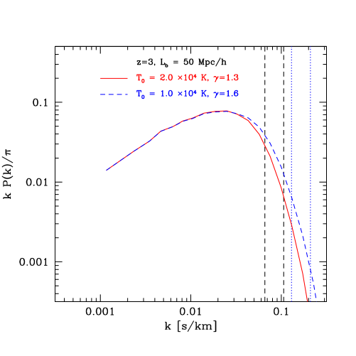
Before we move on to analyze observational data, let us consider further the two smoothing scales, $s_{n}$ and $L$, in our calculations. We make measurements for two choices of small-scale smoothing: $s_{n}=34.9$ km/s and $s_{n}=69.7$ km/s. For the former choice of smoothing scale $|\Psi_{n}(k)|^{2}$ is proportional to a Gaussian centered on $k_{0}=6/s_{n}=0.17$ s/km, with width $\sigma_{k}=\sqrt{2}/s_{n}=0.04$ s/km. The latter choice of smoothing scale centers the Gaussian on $k_{0}=6/s_{n}=0.086$ s/km, with a width of $\sigma_{k}=\sqrt{2}/s_{n}=0.02$ s/km. The range of scales probed by these filters is shown in comparison to simulated flux power spectra in Figure 5. As illustrated in Figures 3, 4, and 5, the wavelet PDFs are slightly less sensitive to the IGM temperature for the larger smoothing scale filter. On the other hand, the results at the larger smoothing scale are less sensitive to metal line contamination and other systematics. Increasing the smoothing by still another factor of two would almost completely remove the sensitivity to temperature (see Figure 5). Decreasing $s_{n}$ by an additional factor of two (to $s_{n}=17.4$ km/s) increases the fractional difference between model curves, but brings one very far out on the exponential tail of the power spectrum (Figure 5) and makes the results very sensitive to metal line contamination, detector noise, and pixelization effects. The two choices of filtering scale used here represent a compromise between discriminating power and systematic effects. Considering both choices of filtering scale gives a consistency check on the results and helps to protect against systematic effects.

Let us now consider the large scale smoothing, $L$. Naively, one would want to tune this filtering to precisely the scale on which the temperature field is inhomogeneous. Since the power spectrum of temperature fluctuations during HeII reionization has a relatively well defined peak (McQuinn et al. 2008), one might expect the variance of the wavelet amplitudes to also show a clear maximum at some characteristic smoothing scale. However, in practice we find that this is washed out in Ly-$\alpha$ forest spectra, which as one dimensional skewers suffer owing to aliasing from high-$k$ modes transverse to the line of sight (Kaiser & Peacock 1991). To illustrate this, consider the two-point function of the wavelet amplitudes (squared),

$$\xi_{A}(|v_{1}-v_{2}|)=\frac{\langle A(v_{1})A(v_{2})\rangle-\langle A\rangle^{2}}{\langle A\rangle^{2}},$$ (8)

and its Fourier transform, the power spectrum of wavelet-amplitudes squared, $P_{A}(k)$. Here $v_{1}$ and $v_{2}$ are two points along a quasar spectrum and $\langle A\rangle$ is the globally averaged wavelet amplitude squared, and we have normalized this two-point function by the (square of the) mean wavelet amplitude squared. The power spectrum of wavelet amplitude squared fluctuations encodes how much the small-scale power spectrum fluctuates across a quasar spectrum as a function of scale. It involves a product of four values of $\delta_{F}$ and is hence a four-point function.

Figure 6.— Power spectra of the squared wavelet amplitudes. The curves show power spectra for two different (homogeneous temperature-density relation) models. Aside from the small-scale turn-over, which owes to the smoothing (on scale $s_{n}=34.9$ km/s) from the wavelet filter, the model curves are quite flat as a function of wavenumber.

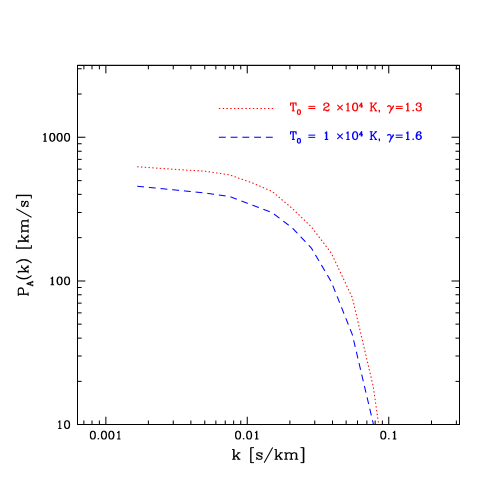
We show two simulated examples of $P_{A}(k)$ in Figure 6 for $s_{n}=34.9$ km/s. One can see that, except for the small-scale cut-off, the power spectra are quite flat as a function of scale. This is somewhat unfortunate, as one would naively hope that the scale dependence of $P_{A}(k)$ would directly reveal the scale dependence of temperature fluctuations, but the flatness we find is a direct consequence of aliasing. We have experimented with various inhomogeneous temperature models, including simulated models from McQuinn et al. (2008) and find similarly flat power spectra. One might be able to get around this by using quasar pairs to measure the power spectrum of wavelet amplitude squared transverse to the line of sight. We defer, however, investigating this to future work. For the moment, our main conclusion is that, owing to the flatness of $P_{A}(k)$, the precise smoothing scale $L$ is relatively unimportant. Hence we generally stick to $L=1,000$ km/s as a convenient choice. We nevertheless investigate the dependence on large scale smoothing from observational and simulated data in §4.4.

To summarize, by applying a very simple filter to a quasar spectrum, we can measure the small-scale power spectrum of transmission fluctuations as a function of position across each spectrum, and thereby constrain the temperature of the IGM. Note that our procedure does not involve identifying absorption lines and fitting profiles to identified lines, (although we find in §3 that it is important to identify metal absorbers in the forest which does involve line-fitting). It is instead within the spirit of treating the forest as a one dimensional random field and measuring the statistics of this continuous field (e.g. Croft et al. 1998). This is more appropriate given the modern understanding that the forest arises from fluctuations in the line of sight density field, rather than discrete absorbing clouds (e.g. Hernquist et al. 1996, Miralda-Escudé et al. 1996, Katz et al. 1996). In this way our approach is very similar to Theuns & Zaroubi (2000) and Zaldarriaga (2002), and somewhat resembles Zaldarriaga et al. (2001), but is rather different than Schaye et al. (2000), Ricotti et al. (2000) and McDonald et al. (2001).

Additionally, recall that the widths of most of the absorption lines in the Ly-$\alpha$ forest are dominated by the Hubble expansion across an absorber, and not by thermal broadening (Hernquist et al. 1996, Weinberg et al. 1998). In order to determine the temperature with a line fitting method, one typically looks for a low-end cut-off in the distribution of line widths (e.g. Schaye et al. 2000). One might worry that this throws out information as thermal broadening smooths the spectrum everywhere. In practice, though, it appears that most of the signal and information in our method also arises from deep narrow lines which produce a large response after wavelet filtering. Another possible issue is that the precise interpretation of the line width cut-off in the line-fitting studies is unclear when the temperature field is inhomogeneous. It would certainly be interesting to compare more closely the different methods, but we defer this to future work. For now, note that our method is very simple to apply.

3. Data Analysis

We now move on to apply the method to observational data. The main result will be a measurement of the PDF of the smoothed wavelet amplitudes at $z\sim 2.2-4.2$. Our data set consists of $40$ quasar spectra observed with UVES on the VLT, described and reduced as in Dall’Aglio et al. (2008). We have identified metal lines in the Ly-$\alpha$ forest for $11$ of these spectra, as described in §3.2. The spectra have high $S/N$ ranging from $S/N\sim 30-130$ (quoted at the continuum level per $0.05\AA$ pixel), and high spectral resolution, $\rm{FWHM}\sim 6$ km/s. High spectral resolution and $S/N$ are essential to reliably probe high-$k$ modes in the spectra and to estimate the temperature of absorbing gas. A detailed list of the quasar spectra, with redshift estimates and other properties, can be found in Dall’Aglio et al. (2008).

3.1. Raw Measurements

We aim to estimate the small-scale power in a way that minimizes sensitivity to uncertainties in the quasar continuum. Dall’Aglio et al. (2008) carefully continuum fit the data we use here, and used Monte Carlo simulations to check the accuracy of their fits. We can further mitigate uncertainties by considering fluctuations in the transmission around the mean, relative to the mean. This is helpful because the overall normalization of the continuum divides out. Provided that the continuum varies slowly across each spectrum in comparison with the fluctuations in the forest, we can additionally remove any slowly varying trend produced by the quasar continuum – or any slowly-varying residuals in the case of data that has previously been continuum fitted – and obtain an unbiased estimate of the small-scale structure in the forest (Hui et al. 2001). For each spectrum, we estimate a running mean flux by filtering the data on large scales as in Croft et al. (2002), Kim et al. (2004), and Lidz et al. (2006). Our estimate of the fractional transmission is then:

$$\hat{\delta}_{F}(\Delta v)=\frac{F(\Delta v)-F_{R}(\Delta v)}{F_{R}(\Delta v)}.$$ (9)

Here $F(\Delta v)$ is the flux at velocity separation $\Delta v$, and $F_{R}(\Delta v)$ is the spectrum smoothed with a large radius filter. We use here a Gaussian filter with radius $R=2,500$ km/s. One may form $\hat{\delta}_{F}$ using either the raw flux or a continuum-normalized flux. In the present work, we use the continuum fitted data from Dall’Aglio et al. (2008) throughout. The large scale filter removes any slowly-varying trend owing to structure in the underlying quasar continuum from, e.g. weak emission lines, or slowly varying residuals in the case of continuum fitted data. It also means that we sacrifice measuring large scale modes in the Ly-$\alpha$ forest, but we presently focus on small-scale structure, and sufficiently large scale modes are regardless dominated by structure in the quasar continuum. We refer the reader to Croft et al. (2002) and Lidz et al. (2006) for some tests illustrating the robustness of $\hat{\delta}_{F}$ to continuum-fitting uncertainties. As a double-check that the present results are insensitive to the precise $\hat{\delta}_{F}$ estimator, we also generated $\hat{\delta}_{F}$ with a different choice of large scale smoothing for one of our redshift bins, $R=10,000$ km/s – i.e., close to the flat mean case – and found a nearly identical wavelet PDF.

We begin by estimating $\hat{\delta}_{F}$ across each spectrum, first re-binning, using linear interpolation, all of the data onto uniform pixels in velocity space with $\Delta u=4.4$ km/s. We consistently use the same binning in constructing simulated spectra. This avoids effects from variable pixelization, while still preserving the scales of interest. After forming $\hat{\delta}_{F}$ across each spectrum, we break the data into several (contiguous and non-overlapping) redshift bins of full-width $\Delta z=0.4$, centered around $\bar{z}=2.2,2.6,3.0,3.4,3.8$, and $4.2$. Owing to uneven redshift sampling in the data set, the redshift bin at $\bar{z}=3.8$ (Dall’Aglio et al. 2008) would be almost entirely empty and so we do not consider it further here. This occurs because most of the spectra in the Dall’Aglio et al. (2008) sample have emission redshift $z_{\rm em}\lesssim 3.7$, but the sample has two high quality spectra at emission redshift above $z_{\rm em}\gtrsim 4.6$, which contribute extended ($\gtrsim 150$ co-moving Mpc) stretches to our highest redshift bin at $\bar{z}=4.2$. We select only spectral regions that lie between rest frame wavelengths of $\lambda_{r}=1050$ $\AA$ and $\lambda_{r}=1190$ $\AA$. This conservative cut serves to remove spectral regions that may be contaminated by either the proximity effect, by the Ly-$\beta$ forest (and other higher Lyman series lines), or by Ly-$\beta$ and OVI emission features. We then form the wavelet amplitude squared field, smoothed at $L=1,000$ km/s, using Equations 2 – 7. The resulting spectra and wavelet amplitudes are visually inspected. Regions impacted by DLAs, or with obvious spurious stretches, are removed from the data sample by hand.

Figure 7.— Example spectrum and smoothed wavelet amplitudes from the $\bar{z}=2.2$ bin. Top panel: The fractional transmission fluctuations $\hat{\delta}_{F}$ for the spectrum of the quasar HE1158-1843. Middle panel: The amplitude squared of the wavelet filtered field, formed with a $s_{n}=34.9$ km/s filter, smoothed over $L=1,000$ km/s. Bottom panel: Similar to the middle panel, but using a Morlet wavelet with $s_{n}=69.7$ km/s. Note that the y-axis in the bottom two panels have rather different ranges. This is required because of the strong dependence of small scale power on smoothing scale.

Figure 8.— Example spectrum and smoothed wavelet amplitudes from the $\bar{z}=2.6$ bin. Similar to Figure 7, but for the spectrum of HE2243-6031. Note that the x and y axes have different ranges than in the previous figure. The x-axis range is set by the portion of the forest that we use from the example spectrum in a given redshift bin. We vary the y-axis range because the mean wavelet amplitude changes strongly with redshift, owing mostly to evolution in the mean absorption, and so a varying range is necessary for visual clarity.

Figure 9.— Example spectrum and smoothed wavelet amplitudes from the $\bar{z}=3.0$ bin. Similar to Figure 7, but for the spectrum of Q2139-4434. Note that the x and y axes have different ranges than in the previous figures.

Figure 10.— Example spectrum and smoothed wavelet amplitudes from the $\bar{z}=4.2$ bin. Similar to Figure 7, but for the spectrum of BR1202-0725. Note that the x and y axes have different ranges than in the previous figures.

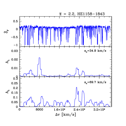
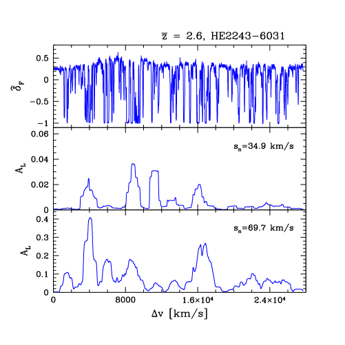
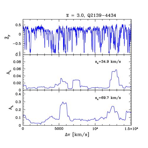
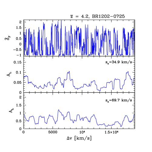
It is instructive to examine a few example spectra visually before measuring their detailed statistical properties. In Figures 7 – 10 we show several spectra, along with the corresponding (smoothed) wavelet amplitudes squared for a few redshift bins. The most conspicuous change across the different redshift bins is the increasing average absorption with increasing redshift. Since we are considering fractional fluctuations, this manifests itself as an increase in the fraction of pixels with $\hat{\delta}_{F}$ close to $-1$, with occasional excursions to very large $\hat{\delta}_{F}$. The next impression provided by the spectra appears at first tantalizing: most regions have low $A_{L}$, but there are occasional upward excursions over portions of the spectrum. This behavior is especially apparent for the smaller of the two filtering scales, and is less apparent in the highest redshift case (Figure 10).

Consider for example the spectrum Q2139-44, in the $\bar{z}=3.0$ bin, convolved with a $s_{n}=34.9$ km/s Morlet filter, as shown in Figure 9. In this spectrum the regions near $\Delta v=5,000$, $7,500$, and $12,500$ km/s all have relatively high wavelet amplitudes, $A_{L}\gtrsim 0.02$, while the rest of the spectral regions have low amplitude. Inspecting the simulated PDF of Figure 3, the low amplitude floor with $A_{L}\sim 0.005$ seems to indicate hot $T_{0}\sim 20,000$ K gas, while the regions with $A_{L}\gtrsim 0.02$ seem to require cooler gas $T_{0}\lesssim 7,500$ K gas.

Figure 11.— Example wavelet amplitude field compared with models. The smoothing scale is $s_{n}=34.9$ km/s here. The blue lines are the same as in Figure 9. The observed wavelet amplitudes are shown by a dashed line to avoid confusion with the model curves. The red and black lines in the bottom panel are simulated sightlines for a hot IGM model (red), and a cold IGM model (black). Random noise has been added to the simulated spectra (see §4.5). The wavelet amplitudes in most spectral regions are roughly consistent with the hot IGM model, but the high wavelet amplitude excursions (near $\Delta v=5,000$, $7,500$, and $12,500$ km/s) look naively like cold gas. In §3.2, we show that these apparent cold regions are spurious and are instead consistent with being hotter gas contaminated by metal lines.

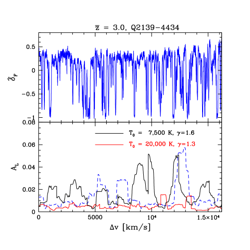
At first glance, these upward wavelet amplitude excursions seem to be cold regions embedded in an otherwise hot IGM. This is what one naively expects in the midst of HeII reionization: cool regions where HI and HeI reionized long ago, and hotter regions where helium is doubly ionized. Before we dispel this fantasy – these regions are contaminated by metal absorbers (see §3.2) – let us add some sightlines from simulated models to further illustrate this (Figure 11). The sightlines show that the low wavelet amplitude floor in the observed spectrum roughly matches the hot IGM sightline. This implies that there are indeed significant quantities of hot $\sim 20,000$ K gas in the IGM at $z=3$. However, the hot model fails to produce the high wavelet amplitude excursions seen in the data. Matching these seems, at first glance, to require a cooler model – one with roughly $T_{0}\sim 7,500$ K, $\gamma=1.6$, for example. (To be clear, note that the simulation and observational data are drawn from different realizations, so one does not expect the simulated case to match the observations region-by-region or feature-by-feature. The meaningful comparison is the overall number of regions with high or low wavelet amplitude.) It is at first tempting to conclude that we are detecting temperature inhomogeneities from incomplete HeII reionization.

3.2. Metal Line Contamination

We need, however, to consider a very important systematic. A hot region that lands at the same wavelengths as a ‘clump’ of prominent narrow metal lines may look to us like a cold region. The wavelet filter just tells us the total level of small-scale power from place to place, and does not distinguish whether absorption arises from HI or some other element. To make a robust estimate of the IGM temperature, we need to identify metal line absorbers within the Ly-$\alpha$ forest. We expect metal line contamination to be most severe in the low redshift bins, where the fractional contribution of metals to the overall opacity in the forest is highest (e.g. Faucher-Giguère et al. 2008b), and on the smaller of our two filtering scales (see Appendix B).

Naturally, distinguishing metal absorption lines and Ly-$\alpha$ lines within the Ly-$\alpha$ forest is a challenging and imperfect process. We do, however, have a few separate handles on distinguishing metal lines from Ly-$\alpha$ lines within the forest. First, we identify all of the metal absorbers redward of Ly-$\alpha$ and look for ‘partner’ transitions. The partner transitions are additional transitions that lie at the same redshift as an identified red-side line, yet which land within the Ly-$\alpha$ forest. Next, we search for doublets within the Ly-$\alpha$ forest, which can be identified by their distinctive optical depth ratios and by the characteristic separation between a doublet’s two components. For instance, CIV is a doublet with a strong component at $\lambda_{r}=1548.2\AA$, and a weaker component at $\lambda_{r}=1550.8\AA$, and the ratio of the absorption cross sections of the two components is $2$. So CIV should stand out as a doublet with the two components separated by $\sim 640$ km/s, with the lower wavelength line a factor of two stronger than its partner component. MgII is another prominent doublet. After identifying a doublet, one can use the estimated redshift of an identified doublet to search for additional transitions at the same redshift: we look for CII/III/IV, NII/III/V, OI/VI, MgI/II, AlII/III, SiII/III/IV, SVI, and FeII, and consider further transitions for DLAs. This approach already identifies a host of metal lines within the forest, but there are inevitably some remaining metal lines left within the forest. For example, there are sometimes absorbers where the doublet features are undetectable owing to line blending. To further mitigate metal line contamination, our final step is to mark extremely narrow lines (with b-parameter $b\lesssim 7$ km/s) as metals. This final cut amounts to only $25\%$ of the identified lines. Clearly, one needs to be careful about making cuts based on line width: doing so could bias us against detecting cold regions. However, for an HI line to have a linewidth of $b\lesssim 7$ km/s it needs to have an implausibly low temperature of $T\lesssim 3,000$ K. Hence, we are confident that this final cut does not bias our results, yet it helps protect against remaining unidentified metal lines within the forest. We will subsequently present tests to check how much the results depend on the precise way in which we excise metal line contaminated regions.

In this paper, we have identified metal lines for $11$ of the $40$ spectra in our data sample. The identified metals come entirely from portions of spectrum absorbing at $z\lesssim 3$ – where we expect the metal line contamination to be strongest – and not in the higher redshift bins. That is, we do not presently have estimates of metal line contamination in the redshift bins centered around $\bar{z}=3.4$ and $\bar{z}=4.2$. In these redshift bins, we will focus entirely on the larger ($s_{n}=69.7$ km/s) filtering scale where the metal line contamination is less of an issue (Appendix B).

In order to check the influence of metal line contamination, we calculate the wavelet amplitudes as before, and excise regions impacted by metal line contamination. An important assumption here is that gas absorbing in a metal line transition at a given wavelength is spatially uncorrelated with gas absorbing in Ly-$\alpha$ at nearby wavelengths. If this assumption were violated, we could bias ourselves by preferentially removing regions of above average hydrogen absorption when excising metal contaminated regions. Fortunately, most of the metal line transitions have rest-frame wavelengths that are very different than that of Ly-$\alpha$ and so the gas absorbing in a metal transition at a given wavelength is very widely separated (in physical space) from that absorbing in Ly-$\alpha$. Hence the metal and Ly-$\alpha$ absorption are uncorrelated. This justifies our approach. Since the wavelet filter is not completely local, pixels with metal line absorption will contaminate neighboring pixels after filtering. Furthermore, we generally smooth the wavelet squared field over $L=1,000$ km/s. As a simple and conservative cut, we examine the fraction of contaminated pixels within a smoothing length $L$ around each pixel, and discard a pixel if less than $f_{m}=95\%$ of its neighbors (within a smoothing length) are metal free.

Figure 12.— Example of the impact of metal line contamination from the $\bar{z}=2.2$ bin. Identical to Figure 7, except illustrating the impact of metal line contamination. Top panel: Red lines, and short black dashed lines above the spectrum, indicate identified metal lines within the Ly-$\alpha$ forest. Middle panel: The short black lines identify the centers of pixels with identified metal lines. The red lines indicate the approximate regions where metal lines impact the wavelet amplitudes (for $f_{m}=0.95$, see text). Most of the wavelet amplitude peaks correspond to metal line contaminated regions for this filtering scale ($s_{n}=34.9$ km/s). Bottom panel: Similar to the middle panel, for $s_{n}=69.7$ km/s.

Figure 13.— Example of the impact of metal line contamination from the $\bar{z}=2.6$ bin. Similar to Figure 12 but for the spectrum HE0940-1050 in the $\bar{z}=2.6$ bin. Notice in particular that the very large wavelet amplitudes near $\Delta v=2,000$ km/s for $s_{n}=34.9$ km/s correspond closely to several strong metal lines. Again the wavelet peaks at this filtering scale trace mostly metal line contaminated regions. The lower wavelet amplitude regions, and not these high amplitude portions, indicate the IGM temperature. Note that the metal line contamination is less severe for the larger smoothing scale filter in the bottom panel.

Figure 14.— Example of the impact of metal line contamination from the $\bar{z}=3.0$ bin. Similar to Figure 12 and Figure 13, but for the portion of HE0940-1050 in the $\bar{z}=3.0$ bin. Once again the large wavelet amplitude regions at filtering scale $s_{n}=34.9$ km/s are metal contaminated.

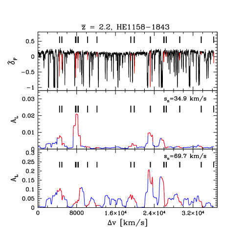
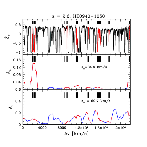
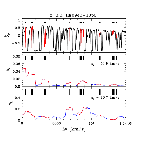
We find that metal line contamination can have a significant impact, especially for $s_{n}=34.9$ km/s, and at $z\lesssim 3$. We show a few example sightlines in Figures 12 – 14. It is striking that the most prominent peaks in the wavelet filtered field at $s_{n}=34.9$ km/s, shown in the figures, correspond very closely to metal lines. Essentially, our filter was designed to look for temperature inhomogeneities, but it appears most effective at identifying metal-line contaminated regions! In fact, wavelet filtering may be a good way to quickly identify prominent metals in the forest. The metal line contamination is less severe for spectra passed through the larger wavelet filter ($s_{n}=69.7$ km/s). The amplitude of fluctuations in the forest is much greater on this smoothing scale. The metals also generally contribute more power on the larger smoothing scale, but the amplitude of fluctuations from HI increases more strongly with smoothing scale, and so the metals are fractionally less important on larger scales. This is perhaps seen most easily in the example of Figure 13. In the $s_{n}=34.9$ km/s panel of this figure, all of the prominent peaks are metal contaminated regions. In the larger smoothing scale panel, there are some peaks from HI and some from metals, and the heights of the various peaks are comparable. The more significant contamination of the metals on the smaller smoothing scale likely results because the metal lines tend to be narrower than the HI lines. In Appendix B we find qualitatively similar results by adding metal line absorbers, with empirically derived properties, to mock Ly-$\alpha$ forest spectra.

Since we can attribute many of the peaks observed in the wavelet amplitudes to metal lines, this does imply, however, that the temperature inhomogeneities cannot be too large. If temperature inhomogeneities were present and large, we would expect to see more high wavelet amplitude regions left over after excising the metals. In particular, consider Figure 11. In this example, we found that the low wavelet amplitude regions of the spectrum are consistent with hot $20,000$ K gas. While we have not identified metal lines for this particular spectrum, our results from other lines of sight clearly suggest that the high wavelet amplitude regions are metal-contaminated rather than genuine cold regions with $T_{0}\sim 7,500-10,000$ K. The lack of high wavelet amplitude regions after metal excision implies there are few such cold regions left, and that most of the volume of the IGM at $z\sim 3$ is hot with $T_{0}\sim 20,000$ K (although see §4.1 for a discussion regarding the dependence of our results on $\gamma$).

It is clear, however, that metal line contamination is a very important systematic for these measurements, although the contamination is less of an issue on the larger smoothing scale and for the high redshift measurements. This issue is not unique to our method, although the detailed impact of metal lines will depend on the precise algorithm for constraining the IGM temperature. For instance, measurements based on fitting the minimum width of absorption lines in the Ly-$\alpha$ forest need to carefully avoid including metal lines in the sample of lines used to estimate the temperature. Power spectrum based temperature estimates need to account for the small-scale power contributed by metal absorbers or mask the metal absorbers before estimating the power spectrum.

3.3. The Wavelet Amplitude Squared PDF

Let us now move past mere visual inspection and measure statistical properties from the observed spectra. We focus mostly on the PDF of $A_{L}$ for our fiducial choices of $s_{n}=34.9$ km/s, $s_{n}=69.7$ km/s, $L=1,000$ km/s, and $f_{m}=0.95$. In each redshift bin, we find the minimum and maximum $A_{L}$ and then choose $10$ evenly-spaced logarithmic bins in $A_{L}$ for the PDF measurement. We tabulate the average $A_{L}$ and the differential PDF in each $A_{L}$ bin for each redshift bin. The average redshift of pixels in a redshift bin is typically close to the redshift at bin center, and the error bars are still fairly large, so we ignore any issues associated with redshift evolution across each bin and quote all results at the bin center.

We use a jackknife resampling technique to calculate error bars for the PDF measurements. We first estimate the PDF from the entire data sample within a given redshift bin, $\hat{P}(A_{i})$. Here $\hat{P}(A_{i})$ is the PDF estimate for the ith $A_{L}$ bin, and $A_{i}$ is the average wavelet amplitude squared and smoothed within the bin. Next we divide the data set into $n_{g}=10$ subgroups, and estimate the PDF of the data sample omitting each subgroup. Let $\tilde{P}_{k}(A_{i})$ represent the PDF estimate omitting the pixels in the kth subgroup. Then our estimate of the jackknife covariance between bins $i$ and $j$, $C(i,j)$, is:

$$C(i,j)=\sum_{k=1}^{n_{g}}\left[\hat{P}(A_{i})-\tilde{P}_{k}(A_{i})\right]\left[\hat{P}(A_{j})-\tilde{P}_{k}(A_{j})\right].$$

(10)

In practice our estimates of the off-diagonal elements of the covariance matrix are very noisy. Consequently, we will be forced to ignore the off-diagonal elements of $C(i,j)$. We have tested the jackknife error estimator with lognormal mocks (see McDonald et al. 2006, Lidz et al. 2006) that approximately mimic the properties of the current data set. We generate $10,000$ mock realizations of a $z=3$ data set and compare error bars estimated from the dispersion across the mock realizations with the jackknife error estimates. In the mock data, we find that neglecting the off-diagonal elements in the covariance matrix increases the average value of $\chi^{2}$ by $\sim 1$ for $14$ degrees of freedom (the mock PDFs had $15$ rather than $10$ $A_{L}$ bins), and so ignoring the off-diagonal elements is likely a good approximation. The jackknife estimates of the diagonal elements of the covariance matrix agree with direct estimates of the dispersion across the mock data to better than $20\%$ on average, although the jackknife estimator sometimes under-predicts the errors in the tails of the PDF more severely. We provide tables of the wavelet PDF measurements in Tables 1–5.

3.4. Shot Noise

We plot the measured wavelet PDF in the next section, but pause to consider first the impact of shot-noise. The observed Ly-$\alpha$ forest spectra are contaminated by random noise owing to Poisson fluctuations in the discrete photon count and around the mean night sky background count, as well as by random read-out noise in the CCD detector (see e.g. Hui et al. 2001 for discussion). We need to consider how this noise impacts the wavelet PDF measurements.

In Appendix A, we derive estimates of the noise bias for measurements of the first two moments of the wavelet amplitude PDF. We apply these formulae here to estimate the impact of noise on the present measurements. On the larger smoothing scale, $s_{n}=69.7$ km/s, we find that shot-noise bias is unimportant for our present data set. For example, at $z=3$, applying the formulae of Appendix A, we find that the noise contamination to the mean wavelet amplitude is less than one-third of the 1-$\sigma$ statistical error on this quantity for our present data sample. Similarly, in this redshift bin and for this smoothing scale, we find that the wavelet amplitude variance is biased by random noise only at the $\sim 1\%$ level. However, the shot-noise bias is not negligible on the smaller smoothing scale, $s_{n}=34.9$ km/s. For instance, a quasar spectrum with $S/N\sim 50$ at the continuum contributes a mean wavelet amplitude owing to noise of $\langle|a_{n}^{\rm noise}|^{2}\rangle\sim(N/S)^{2}/\langle F\rangle\sim 6\times 10^{-4}$ at $z\sim 3$ (Appendix A, Hui et al. 2001). This is comparable to the wavelet amplitude signal in the tail of the PDF in the favored hot IGM models (see Figure 3). The more significant noise contamination on the smaller smoothing scale owes to the rapid decline in signal power towards small scales. To guard against noise bias at the smaller smoothing scale, we cut spectra with $S/N\leq 50$ redward of Ly-$\alpha$ from the sample used in the smaller smoothing scale measurement. We cut based on the red side noise, rather than using a noise estimate in the forest, to avoid introducing any possible selection bias. Further, we add noise to the mock spectra when comparing with the measurement on the smaller smoothing scale (§4.5).

4. Theoretical Interpretation

In this section, we compare the wavelet PDF measurements with cosmological simulations in order to estimate the implied IGM temperature. A particular goal here is to determine whether the IGM is closer to the thermal state expected in the midst of HeII reionization ($T_{0}\sim 20-25,000$ K, $\gamma=1.3$) or whether it more closely resembles the state much after a reionization event ($T_{0}\sim 7,500-10,000$ K, $\gamma=1.6$). Furthermore, we aim to check whether the data indicate large temperature inhomogeneities. We perform this comparison over the full redshift range of our data set, $\bar{z}=2.2-4.2$.

4.1. Cosmological Simulations

For the purpose of this project and related Ly-$\alpha$ forest work, we have run a new suite of cosmological smoothed particle hydrodynamics (SPH) simulations using the simulation code Gadget-2 (Springel 2005). The simulations adopt a LCDM cosmology parameterized by: $n_{s}=1$, $\sigma_{8}=0.82$, $\Omega_{m}=0.28$, $\Omega_{\Lambda}=0.72$, $\Omega_{b}=0.046$, and $h=0.7$ (all symbols have their usual meanings), consistent with the WMAP constraints from Komatsu et al. (2009). Each simulation was started from $z=299$, with the initial conditions generated using the Eisenstein & Hu (1999) transfer function. We ran several simulations to test the convergence of our results with boxsize, as well as mass and spatial resolution (see §Appendix C: Convergence with Simulation Resolution and Boxsize). From these tests, we determined that the best choice simulation for the present project has a boxsize of $L_{\rm box}=25$ Mpc/$h$ and $N_{p}=2\times 1024^{3}$ particles, and this run is the fiducial simulation in what follows. This simulation represents a fairly significant improvement in boxsize and resolution compared to most previous work (see §4.10 for details). It has approximately the gas mass recommended for resolution convergence in a recent study by Bolton & Becker (2009), and tracks over an order of magnitude more particles than the simulations of these authors. In each run, the softening length was taken to be $1/20$th of the mean inter-particle spacing. In order to speed up the calculation, we chose an option in Gadget-2 that aggressively turns all gas at density greater than $1000$ times the cosmic mean density into stars (e.g. Viel et al. 2004). Since the forest is insensitive to gas at such high densities, this is a very good approximation.

The simulations were run using the Faucher-Giguère et al. (2009) photoionizing background, which is an update of the Haardt & Madau (1996) model (see, also Katz et al. 1996a, Springel & Hernquist 2003). The ionizing background was turned on at $z=7$ in the simulations. This model for the ionizing background determines the photoheating and gas temperature in the simulation. We would like, however, to explore a wide range of thermal histories. In order to do this, we make an approximation. The approximation is to fix the fiducial ionization history to the Faucher-Giguère et al. (2009) model for the purpose of running the simulation and accounting for gas pressure smoothing, but to vary the temperature-density relation (Equation 1) when constructing simulated spectra. This ‘post-processed spectra’ approximation neglects the dependence of Jeans smoothing on the detailed thermal history of the IGM, but correctly incorporates thermal broadening for a given temperature-density relation model, parametrized by $T_{0}$ and $\gamma$. It also neglects the inhomogeneities in $T_{0}$ and $\gamma$ expected during HeII reionization. Finally, by assuming a perfect temperature-density relation in constructing mock absorption spectra, we also neglect the impact of shock heating – which adds scatter to the temperature density relation (Hui & Gnedin 1997) – on the amount of thermal broadening. We caution against taking the results of these first pass, homogeneous temperature-density relation calculations too literally: if the IGM temperature is significantly inhomogeneous, these calculations provide only a crude approximation. The calculations are meant only to get a sense for whether the IGM is mostly at $T_{0}\sim 20,000$ K, or instead at $T_{0}\sim 10,000$ K, and to check whether large temperature inhomogeneities are present. We intend to make more detailed theoretical calculations in future work.

Although our measurements of the wavelet amplitude PDF are robust to uncertainties in fitting the quasar continuum, our interpretation of the measurements still relies on estimates of the mean transmitted flux. Specifically, we follow the normal procedure of adjusting the intensity of the simulated ionizing background in a post-processing step, so that the simulated mean transmitted flux (averaged over all sightlines) matches the observed mean flux. We assume here the best-fit measurements of Faucher-Giguère et al. (2008b), and subsequently explore the impact of uncertainties in the mean flux (§4.3). We adopt their estimates in $\Delta z=0.2$ bins, and use their measurements that include a correction for metal line opacity based on Schaye et al. (2003), and a continuum-fitting correction (which accounts for the rarity of regions with nearly complete transmission, $F=1$, at high redshift). The corresponding Faucher-Giguère et al. (2008b) measurements in our redshift bins are: $(\bar{z},\langle F\rangle)=(2.2,0.849);(2.6,0.778);(3.0,0.680);(3.4,0.566);$ and $(4.2,0.346)$. We output simulation data at every $\Delta_{z}=0.5$ between $z=4.5$ and $z=2$. In order to generate model wavelet PDFs at redshifts in between two stored snapshots, we measure the simulated wavelet PDF from each stored snapshot and linearly interpolate to find the PDF at the precise desired redshift.

4.2. Comparison with Measurements

Let us first compare the measured PDF in the different redshift bins for $s_{n}=69.7$ km/s. The results of these calculations are shown in Figures 15 – 19. We start with a qualitative ‘chi-by-eye’ assessment, and provide more quantitative constraints in §4.6.

Figure 15.— Comparison between the measured wavelet PDF in the $\bar{z}=4.2$ bin with $s_{n}=69.7$ km/s, $L=1,000$ km/s and simulated models. The blue histogram with points and ($1-\sigma$) error bars is the measured PDF, uncorrected for metal line contamination.

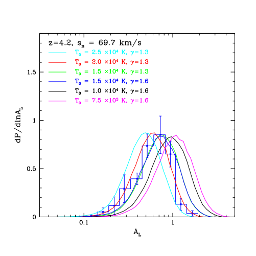
The blue histogram with error bars in Figure 15 shows the measured PDF at $\bar{z}=4.2$, uncorrected for metal line contamination. We have not identified metal lines in the high redshift spectra contributing to this redshift bin, but we expect metal line contamination to have only a small effect on the wavelet PDF at this redshift and smoothing scale (see Appendix B). The model curves with $T_{0}\sim 7,5000-10,000$ K and $\gamma=1.6$ correspond roughly to models in which HI is reionized early, and HeII is not yet ionized. One expects a similarly low temperature in models in which each of HI, HeI and HeII are all ionized early. Interestingly, these models produce too many large wavelet amplitude regions and too few small wavelet amplitude regions compared to the data. The model curves with $T_{0}=15,000$ K, and each of $\gamma=1.3$ and $\gamma=1.6$ are fairly close to the measurements, but overproduce slightly the high amplitude tail. These two curves are almost completely degenerate because the wavelet amplitude PDF is sensitive to the temperature over only a limited range in overdensity. At this redshift the measurements appear most sensitive to the temperature at densities near the cosmic mean, and so the models depend sensitively on $T_{0}$ but not on $\gamma$. The model with $T_{0}=2\times 10^{4}$ K, $\gamma=1.3$ is the best overall match to the data of the models shown, although it over-predicts the point near $A_{L}\sim 0.4$ by more than $2.5-\sigma$. Finally, the model with $T_{0}=2.5\times 10^{4}$ K seems to produce too many low wavelet amplitude regions, and too few high amplitude pixels. It is also interesting that the measured PDF is not much wider than the model PDFs. Taken at face value, this argues against the temperature field being very inhomogeneous at this redshift.

The results are tantalizing because they suggest the IGM is fairly hot with $T_{0}\sim 15-20,000$ K at $z=4.2$. This requires some amount of early HeII photoheating and/or HI reionization to end late and heat the IGM to a high temperature. If metal line contamination is in fact significant, this only strengthens the argument for a high temperature at $\bar{z}=4.2$: metal lines can only add power and increase the number of high wavelet amplitude regions. Similarly, the finite resolution of our numerical simulations causes us to underestimate the IGM temperature (see §Appendix C: Convergence with Simulation Resolution and Boxsize). While we show that our results are mostly converged with respect to simulation resolution in §Appendix C: Convergence with Simulation Resolution and Boxsize, convergence is most challenging at high redshift and this may lead to a small systematic underestimate in this redshift bin. On the other hand, we show in §4.3 that a cooler IGM model ($T_{0}\sim 10,000$ K) can match the PDF measurement at this redshift if the true mean transmitted flux is $2-\sigma$ higher than the best fit value estimated by Faucher-Giguère et al. (2008b).

Figure 16.— Comparison between the measured wavelet PDF in the $\bar{z}=3.4$ bin with $s_{m}=69.7$ km/s and simulated models. Similar to Figure 15, but at $\bar{z}=3.4$.

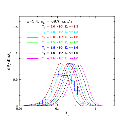
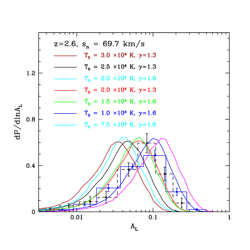
The measurements in our next redshift bin ($\bar{z}=3.4$) suggest the presence of even hotter gas in the IGM (Figure 16). At this redshift the best overall match is the model with $T_{0}=2.5\times 10^{4}$ K, $\gamma=1.3$. Even a fairly hot model with $T_{0}\sim 2\times 10^{4}$ K, $\gamma=1.3$ produces too few low wavelet amplitude regions, and too many high amplitude ones. Models with lower temperatures are clearly quite discrepant. At this redshift, the measured PDF is a bit wider than the simulated ones. This might owe to temperature inhomogeneities, or it may indicate some metal line contamination since, as with the $\bar{z}=4.2$ data, we have not identified and excised metal lines in this redshift bin. In either of these cases, the measurements may allow for some even hotter gas at $T_{0}\sim 3\times 10^{4}$ K.

Figure 17.— Comparison between the measured wavelet PDF in the $\bar{z}=3.0$ bin with $s_{m}=69.7$ km/s and simulated models. Similar to Figure 15–Figure 16, but at $\bar{z}=3.0$. The blue histogram shows the PDF estimated from all spectral regions, while the black dashed histogram removes regions with metal line contamination. The histogram with metal contaminated regions removed comes from the subset of the data in this redshift bin for which we have identified metals.

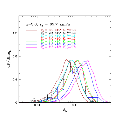
The measurements at $\bar{z}=3.0$ indicate similarly hot gas (Figure 17). By this redshift, the average absorption in the forest is increased and the wavelet PDF is most sensitive to gas a little more dense than the cosmic mean, at roughly $1+\delta=\Delta\sim 2$ for our method. This means that models that have a lower temperature at mean density ($T_{0}$), yet a steeper temperature-density relation ($\gamma$) give similar wavelet PDFs to models with higher $T_{0}$ and flatter $\gamma$ at this redshift. This explains why the model curves with $T_{0}=2.5\times 10^{4}$ K, $\gamma=1.3$ and $T_{0}=2\times 10^{4}$ K, $\gamma=1.6$ are nearly identical to each other, as are the models with $T_{0}=2\times 10^{4}$ K, $\gamma=1.3$, and $T_{0}=1.5\times 10^{4}$ K, $\gamma=1.6$. At this redshift, the metal line correction appears fairly important: it shifts the peak of the PDF to lower amplitude and narrows the histogram somewhat (as seen by comparing the black dashed histogram and the blue solid histogram in the figure). The error bars are significantly larger for the metal-cleaned measurement than for the full measurement. This is mostly because we only have metal line identifications for some of the spectra in this bin and the metal-cleaned measurement hence comes from a smaller number of spectra, and also because we use a smaller portion of each spectrum after metal cleaning. The mean wavelet amplitude changes by less than the $1-\sigma$ error bar as we vary $f_{m}$ between $f_{m}=0.8$ and $f_{m}=1$, and so $f_{m}=0.95$ is a conservative choice, and we hence stick to this choice throughout. After accounting for metal contamination, the model curves with $T_{0}=2\times 10^{4}$ K, $\gamma=1.3$, and $T_{0}=1.5\times 10^{4}$ K, $\gamma=1.6$ are somewhat disfavored. Again, the cooler models with $T_{0}=7,500-10,000$ K differ strongly with the measurement, regardless of the metal correction. The hottest model shown with $T_{0}=3.0\times 10^{4}$ K, $\gamma=1.3$ produces too many low-amplitude, and two few high amplitude regions. The models with $T_{0}=2.5\times 10^{4}$ K, $\gamma=1.3$ and $T_{0}=2.0\times 10^{4}$ K, $\gamma=1.6$ are strongly degenerate and each roughly match the measured PDF.

Figure 18.— Comparison between the measured wavelet PDF in the $\bar{z}=2.6$ bin with $s_{m}=69.7$ km/s and simulated models. Similar to Figure 15–Figure 17, but at $\bar{z}=2.6$.

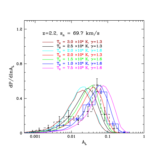
Proceeding to lower redshift, the data at $\bar{z}=2.6$ disfavor some of the hotter IGM models (Figure 18). At this redshift, the models shown with $T_{0}=3.0\times 10^{4}$ K, $\gamma=1.3$; $T_{0}=2.5\times 10^{4}$ K, $\gamma=1.3$; $T_{0}=2.0\times 10^{4}$ K, $\gamma=1.6$ all produce too many low amplitude regions, and too few high amplitude ones. The other models shown with $T_{0}=2.0\times 10^{4}$ K, $\gamma=1.3$; $T_{0}=1.5\times 10^{4}$ K, $\gamma=1.6$, and $T_{0}=1.0\times 10^{4}$ K, $\gamma=1.6$ are closer to the measurements, although none of the models are a great fit. The cooler model with $T_{0}\sim 7,500$ K is again a poor match to the measurement. The preference for somewhat more moderate temperatures at this redshift may result from cooling after HeII reionization completes at higher redshift.

Figure 19.— Comparison between the measured wavelet PDF in the $\bar{z}=2.2$ bin with $s_{m}=69.7$ km/s and simulated models. Similar to Figure 15–Figure 17, but at $\bar{z}=2.2$.

Finally, the measurement in the $\bar{z}=2.2$ bin is shown in Figure 19. The general features are similar to the results at $\bar{z}=2.6$: the hotter models are clearly a poor match to the data, and there is some preference for cooler temperatures, although none of the models are a great match to the data. The models with $(T_{0},\gamma)=(2.0\times 10^{4}K,1.3),(1.5\times 10^{4}K,1.6)$ and $(1.0\times 10^{4}K,\gamma=1.6)$ are the closest matches of the models shown. At this redshift, the mean transmission is high ($\langle F\rangle=0.849$), and the method is sensitive to somewhat overdense gas as a result. The similarity between the models with $T_{0}=3.0\times 10^{4}$ K, $\gamma=1.3$ and $T_{0}=2.0\times 10^{4}$ K, $\gamma=1.6$ suggests that the PDFs are most sensitive to densities around $\Delta=3.9$ at this redshift. We expect scatter in the temperature density relation from shock-heating to be most important at this low redshift, especially since the wavelet PDF is becoming sensitive to the temperature of moderately overdense gas. This may be part of the reason for the poorer overall match between simulations, where the effects of shocks on $T$ are ignored in post-processing, and observations at this redshift. We will investigate this in more detail in the future.

In summary, our measurements appear to support a picture where the IGM is being heated in the middle of the redshift range probed by our data sample, with the temperature likely peaking between $z=3.0-3.8$, before cooling down towards lower redshifts. The favored peak temperature appears to be around $T_{0}\sim 25-30,000$ K, somewhat hotter than found by most previous authors (see §4.10), although consistent with theoretical expectations from photoheating during HeII reionization, especially if the quasar ionizing spectrum is on the hard side of the models considered by McQuinn et al. (2008) (see their Figure 12).

4.3. Uncertainties in the Underlying Cosmology and Mean Transmitted Flux

In the previous section we showed model wavelet PDFs for varying temperature-density relations, but left the underlying cosmology and mean transmitted flux fixed. Here we consider how much the wavelet PDF varies with changes in these quantities. As far as the underlying cosmology is concerned, we restrict our discussion to uncertainties in the amplitude of density fluctuations. Note that there is some ($2-\sigma$ level) tension between the amplitude of density fluctuations determined from the Ly-$\alpha$ forest and WMAP constraints (Seljak et al. 2006).

Figure 20.— Sensitivity of the wavelet PDF to the amplitude of underlying density fluctuations. The model curves show the wavelet PDF for mock spectra generated using simulation snapshots at a range of redshifts for an otherwise identical model. Snapshots at lower redshift approximate models in which the amplitude of underlying density fluctuations is higher than our fiducial value, while the curve generated from the $z=4.5$ model (blue dashed line) approximates a model with a lower amplitude of density fluctuations.

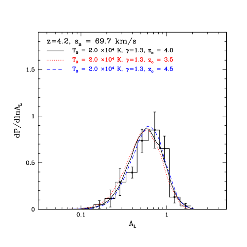
In order to gauge the impact of uncertainties in the amplitude of density fluctuations, we generate mock spectra for a given model using simulation outputs of varying redshift. In particular, we consider a model at $\bar{z}=4.2$ with $\langle F\rangle=0.346$, $T_{0}=2\times 10^{4}$ K, and $\gamma=1.3$, which roughly matches the measured PDF. We generate mock spectra in this model from outputs at $z_{o}=3.5,4.0$, and $4.5$. For the prediction in our fiducial cosmology, we linearly interpolate between wavelet PDFs generated from the $z=4.0$ and $z=4.5$ outputs. Using instead the model PDFs at $z_{o}=3.5$ or $4.0$ (with the mean transmitted flux fixed at $\langle F\rangle=0.346$) – in which structure formation is more advanced – should mimic a model with a higher amplitude of density fluctuations, while using the $z=4.5$ snapshot should correspond to a model with smaller density fluctuations. Our fiducial model has $\sigma_{8}(z=0)=0.82$, roughly in between the preferred values inferred from the forest alone and that from WMAP-3 alone (Seljak et al. 2006). Using the outputs at $z_{o}=3.5,4.0$, and $4.5$ for the $\bar{z}=4.2$ mock spectra should roughly correspond to models with $\sigma_{8}(z=0)=0.95,0.85$ and $0.78$ respectively. The results of these calculations, shown in Figure 20, illustrate that the wavelet PDF is only weakly sensitive to the underlying amplitude of density fluctuations. The mean small-scale power is exponentially sensitive to the temperature, which is uncertain at the factor of $\sim 2$ level, and so it is unsurprising that $\sim 10\%$ level changes in the amplitude of density fluctuations have relatively little impact. The small effect visible in the plot is that the wavelet PDF shifts to smaller amplitudes for the outputs in which structure formation is more advanced. This likely owes to the enhanced peculiar velocities in models with larger density fluctuations, which suppress the small-scale fluctuations in the forest via a finger-of-god effect (e.g. McDonald et al. 2006). The impact of uncertainties in the amplitude of density fluctuations on the wavelet PDF are similarly small at other redshifts, and so we do not discuss this further here.

The amplitude of fluctuations in the forest, and the wavelet PDF, are sensitive to the mean transmitted flux and uncertainties in this quantity impact constraints on the temperature from the PDF measurements. The mean transmitted flux partly determines the ‘bias’ between fluctuations in the transmission and the underlying density fluctuations, with the bias increasing as the mean transmitted flux decreases. This impacts the small-scale transmission power spectrum, and the wavelet PDF, as well as fluctuations on larger scales. When the gas density is sufficiently high, and/or the ionizing background sufficiently low – i.e., when the mean transmitted flux is small – even slight density inhomogeneities produce absorption features, yielding large transmission fluctuations on small-scales.

In the previous section, we adopted the best fit values of the mean transmitted flux from Faucher-Giguère et al. (2008b), but now consider variations around these values. These authors provide estimates of the statistical and systematic errors on their mean transmitted flux measurements. Their $1-\sigma$ errors at our bin centers are: $(z,\langle F\rangle\pm 1-\sigma)=(2.2,0.849\pm 0.017),(2.6,0.778\pm 0.017),(3.0,0.680\pm 0.02),(3.4,0.566\pm 0.022),(4.2,0.346\pm 0.042)$. Their systematic error budget accounts for uncertainties in estimating metal line contamination, and for uncertainties in corrections related to the rarity of true unabsorbed regions at high redshift, among other issues. Nonetheless, there is some tension between the measurements of different groups. We refer the reader to Faucher-Giguère et al. (2008b) for a discussion.

Figure 21.— Impact of uncertainties in the mean transmitted flux at $\bar{z}=3.4$. The black solid line shows the wavelet PDF in a model with the best fit mean transmitted flux from Faucher-Giguère et al. (2008b). The red dotted line shows the same model, except adopting a mean transmitted flux that is $1-\sigma$ less than the best fit value. The blue dashed line shows the same, except for a mean transmitted flux $1-\sigma$ larger than the best fit. The magenta line shows a cooler IGM model, where the mean transmitted flux is $2-\sigma$ higher than the best fit.

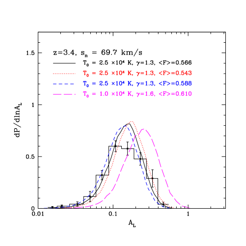
Below $z\lesssim 4$ uncertainties in the mean transmitted flux have a noticeable yet fairly small impact on our constraints. A typical example, in the $\bar{z}=3.4$ redshift bin, is shown in Figure 21. The solid black line in the figure shows a model with $T_{0}=2.5\times 10^{4}$ K, $\gamma=1.3$ that adopts the best fit value for the mean transmission, $\langle F\rangle=0.566$. The blue dashed line is the same model, but with the mean transmitted flux shifted up from the central value by $1-\sigma$. This reduces the amplitude of transmission fluctuations in the model, and shifts the wavelet PDF towards slightly lower amplitudes. Reducing the transmission by $1-\sigma$ has the opposite effect of boosting the typical wavelet amplitudes slightly, as illustrated by the red dotted line in the figure. While the uncertainty in the mean transmitted flux can shift the preferred temperature around slightly, the effect at this redshift is relatively small and has little impact on our main conclusions. For example, a cooler IGM model with $T_{0}=1.0\times 10^{4}$ K and $\gamma=1.6$ still differs greatly from the PDF measurement, even after assuming a mean transmitted flux that is $2-\sigma$ higher than the central value. This is demonstrated by the magenta line in Figure 21.

Figure 22.— Impact of uncertainties in the mean transmitted flux at $\bar{z}=4.2$. Similar to Figure 22, except at $\bar{z}=4.2$.

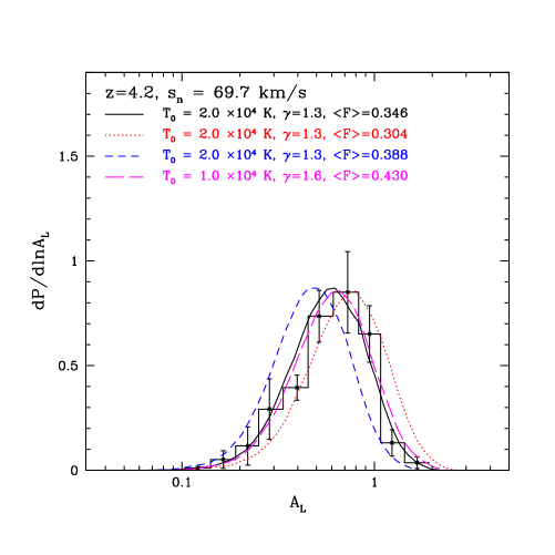
The impact of uncertainties in the mean transmitted flux is more important in our highest redshift bin, at $\bar{z}=4.2$. The impact is larger at this redshift both because data samples are smaller and the fractional error on the mean transmitted flux is larger at this redshift, and because the wavelet amplitudes are more sensitive to the mean transmission once the transmission is sufficiently small. We repeat the exercise of the previous figure at $\bar{z}=4.2$ and present the results in Figure 22. In this case, the model that roughly goes through the PDF measurement with our best fit mean transmitted flux has $T_{0}=2.0\times 10^{4}$ K, and $\gamma=1.3$. After shifting the mean transmitted flux up in this model by $1-\sigma$ it produces too many low wavelet amplitude regions, and too few high amplitude ones, in comparison to the measurement. Indeed, at this redshift, even the cooler IGM model with $T_{0}=1.0\times 10^{4}$ K, $\gamma=1.6$ will pass through the measurement after a $2-\sigma$ upwards shift in the mean transmitted flux. In other words, accounting for uncertainties in the mean transmitted flux, the cool IGM model with $T_{0}=1.0\times 10^{4}$ K, $\gamma=1.6$ can only be excluded at roughly the $2-\sigma$ level.

Furthermore, systematic concerns with direct continuum-fitting are most severe at high redshift, and the agreement between different measurements, while generally good at lower redshifts, is marginal above $z\sim 4$ or so (Faucher-Giguère et al. 2008b). Direct continuum measurements must correct for the fact that there are few genuinely unabsorbed regions at high redshift, which can cause one to systematically underestimate the mean transmitted flux. Part of the disagreement can be traced to the fact that some of the measurements in the literature do not make this important correction. Since Faucher-Giguère et al. (2008b) make a correction using cosmological simulations, we consider their measurement to be more reliable than many of the other previous measurements. However, McDonald et al. (2006) constrain the mean transmitted flux based on a multi-parameter fit to their SDSS power spectrum measurements, which should be immune to this concern. Their best fit to the redshift evolution of the mean transmitted flux gives $\langle F\rangle=0.41$ at $z=4.2$. This disagrees with the Faucher-Giguère et al. (2008b) measurement at this redshift by $1.6-\sigma$. The overall disagreement is in fact more severe than this, because there is a similar level of disagreement in neighboring redshift bins. Dall’Aglio et al. (2008) also perform a direct continuum-fit, correct for the rarity of unabsorbed regions at high redshift with a different methodology, and find a best fit to the redshift evolution of the opacity of $\langle F\rangle=0.40$ at $z=4.2$. Again, this measurement is in tension with the measurement we adopt. Adopting either of these measurements for the best fit mean transmitted flux would favor a cooler IGM temperature.

4.4. Dependence on Large-Scale Smoothing

The measured PDF in the $\bar{z}=3.4$ redshift bin requires hot ($T_{0}\gtrsim 20,000$ K) gas. Interestingly, the PDF in this redshift bin is somewhat broader than the theoretical model curves, which assume a homogeneous temperature-density relation. This may be the result of uncleaned metal line contamination, but a more interesting possibility is that the wide measured PDF indicates temperature inhomogeneities from ongoing HeII reionization. We argued in §2.3 that the precise choice of large scale smoothing, $L$, should be relatively unimportant. Nevertheless, to further explore the exciting possibility that the data indicate temperature inhomogeneities in this redshift bin, we measure the PDF for a few additional choices of $L$ and compare with theoretical models.

Figure 23.— Wavelet PDF at $\bar{z}=3.4$ as a function of large scale smoothing, $L$. The blue histogram in the panels is the wavelet PDF for a large-scale smoothing $L$ of Top–Bottom: $200;1,000;2,000$; and $5,000$ km/s. The color code for the different temperature-density relation models is identical to that in Figure 16.

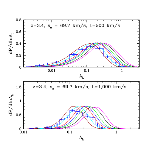
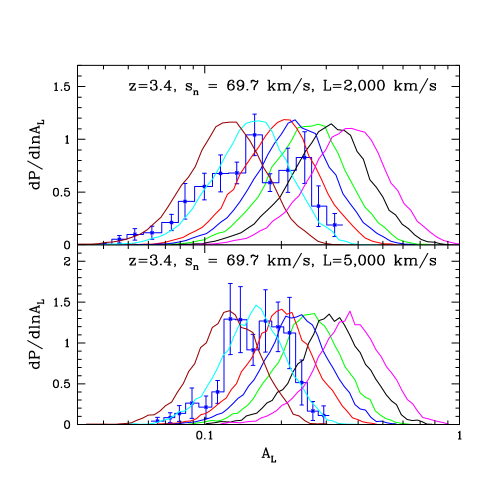
The results of these calculations are shown in Figure 23. In addition to our usual large scale smoothing of $L=1,000$ km/s, we also compare simulated and observational wavelet PDFs for $L=200;2,000;$ and $5,000$ km/s. Here we use $15$ logarithmically spaced $A_{L}$ bins for the PDF measurement, rather than $10$ as in the previous sections, to increase our sensitivity to any bi-modality in the PDF. The mean of the model curves with different smoothing scales is of course fixed, while the width of the PDF increases with decreasing smoothing scale (see §2.3, Figure 6). At all smoothing scales, the simulated model with $T_{0}=25,000$ K and $\gamma=1.3$ is the best overall match to the data. The fit is poorest at $L=2,000$ km/s, but it is not clear precisely how to interpret this since the model is a formally poor fit at each smoothing scale. There does appear to be a slight, yet tantalizing, hint that the PDF is bimodal on large smoothing scales: this trend is most apparent at $L=2,000$ km/s and $L=5,000$ km/s. This may be a first indication of temperature inhomogeneities from ongoing HeII reionization, or it may be the result of uncleaned metal line contamination, as the abundance of metals can vary significantly on large smoothing scales. It will be interesting to revisit this measurement with larger data samples in the future.

4.5. Dependence on Small-Scale Smoothing

We found in the previous sections that our results at $s_{n}=34.9$ km/s are quite susceptible to metal-line contamination and somewhat to shot-noise bias. Because of this, we will not presently use the results at this smoothing scale in constraining the thermal history of the IGM. Nevertheless, as a consistency check we compare here the measured wavelet PDF at this smoothing scale with simulated models.

Figure 24.— Wavelet PDFs for the $s_{n}=34.9$ km/s filter at $\bar{z}=3.0,2.6$ and $\bar{z}=2.2$ (from Top – Bottom). Similar to previous plots at $s_{n}=69.7$ km/s, the black dashed histograms with error bars show the measured wavelet PDFs, corrected for metal line contamination. The blue solid histogram is the same, without masking metal lines. A few example model curves are shown at each redshift, with random noise added to the mock spectra. The models that match the measurements at this smoothing are similar to the ones at the larger smoothing scale.

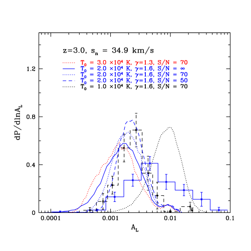
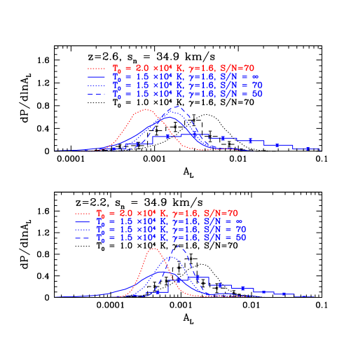
As mentioned previously, to guard against shot-noise bias, we cut spectra with a (red-side) $S/N\leq 50$ and add random noise to the mock spectra. Provided we cut out the low $S/N$ data, the random noise mainly impacts only the low wavelet amplitude tail by decreasing the number of very low amplitude wavelet regions. We add Poisson distributed noise to the mock spectra, assuming that the noise is dominated by Poisson fluctuations in the photon counts from the quasar itself. We have experimented with incorporating Poisson distributed sky noise, and Gaussian random read-noise, and find qualitatively similar results at fixed noise level. We estimate the average wavelet amplitude in the forest contributed by noise (after our $S/N$ cut) as described in Appendix A, and find that it corresponds to $S/N\sim 70$, per $4.4$ km/s pixel at the continuum for the $\bar{z}=3.0$ bin. In Figure 24 we compare some example model PDFs with the measurements, and find results gratifyingly close to those at larger smoothing scale. In particular, the model with $T_{0}=2.0\times 10^{4}$ K, and $\gamma=1.6$ at $\bar{z}=3.0$ that roughly matched the measurement on larger scales, matches the PDF on this smaller scale as well. For contrast, we show a hotter and a colder IGM model which are again a poor match. At $\bar{z}=2.2$ and $\bar{z}=2.6$ the results are similar to the previous ones, suggesting a cooler IGM at these redshifts. Comparing the blue and black dashed histograms, it is clear that the metal contamination correction is quite important at this scale and we do not use these results in what follows.

We have also compared the $s_{n}=34.9$ km/s wavelet PDF in the two highest redshift bins – where we have not identified metal lines – with model PDFs. The measured PDF at $z=3.4$ looks similar to the $T_{0}=2.5\times 10^{4}$ K, $\gamma=1.3$ model that we previously identified as the best general match of our example models at $s_{n}=69.7$ km/s, except with a fairly prominent tail towards high wavelet amplitudes. We expect more significant metal contamination at this smoothing scale (Appendix B), and so this is in line with our expectations. Indeed, the tail towards high wavelet amplitude looks similar to the one in the top panel of Figure 32. Similar conclusions hold at $z=4.2$, except the agreement without excising metals is better, likely owing to the smaller impact of metals at this redshift (Appendix B).

4.6. Approximate Constraints on the Thermal History of the IGM

In this section, we perform a preliminary likelihood analysis, in order to provide a more quantitative constraint on the thermal history of the IGM from the wavelet measurements. We confine our analysis to a three-dimensional parameter space, spanning a range of values for $T_{0},\gamma$, and $\langle F\rangle$. The results of the previous section suggest that CDM models close to a WMAP-5 cosmology should all give similar wavelet PDFs, and so it should be unnecessary to vary the cosmological parameters in this analysis. In order to facilitate this calculation, we adopt here an approximate approach to cover the relevant parameter space. We generate the wavelet PDF for a range of models by expanding around a fiducial model in a first order Taylor series (see Viel & Haehnelt 2006 for a similar approach applied to SDSS flux power spectrum data). In particular let p denote a vector in the three-dimensional parameter space. Then we calculate the wavelet PDF at a point in parameter space assuming that:

$$P(A_{L},{\mathchoice{{\hbox{\BFd p}}}{{\hbox{\BFt p}}}{{\hbox{\BFs p}}}{{\hbox{\BFss p}}}})= P(A_{L},{\mathchoice{{\hbox{\BFd p}}}{{\hbox{\BFt p}}}{{\hbox{\BFs p}}}{{\hbox{\BFss p}}}^{0}})+$$ (11)

$$\sum_{i=1}^{3}\frac{\partial P(A_{L},p_{i})}{\partial p_{i}}\bigg{|}_{{\mathchoice{{\hbox{\BFd p}}}{{\hbox{\BFt p}}}{{\hbox{\BFs p}}}{{\hbox{\BFss p}}}}={\mathchoice{{\hbox{\BFd p}}}{{\hbox{\BFt p}}}{{\hbox{\BFs p}}}{{\hbox{\BFss p}}}^{0}}}(p_{i}-p^{0}_{i}).$$

Although inexact, this approach suffices to determine degeneracy directions, approximate confidence intervals, and the main trends with redshift. We use the results of the previous section to choose the fiducial model to expand around: at each redshift we choose the best match of the example models in the previous section as the fiducial model. Using the Taylor expansion approximation of Equation 11, we then estimate the wavelet PDF for a large range of models, spanning $T_{0}=5,000-35,000$ K, $\gamma=1.0-1.6$, and $\langle F\rangle=F_{c}\pm 3\sigma_{F}$ (subject to a $\langle F\rangle$ prior). Here $F_{c}$ denotes the central value from Faucher-Giguère et al. (2008b), and $\sigma_{F}$ denotes their estimate of the $1-\sigma$ uncertainty on the mean transmitted flux. For each model PDF in the parameter space, we first compute $\chi^{2}$ between the model and the wavelet PDF data, ignoring off-diagonal terms in the co-variance matrix. We then add to this $\chi^{2}$ an additional term to account for the difference between the model mean transmitted flux and the best fit value of Faucher-Giguère et al. (2008b). Finally, we marginalize over $\langle F\rangle$ (subject to the above prior based on the results of Faucher-Giguère et al. (2008b)) to compute two-dimensional likelihood surfaces in the $T_{0}-\gamma$ plane at each redshift, and marginalize over $\gamma$ to obtain reduced, one-dimensional likelihoods for $T_{0}$. We assume Gaussian statistics, so that $1-\sigma$ ($2-\sigma$) two-dimensional likelihood regions correspond to $\Delta\chi^{2}=2.30(6.17)$, while one-dimensional constraints correspond to $\Delta\chi^{2}=1(4)$.

The best fit models at $z=4.2,3.4,3.0,2.6,$ and $2.2$ have $\chi^{2}=9.5,19.8,5.7,8.0,$ and $23.1$ respectively for $7$ degrees of freedom (10 $A_{L}$ bins minus $1$ constraint since the PDF normalizes to unity, minus two free parameters). The fits at $z=4.2$, $3.0$, and $2.6$ are acceptable, while the $\chi^{2}$ values in the $z=3.4$ and $z=2.2$ bins are high (p-values of $6\times 10^{-3}$ and $2\times 10^{-3}$ respectively). The poor $\chi^{2}$ in these redshift bins results because the measured PDFs are broader than the theoretical models in these bins, as discussed previously. We will nevertheless consider how $\chi^{2}$ changes around the best fit models in these redshift bins, although we caution against taking the results too literally.

Figure 25.— Approximate constraints in the $T_{0}-\gamma$ plane. The panels show $1-\sigma$ (red) and $2-\sigma$ (blue) constraints in the $T_{0}-\gamma$ plane at different redshifts, marginalized over the mean transmitted flux.

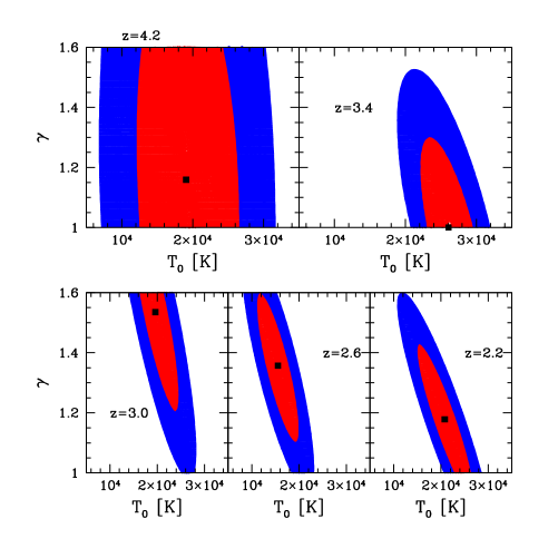
The constraints from these calculations are shown in Figure 25 and Figure 26. They are qualitatively consistent with the example models shown in the previous section. The degeneracy direction of the constraint ellipses results because the $z=4.2$ measurements are sensitive only to the temperature close to the cosmic mean density, while the lower redshift measurements start to constrain only the temperature of more overdense gas. The best fit model at $z=4.2$ has $T_{0}\sim 20,000$ K, but uncertainties in the mean transmitted flux allow cooler models with $T_{0}\sim 10,000$ K at $\sim 2-\sigma$, as discussed previously. The $z=3.4$ measurements indicate the largest temperatures, and require that $T_{0}\gtrsim 20,000$ K at $2-\sigma$ confidence. The lower redshift measurements, particularly that at $z=2.6$, generally favor cooler temperatures although at only moderate statistical significance.

Figure 26.— Approximate constraints on $T_{0}$ as a function of redshift. The red points and error bars show $2-\sigma$ constraints on the temperature at mean density in each redshift bin, after marginalizing over $\langle F\rangle$ and $\gamma$ at each redshift. The dotted, dashed and dot-dashed lines are for comparison. The black dotted line varies as $(1+z)^{2}$, after passing through the highest temperature point at $z=3.4$. The upper blue dashed line shows a model in which HI/HeI reionization completes late, the IGM is reionized to a high temperature, and HeII is not yet reionized. The lower blue dashed line is similar, except in this case HI/HeI reionize early. The black dot-dashed line is for a model in which HI/HeI/HeII are all reionized together at $z=6$ by sources with a quasar like spectrum. This curve is roughly an upper limit to the temperature without late time HeII reionization. A flat $T_{0}\sim 20,000$ K thermal history is consistent within the errors, but an implausibly hard ionizing spectrum is required to achieve such a high temperature from residual photoheating after reionization. This comparison suggests late time HeII reionization, perhaps completing near $z\sim 3.4$.

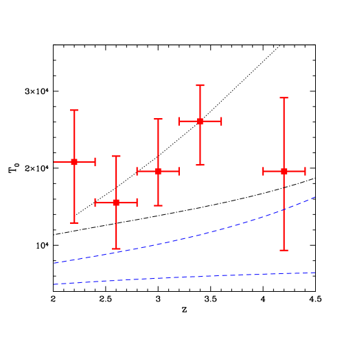
Figure 26 shows ($2-\sigma$) constraints on the temperature at mean density after marginalizing over $\gamma$ and $\langle F\rangle$. We conservatively allow $\gamma$ to vary over $\gamma=1.0-1.6$, even though $\gamma\gtrsim 1.2$ is expected theoretically (McQuinn et al. 2008). If we enforced a prior that $\gamma$ be steeper than $1.2$, then the results at $z\lesssim 3.4$ would disfavor some of the higher $T_{0}$ models. The $T_{0}$ results are consistent with the IGM temperature falling off as $T_{0}\propto(1+z)^{2}$ below $z=3.4$, i.e., below this redshift the temperature evolution appears consistent with simple adiabatic cooling owing to the expansion of the Universe. Theoretically, we expect the temperature fall-off to be similar, but slightly slower, than the adiabatic case just after reionization with the temperature evolution eventually slowing owing to residual photoionization heating (Hui & Gnedin 1997). The statistical errors are however still large, and a flat temperature evolution is also consistent with the $T_{0}$ constraints, although this case is disfavored theoretically (see below). Note also that enforcing a $\gamma\geq 1.2$ prior would disfavor the high $T_{0}$ models that are otherwise allowed at $z=2.2$ and $z=2.6$, strengthening the case for cooling below $z\sim 3.4$.

Moreover, the high temperatures at $z=3.0$ and $z=3.4$ suggest recent HeII photoheating. To illustrate this point, we show several example thermal history models in Figure 26, considering both cases without any HeII photoheating, and ones in which HI/HeI/HeII are all reionized together at high redshift ($z\geq 6$). The upper blue dashed line is a late HI reionization model ($z_{r}=6$), with a high temperature at reionization ($T_{r}=3\times 10^{4}K$), and a hard spectrum near the HI/HeI ionization thresholds (with a specific intensity near threshold of $J_{\nu}\propto\nu^{-\alpha}$ and $\alpha=0$). This case should roughly indicate the highest possible temperature without HeII photoheating over the redshift range probed. Note that this is a rather extreme situation, since even if reionization completes as late as $z=6$, much of the volume will be reionized significantly earlier (e.g. Lidz et al. 2007). The lower blue dashed line is an early reionization model ($z_{r}=12$ and $\alpha=2$) that approximately indicates the lowest plausible temperature without HeII photoheating.

Finally, perhaps the most interesting case is the black dot-dashed line which shows a model in which HI/HeI/HEII are all reionized together at $z=6$. Here we assume that the temperature at reionization is $T_{r}=3\times 10^{4}K$, since atomic hydrogen line cooling should keep the temperature less than this when all three species are ionized simultaneously (Miralda-Escudé & Ress 1994, Abel & Haehnelt 1999, Lidz et al., in prep). The temperature after reionization depends on the ionizing spectrum, which determines the amount of residual photoheating. The curve here adopts a quasar like spectrum, reprocessed by intervening absorption, to give $\alpha_{\rm HI}=1.5$ near the HI ionization threshold and $\alpha_{\rm HeII}=0$ near the HeII ionization threshold (Hui & Haiman 2003). This case is hence similar to the other $z=6$ reionization model, except with the addition of residual HeII photoheating. Each of the examples considered gives too low a temperature in the $z=2.2$, $z=3.0$, and $z=3.4$ redshift bins, particularly at $z=3.4$ and $z=3$. One can further ask how hard the post-reionization ionizing spectrum would need to be to give a thermal asymptote as large as $\sim 20,000$ K. For a power law spectrum we find, using the thermal asymptote formula of Hui & Haiman (2003), that an implausibly hard spectrum with $\alpha\lesssim-0.73$ is required to match the $2-\sigma$ lower limit on the $z=3.4$ temperature. In fact, there is evidence that galaxies rather than quasars produce most of the ionizing background at $z\gtrsim 3$ (e.g. Faucher-Giguère et al. 2008b), and so assuming even a quasar like spectrum likely overestimates residual photoheating for plausible early HeII reionization models. In summary, although the errors allow the possibility of a slow temperature evolution and $T_{0}\sim 20,000$ K, this temperature is higher than expected from residual photoheating long after reionization.

The simplest interpretation is that HeII reionization heats the IGM, with the process completing near $z\sim 3.4$, at which point there is relatively little additional heating and the Universe expands and cools. The redshift extent over which the heat input occurs is, however, not well constrained by our present measurement. Clearly the large error bars on the measurements still leave room for other possibilities. For example, models in which HeII reionization completes a bit later at $z\sim 3$ – or perhaps even as late as $z\sim 2.7$ as favored by a recent analysis of HeII Ly-$\alpha$ forest data by Dixon & Furlanetto 2009 – or earlier at $z\sim 4$ are likely consistent with our present measurements given the large error bars. We will consider this further in future work. Finally, other heating mechanisms may be at work in addition to photoionization heating.

4.7. An Inverted Temperature-Density Relation?

Recently, Bolton et al. (2008), Becker et al. (2007) and Viel et al. (2009) have suggested that measurements of the Ly-$\alpha$ flux PDF favor an inverted temperature density relation ($\gamma<1$), i.e., situations where low density gas elements are hotter than overdense ones. Bolton et al. (2008) and Viel et al. (2009) construct simulated models with inverted temperature-density relations by adding heat into the simulations in a way that depends on the local density, i.e., on the density smoothed on the Jeans scale. This particular case for an inverted temperature-density relation seems unphysical to us since heat input from, e.g. reionization, should be coherent on much larger scales. Nonetheless, we can consider this as a phenomenological example that the flux PDF data favor, and examine the implications of these models for the small-scale wavelet amplitudes. Theoretically, Trac et al. (2008) and Furlanetto & Oh (2009) find that hydrogen reionization does produce a weakly inverted temperature-density relation. This effect is driven by the tendency for large-scale overdensities to reionize hydrogen first, coupled presumably with the small correlation between the overdensity on large scales and that on the Jeans scale. On the other hand, McQuinn et al. (2008) find that HeII reionization leads to a non-inverted equation of state with $\gamma\sim 1.3$ in the midst and at the end of HeII reionization. We refer the reader to this paper for further discussion.

Figure 27.— Wavelet PDF in inverted temperature density relation models compared to measurements. The dashed histogram shows the metal line corrected wavelet PDF at $z=3$ ($L=1,000$ km/s, $s_{n}=69.7$ km/s), and the blue histogram is the same without correcting for metal line contamination. The colored lines show several models with $\gamma=0.5$. One can fit the PDF with an inverted temperature density relation, but this requires an extremely high temperature at mean density.

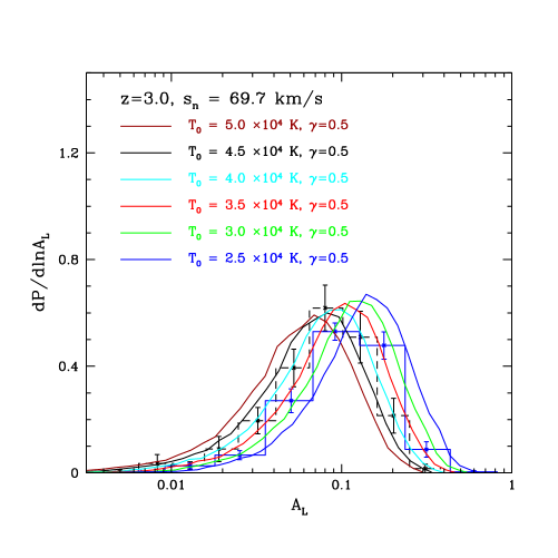
To explore this, we generate mock spectra and measure wavelet amplitudes for several inverted temperature-density relation models and compare with our $z=3$ measurements. As before, we are considering the impact of the temperature in a post-processing step, and so we are not accounting for differences between the gas pressure smoothing in the inverted models and that in the simulation. Likewise, we incorporate thermal broadening assuming a perfect temperature density relation, and so the impact of scatter in the temperature density relation is ignored in this part of the calculation. We consider inverted temperature density relations with a power law index of $\gamma=0.5$, close to the value suggested by Bolton et al. (2008) and Viel et al. (2009) from their flux PDF measurements near $z=3$. The results of these calculations are shown in Figure 27. These cases also roughly match the observed PDF, but require a very high temperature at mean density of $T_{0}\sim 40-45,000$ K. The reason for this is that the wavelet PDF measurements are sensitive mostly to the temperature around a density of $\Delta\sim 2$ at this redshift. In the previous section we found that models with, for example, $T_{0}\sim 25,000$ K and $\gamma=1.3$ roughly match the data. A model with an inverted temperature density relation ($\gamma=0.5$) produces the same temperature at a density of $\Delta\sim 2$ only for a much higher temperature (at mean density) of $T_{0}\sim 45,000$ K. The figure suggests that the expected degeneracy between $T_{0}$ and $\gamma$ indeed extends to even these inverted temperature-density relations. Hence one can fit the measurements with a very high $T_{0}$, small $\gamma$ model, although the inverted cases produce slightly wider PDFs. While these can fit the data, the high required temperatures seem unlikely to us, and we disfavor inverted models for this reason.

Bolton et al. (2008) and Viel et al. (2009) found that inverted models with substantially smaller temperature at mean density match their flux PDF measurements. On the other hand, Viel et al. (2009) did a joint fit to the flux PDF and the SDSS flux power spectrum from McDonald et al. (2006). Recall that the SDSS measurements are sensitive only to the large scale flux power spectrum ($k\lesssim 0.02$ s/km), and thus depend on IGM parameters differently than the small-scale wavelet measurements explored here. Their joint fit requires high $T_{0}$ for cases with inverted temperature-density relations, similar to our conclusions from a different type of measurement. There thus appears to be some tension with the flux PDF measurement, which may reflect systematic errors in one or more of the measurements and/or the modeling. We intend to consider this further in future work.

4.8. Inhomogeneities in the Temperature-Density Relation

Let us further consider the implications of our measurements for the presence or absence of temperature inhomogeneities in the IGM. In most redshift bins, the measured PDF has comparable width to the simulated PDFs, which assume a perfect temperature-density relation. The possible exceptions are the $\bar{z}=3.4$ bin (where metal contamination is a possible culprit) and the $\bar{z}=2.2$ bin (where scatter from shocks may be most important). One might wonder if the widths of the wavelet PDFs are too small to be compatible with ongoing or recent HeII reionization, which is presumably a fairly inhomogeneous process. A related question regards the precise meaning of our temperature constraints in the presence of inhomogeneities: which temperature do we measure exactly – the mean temperature, the minimum temperature, etc.? We intend to address these issues in detail in future work, but we outline a few pertinent points here. In this discussion, we draw on the results of McQuinn et al. (2008).

The first point is that temperature inhomogeneities during HeII reionization, while likely important, are smaller than one might naively guess. McQuinn et al. (2008) emphasized the importance of hard photons, with long mean free paths, for HeII photoheating: much of the heating during HeII reionization by bright quasars occurs far from sources, rather than in well-defined ‘bubbles’ around ionizing sources. This is quite different than during HI/HeI reionization by softer stellar sources, where the ionizing photons have short mean free paths and heating does occur within well-defined bubbles. Since the hard photons have long mean free paths, and a ‘background’ radiation field from multiple sources needs to be built up before these photons appreciably ionize and heat the IGM, the heating is much more homogeneous than might otherwise be expected. The softer photons, typically absorbed in bubbles around the quasar sources, only heat the IGM by $\delta T\lesssim 7,000$ K. Consider the temperature PDFs in Figure 11 of McQuinn et al. (2008). This figure illustrates that by the time any gas is heated significantly, there are very few completely cold regions left over in the IGM: the temperature field is more homogeneous than might be expected.

Simplified models with discrete $\sim 30,000K$ bubbles around quasar sources and a cooler IGM outside (e.g. Lai et al. 2006) are hence not realistic, and overestimate the temperature inhomogeneities. In the McQuinn et al. (2008) simulations, the temperature inhomogeneities peak at a level of $\sigma_{T}/\langle T\rangle\sim 0.2$, which is reached in the early phases of HeII reionization. For contrast, a toy two-phase hot/cold IGM with hot bubbles that are $3$ times as hot as a cooler background IGM, gives a more substantial peak fluctuation level of $\sigma_{T}/\langle T\rangle=0.58$, reached when the hot bubbles fill $25\%$ of the IGM. In the midst of HeII reionization, the McQuinn et al. (2008) simulations predict roughly $10\%$ level temperature fluctuations on large scales from inhomogeneous HeII heating. This level of scatter may be hard to discern with our existing measurement.

Figure 28.— Illustration of the challenge of detecting temperature inhomogeneities. The blue histogram with error bars is the wavelet PDF at $\bar{z}=4.2$ and $s_{n}=69.7$ km/s. The curves show theoretical models: the red line is a hot model, the black line is a cold model, while the blue curve shows a fifty-fifty mix between the hot and cold models. This extreme model can be ruled out as it is too broad, and produces too may high amplitude regions compared to the data, but one can see that detecting smaller levels of inhomogeneity is challenging.

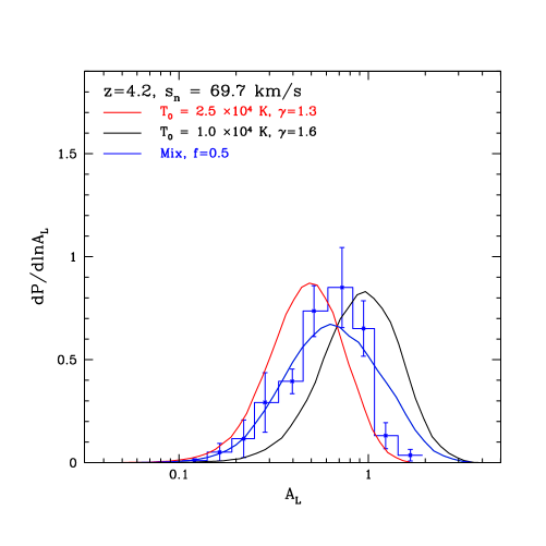
To illustrate this, we compare the $\bar{z}=4.2$, $s_{n}=69.7$ km/s measurement to a simplified and extreme two phase model. This redshift bin probes extended stretches of spectrum along just two lines of sight. Imagine a model where one line of sight passes entirely through cold regions of the IGM with $T_{0}=10^{4}$ K, $\gamma=1.6$, while the other line of sight passes entirely through hot regions with $T_{0}=2.5\times 10^{4}$ K, $\gamma=1.3$. This is a contrived example since each sightline probes hundreds of co-moving Mpc, and so each sightline should in reality probe a mix of temperatures, but this simple case nonetheless illustrates the challenge of detecting temperature inhomogeneities. For simplicity, in this toy model we imagine that each line of sight probes an equal stretch through the IGM so that the wavelet PDF is a fifty-fifty mix of the hot and cold models. In this toy scenario the mean IGM temperature is $\langle T\rangle=17,500$ K and the fluctuation level is $\sigma_{T}/\langle T\rangle\sim 0.43$, i.e., substantially larger than we expect. The wavelet PDF in this toy model is shown in Figure 28. This simple model clearly produces too broad a PDF, but it is also apparent that smaller, likely more realistic, levels of inhomogeneity will be hard to distinguish with the existing data. For example, an inhomogeneous model with fewer cold regions than in the toy two-phase model would agree with the measurement. Indeed, the data may even favor slightly inhomogeneous models, but we leave exploring this to future work. The $z=4.2$ and $z=3.4$ data, which may be in the midst of HeII reionization, and which are sensitive to the temperature near the cosmic mean density, are the best redshift bins for further exploration. Provided the inhomogeneities are relatively small, as suggested by the measurements in most redshift bins, ambiguities in which temperature we constrain precisely are unimportant, and our temperature estimates should be accurate.

Another possible issue, related to the discussion in §2.3, is that the one-dimensional nature of the Ly-$\alpha$ forest may obscure detecting temperature inhomogeneities from HeII reionization. Consider the three-dimensional power spectrum of temperature fluctuations in Figure 10 of McQuinn et al. (2008). There is a large scale peak in the three-dimensional power spectrum, owing to inhomogeneous heating, and a prominent small-scale ramp-up that results from the temperature-density relation and small-scale density inhomogeneities. The large scale peak in the power spectrum is essentially the signal we are after, while the small scale ramp-up is noise as far as extracting inhomogeneities is concerned. However, the one-dimensional temperature power spectrum may be more relevant than the three-dimensional one for absorption spectra. In the one-dimensional temperature power spectrum, high-$k$ transverse modes, which are dominated by the small-scale ramp-up, will be aliased to large scales, swamping the temperature inhomogeneities. This argument is imperfect though, since the one-dimensional temperature power spectrum is not exactly the relevant quantity either: absorption spectra are insensitive to the temperature of large overdensities, which regardless produce saturated absorption. It will be interesting to consider this further in the future, and to consider the potential gains from cross-correlating the wavelet amplitudes of pairs of absorption spectra.

A final issue, particularly relevant in the highest redshift bin, is that the temperature inhomogeneities may depend on the timing and nature of hydrogen reionization. The temperature contrast between regions with doubly ionized helium and those in which only HI/HeI are ionized depends on when hydrogen (and HeI) reionized. Specifically, the temperature contrast between HII/HeII and HII/HeIII regions will be reduced if hydrogen is reionized late to a high temperature, and increased if hydrogen reionizes early to a smaller temperature. Moreover, heating from hydrogen reionization will itself be inhomogeneous (e.g. Cen et al. 2009). Extending the measurements in this paper to higher redshift can help disentangle the impact of hydrogen and helium photoheating. Further modeling will also be helpful.

4.9. The Impact of Jeans Smoothing

As mentioned previously, a shortcoming of our modeling throughout is that we have run only a single simulated thermal history in describing the gas density distribution in the IGM: we vary the thermal state of the gas only as we construct mock absorption spectra and incorporate thermal broadening. Similar approximations are common in the Ly-$\alpha$ forest literature. The gas density distribution is sensitive to the full thermal history of the IGM (Gnedin & Hui 1998) and so properly accounting for a range of thermal histories requires running many simulations. This certainly deserves further exploration, but we do not expect a big impact on our present results. Thermal broadening directly smooths the optical depth field and results in a roughly exponential decrease in small-scale flux power (Zaldarriaga et al. 2001), while Jeans smoothing acts on the three-dimensional gas distribution and has a less direct impact. Properly accounting for the impact of HeII photoheating in the simulation run should smooth out the gas distribution a bit, and reduce the wavelet amplitudes in these models slightly. This might reduce our favored temperatures during HeII reionization, but we expect this effect to be small compared to other uncertainties. Observational studies of the absorption spectra of close quasar pairs may help disentangle the effects of thermal broadening and Jeans smoothing.

4.10. Comparison with Previous Measurements

Figure 29.— Comparison with previous measurements from the literature. The black points with error bars show the redshift evolution of the temperature at mean density favored by our present analysis. The other points show various measurements from the literature.

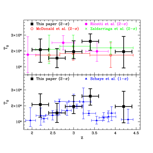
A detailed comparison with previous measurements is difficult since our methodology differs from that of most previous work. Instead, we will simply compare the bottom line, and make a few remarks about the differences. Figure 29 shows our constraints on $T_{0}(z)$, compared to the results of Schaye et al. (2000), Ricotti et al. (2000), McDonald et al. (2001), & Zaldarriaga et al. (2001). It is encouraging that some of the main trends are similar across all of the measurements: for example, all of the measurements favor a fairly hot IGM near $z\sim 3$. In this sense, our work reinforces the previous results. There are differences in the details, however: the peak temperatures in Ricotti et al. (2000), and Schaye et al. (2000) are reached at lower redshift than in our analysis. The McDonald et al. (2001) and Zaldarriaga et al. (2001) results are, on the other hand, flat as a function of redshift, although they adopt wide redshift bins and may average over any temperature increase. Our measurements are also fairly consistent with a flat temperature evolution given the large error bars on our measurements. Our results mostly favor higher temperatures than the previous measurements, particularly the high redshift points of Schaye et al. (2000).

One possible reason for some of the differences is related to improvements in simulations of the forest over the past decade or so. In Appendix A, we found that our method – and we suspect related methods – require fairly large simulation volumes and high mass and spatial resolution, particularly at high redshift (see also e.g. Bolton & Becker 2009). The requisite particle number, while achievable today, was of course prohibitive for past studies. Indeed, this was one of our motivations for revisiting the temperature measurements. While some of the previous studies varied simulation resolution and boxsize, they often considered only a single additional run, which may have been inadequate to fully assess convergence. Finite resolution, in particular, can bias temperature estimates low.

It is instructive to compare our fiducial simulation with a boxsize of $L_{b}=25$ Mpc/$h$ and $N_{p}=2\times 1024^{3}$ particles to the main runs of previous work. Schaye et al. (2000) used a $(L_{b},N_{p})=(2.5$ Mpc/$h$, $2\times 64^{3}$) SPH simulation, Ricotti et al. (2000)’s main runs were ($2.56$ Mpc/$h$, $2\times 256^{3}$) HPM calculations, McDonald et al. (2001) used an Eulerian hydrodynamic simulation with $L_{b}=10$ Mpc/$h$ and $288^{3}$ cells, and Zaldarriaga et al. (2001) used a dark matter only simulation with $L_{b}=16$ Mpc/$h$ and $128^{3}$ dark matter particles. Given the differences between methods, we will not try to estimate the impact of systematic errors from finite boxsize and resolution on previous results. However, it is clear that increases in computing power allow us to do a much better job with respect to boxsize and resolution than previous work. Finally, improved estimates of the mean transmitted flux (Faucher-Giguère et al. 2008b), and improved masking of metal lines, may also contribute to some of the differences between our results and previous work.

5. Cross-correlating with the HeII Ly-$\alpha$ forest

An interesting possibility is to cross-correlate wavelet amplitude measurements from HI Ly-$\alpha$ forest spectra with measurements in the corresponding regions of HeII Ly-$\alpha$ forest spectra. It is timely to consider this, as larger samples of HeII Ly-$\alpha$ forest spectra will soon be available (Syphers et al. 2009), especially given the recent installation of the Cosmic Origins Spectrograph on the Hubble Space Telescope.

A fundamental difficulty with HeII Ly-$\alpha$ forest observations is that the HeII Ly-$\alpha$ cross section is relatively large, and so even a mostly ionized (mostly HeIII) medium may give rise to complete absorption. McQuinn (2009) recently emphasized, however, that this problem is not as acute as it is for the $z\sim 6$ HI Ly-$\alpha$ forest. First, the $z\sim 3$ HeII Ly-$\alpha$ optical depth is significantly smaller than the $z\sim 6$ HI Ly-$\alpha$ optical depth owing to the lower cosmic helium abundance, the smaller absorption cross section, and the lower mean gas density at $z\sim 3$. Moreover, one can locate low density gas elements using high transmission regions from HI Ly-$\alpha$ forest observations of the same quasar: if even these low density regions manage to give complete absorption, these elements and surrounding gas in the absorption trough must be significantly neutral (see McQuinn 2009 for details). As a quantitative measure, it is helpful to note that a gas element at the $z=3$ cosmic mean density with a HeII fraction of only $X_{\rm HeII}=10^{-3}$ produces a significant HeII optical depth of $\tau_{\rm HeII}=3.6$ (e.g. Furlanetto 2008). A gas element at one tenth of the cosmic mean density will give the same optical depth when it is one percent neutral.

While constraining on their own, HeII Ly-$\alpha$ observations may be fruitfully combined with our methodology to extract still more information. Specifically, we propose to measure wavelet amplitudes from the HI Ly-$\alpha$ forest for quasar spectra with existing HeII Ly-$\alpha$ observations, contrasting the wavelet amplitudes in HeII absorption trough regions with those in HeII transmission regions. If the HeII troughs correspond to purely neutral HeII regions, untouched by high energy quasar photons, we expect them to be cold, provided that HeI and HI in the region were ionized long ago, as one expects for absorbing gas at say $z\sim 3-4$. The temperature-density relation in the neutral HeII regions should be at $T_{0}\lesssim 10,000$ K, and $\gamma\sim 1.6$, depending on the nature of the HI ionizing sources, and on when HI reionization occurs (Hui & Haiman 2003). On the other hand, if the regions instead contain mostly ionized HeII (yet are nevertheless opaque in HeII Ly-$\alpha$ owing to the large absorption cross section), they will be at similar temperature to the transmission regions. In this case all of the gas will be hot, unless HeII reionization completed at much higher redshift. A final, somewhat subtle, possibility relates to the fact that towards the end of HeII reionization there will likely be very hot gas elements with neutral fractions as large as $X_{\rm HeII}\sim 0.1$ that are (partly) ionized by a heavily filtered ionizing spectrum from distant quasars (McQuinn et al. 2008). Such regions will give rise to troughs, will generally be hotter than more ionized regions, and occur before HeII reionization completes. Hence, at the end of HeII reionization, we may expect the HeII troughs to be hotter than transmission regions. Only troughs of purely neutral HeII gas, untouched by quasar photons, should be cold. Discovering any cold regions in the HI Ly-$\alpha$ forest that correspond to HeII troughs would also make the presence of cold regions and their connection to HeII reionization more plausible.

Figure 30.— HeII Ly-$\alpha$ troughs and the HI Ly-$\alpha$ wavelet amplitudes. Top panel: The fractional HI Ly-$\alpha$ transmission for the spectrum HE2347-4342. The dashed lines, demarcated by arrows, indicate redshift ranges over which Smette et al.’s (2002) measurements are consistent with complete absorption in the HeII Ly-$\alpha$ forest. Bottom panel: The wavelet amplitudes (with $s_{n}=34.9$ km/s, $L=1,000$ km/s) for the same stretch of spectrum (blue line). The black and red lines are simulated wavelet amplitudes suggesting that even the trough portions of the spectrum are hot and ionized.

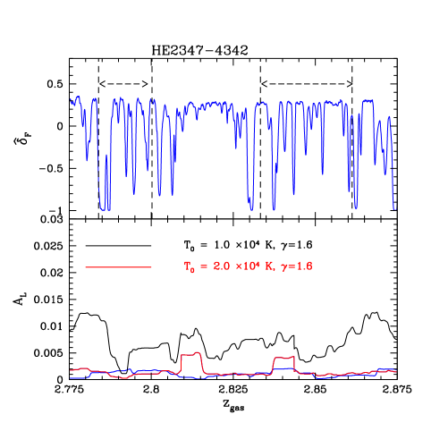
A detailed study of this type will certainly await future HeII Ly-$\alpha$ observations, but we can nevertheless illustrate the main idea with the single spectrum from our sample, HE 2347-4342, for which there is an existing HeII Ly-$\alpha$ forest spectrum (e.g. Smette et al. 2002). These authors identify two spectral regions that are consistent with complete HeII absorption troughs to within the signal to noise of their measurement. Specifically, an observed spectral region between $\lambda_{\rm obs}=1165.00-1173.50\AA$ (an absorption redshift of $\bar{z}_{\rm gas}=2.849$) is estimated to have a mean HeII Ly-$\alpha$ transmission of $\langle F\rangle=-0.001\pm 0.007$, and a region between $\lambda_{\rm obs}=1150.00-1154.95$ ($\bar{z}_{\rm gas}=2.7938$) has $\langle F\rangle=0.024\pm 0.030$ (Smette et al. 2002).

We plot the transmission, $\hat{\delta}_{F}$, for the corresponding portion of the VLT HI Ly-$\alpha$ spectrum in Figure 30 (top panel). In the bottom panel of the figure, we show the wavelet amplitudes (for $s_{n}=34.9$ km/s, $L=1,000$ km/s) of the corresponding stretch of spectrum, and compare it to the amplitude along a typical sightline drawn from a hot $T_{0}=20,000$ K, $\gamma=1.6$ model and a cold $T_{0}=10,000$ K, $\gamma=1.6$ model. The cold model produces larger wavelet amplitudes than the data, and the hot model matches more closely, (although even it has two regions of higher wavelet amplitude than found in the observed spectrum). Hence, our measurement suggests that the high opacity regions are already quite hot. This is unsurprising based on the findings of the previous section that the IGM is mostly quite hot at $z\sim 3$. These special HeII trough regions do not appear cooler than typical regions, and this argues against the gas in these regions being purely neutral. In addition, the trough regions are not obviously hotter than the transmission regions.

We tentatively suggest that the trough regions are hot and ionized. For now, our argument is based only on a small portion of a single spectrum, and so we caution against drawing strong conclusions from it. We regard it as suggestive, and eagerly await further HeII Ly-$\alpha$ spectra to perform a more complete study, hopefully out to higher redshift. Note that there will likely be significant HeII transmission before HeII reionization completes (Furlanetto 2008, McQuinn et al. 2008), and so we should be able to contrast the temperature in trough and transmission regions even in the midst of HeII reionization and fully exploit this method.

6. Conclusions

In this paper, we used a method similar to that of Theuns & Zaroubi (2000) and Zaldarriaga (2002) to quantify the amount of small-scale structure in the Ly-$\alpha$ forest. In particular, we convolved Ly-$\alpha$ forest spectra with suitably chosen Morlet wavelet filters, and recorded the PDF of the smoothed wavelet amplitudes. Using cosmological simulations, we showed that this measure of small-scale structure in the forest can be used to extract information about the temperature of the IGM and its inhomogeneities. We then applied this methodology to $40$ VLT spectra, spanning absorption redshifts between $z=2.2$ and $z=4.2$ and presented tables of the resulting smoothed wavelet PDFs. The tables (Tables 1–5) of smoothed wavelet PDFs are the main result of this paper.

In order to examine the main implications of our measurements for the thermal history of the IGM, we made an initial comparison with high resolution cosmological simulations. This comparison suggests that the temperature of the IGM, close to the cosmic mean density, peaks in the redshift range studied near $z=3.4$, at which point it is hotter than $T_{0}\gtrsim 20,000$ K at $2-\sigma$ confidence. At lower redshift, the data appear roughly consistent with a simple adiabatic fall-off ($T_{0}\propto(1+z)^{2}$) from the peak temperature at $z=3.4$. The high temperature measurements require significant amounts of late time heating, and are inconsistent with models in which HeII reionization completes much before $z\sim 3.4$. At the highest redshift considered, the temperature in our best fit model is rather high, $T_{0}\sim 15-20,000$ K but cooler $T_{0}\sim 10,000$ K models are still allowed at $2-\sigma$ confidence at this redshift, owing mostly to uncertainties in the mean transmitted flux. We believe that the most likely explanation for our results is that HeII reionization completes sometime around $z\sim 3.4$, although the statistical errors are still large and other heating mechanisms may conceivably be at work. In general, our analysis favors higher temperatures and higher redshift HeII reionization than most previous analyses in the literature (see §4.10).

This work can be extended and improved upon in several ways, some theoretical and some observational. First, we intend to compare our measurements to more detailed theoretical models which follow photoheating and radiative transfer during HeII reionization. Next, the wavelet PDF measurements can be combined with measurements of the large scale flux power spectrum from the SDSS (McDonald et al. 2006). This should tighten our constraints, and hopefully break some of the degeneracies present with the mean transmitted flux at high redshift. It would also be interesting to apply our method to a larger data set, beating down the statistical error bars, and filling in the redshift gap in our present data set around $z=3.8$. Identifying metal line absorbers in additional spectra would help further control metal line contamination, an important systematic for small-scale measurements. Particularly interesting would be to apply our methodology at higher redshifts. This would help disentangle the effects of hydrogen and helium photoheating, and perhaps provide interesting constraints on hydrogen reionization (Theuns et al. 2002a, Hui & Haiman 2003). A similar analysis applied to the Ly-$\beta$ region of a quasar spectrum would be sensitive to the temperature of more overdense regions, and help constrain $\gamma(z)$ (Dijkstra et al. 2004). Finally, it would be interesting to consider the implications our our measurements for cosmological parameter constraints from the Ly-$\alpha$ forest, for which the temperature of the IGM is an important nuisance parameter. Although challenging to extract, the small-scale structure in the Ly-$\alpha$ forest contains a wealth of information regarding the thermal and reionization histories of the Universe!

Appendix A: Noise Bias

Here we estimate the shot-noise bias introduced by random noise in the observed quasar spectra. In order to do this, we exploit two features of the underlying signal and noise fields: 1) the smallest measurable scales should be dominated by noise for spectra in which the noise correction is significant, and 2) for white-noise Gaussian random fields, one can filter the field on a very small-scale, labeled here as $s_{m}$, and use this to determine how noise contaminates the moments on larger smoothing scales, $s_{n}$. We confine our discussion here to estimates of the bias in the mean, the variance, and the wavelet amplitude power spectrum, although we ultimately measure the full wavelet PDF.

Let us write the total filtered signal in a quasar spectrum, $a_{n}^{\rm tot}$, as

$$a_{n}^{\rm tot}(x)=a_{n}^{\rm sig}(x)+a_{n}^{\rm noise}(x),$$ (12)

where $a_{n}^{\rm sig}(x)$ denotes the underlying cosmic signal and $a_{n}^{\rm noise}(x)$ is the filtered noise field. If the signal and noise fields are independent, it follows that

$$\langle\hat{A}(x)\rangle=\langle|a_{n}^{\rm tot}(x)|^{2}\rangle=\langle|a_{n}^{\rm sig}(x)|^{2}\rangle+\langle|a_{n}^{\rm noise}(x)|^{2}\rangle.$$ (13)

In other words, provided the signal and noise are uncorrelated, the mean wavelet amplitude we measure, $\hat{A}(x)$, is simply the sum of that from the underlying signal, $A(x)$, and a noise contribution.

We then require $\langle|a_{n}^{\rm noise}(x)|^{2}\rangle$ to estimate the noise bias for the mean wavelet amplitudes. One approach would be to use the pixel noise array estimates produced while performing the spectroscopic data reduction. Here we instead estimate the noise directly from the reduced data, using the total wavelet amplitude (Equation 13) filtered on a smaller scale $s_{m}$. Recall that we normalize the wavelet filters to each have unit power (see Equation 3). This means that the average wavelet amplitude for a white-noise field filtered on scale $s_{m}$ is the same as when the field is instead filtered on scale $s_{n}$: $\langle|a_{m}^{\rm noise}(x)|^{2}\rangle=\langle|a_{n}^{\rm noise}(x)|^{2}\rangle$. Provided we can find a scale $s_{m}$ at which the noise dominates over the signal, that the noise is white-noise, Gaussian random, and that the noise is uncorrelated with the signal, we can construct an un-biased estimator of the signal’s mean wavelet amplitude. We simply subtract the average of the small-scale filtered wavelet amplitudes from that on larger scales. Our estimate of the noise bias comes from filtering the data on a scale $s_{m}=17.4$ km/s, and assuming $\langle|a_{m}^{\rm tot}(x)|^{2}\rangle\sim\langle|a_{m}^{\rm noise}(x)|^{2}\rangle$ on this scale, after metal excision. In a spectrum with low noise, the signal may still dominate over the noise even on this smoothing scale, and in this case we overestimate the noise bias. However, since the signal drops off strongly with wavenumber, we conclude in this case that the noise bias is unimportant.

We would also like to estimate the noise bias in the wavelet amplitude power spectrum, and the bias in the variance of the wavelet amplitudes, smoothed on length scale $L$. To begin with, we neglect any variations in the noise power spectrum, $P_{N}$, from sightline to sightline and assume that it is independent of scale. Using the notation $\hat{A}(x)=|a_{n}^{\rm sig}(x)+a_{n}^{\rm noise}(x)|^{2}$, let us consider the (configuration space) two-point function of $\hat{A}(x)$:

$$\langle\hat{A}(x_{1})\hat{A}(x_{2})\rangle-\langle\hat{A}(x_{1})\rangle\langle\hat{A}(x_{2})\rangle=\xi_{A}^{\rm sig}(|x_{1}-x_{2}|)+\xi_{A}^{\rm noise}(|x_{1}-x_{2}|)$$

$$+\langle a_{n}^{\star\rm sig}(x_{1})a_{n}^{\rm sig}(x_{2})\rangle\langle a_{n}^{\rm noise}(x_{1})a_{n}^{\star\rm noise}(x_{2})\rangle+\langle a_{n}^{\rm sig}(x_{1})a_{n}^{\star\rm sig}(x_{2})\rangle\langle a_{n}^{\star\rm noise}(x_{1})a_{n}^{\rm noise}(x_{2})\rangle$$

$$+\langle a_{n}^{\star\rm sig}(x_{1})a_{n}^{\star\rm sig}(x_{2})\rangle\langle a_{n}^{\rm noise}(x_{1})a_{n}^{\rm noise}(x_{2})\rangle+\langle a_{n}^{\rm sig}(x_{1})a_{n}^{\rm sig}(x_{2})\rangle\langle a_{n}^{\star\rm noise}(x_{1})a_{n}^{\star\rm noise}(x_{2})\rangle.$$ (14)

Here $\xi_{A}^{\rm sig}(|x_{1}-x_{2}|)$ denotes the two-point function of the underlying signal (i.e., Equation 8, although in the above expression we have not yet normalized by $\langle A\rangle$ in the denominator), and $\xi_{A}^{\rm noise}(|x_{1}-x_{2}|)$ is a pure noise term, while the other terms are cross-terms.

The power spectrum of $\hat{A}(x)$ is the Fourier transform of Equation 14. Using the convolution theorem and Equation 3, the pure noise part of the power (i.e., the Fourier transform of $\xi_{A}^{\rm noise}(|x_{1}-x_{2}|)$) can be written as:

$$P_{A}^{\rm noise}(k)=B^{4}P_{N}^{2}\int\frac{dk^{\prime}}{2\pi}\rm{exp}\left[-(k-k^{\prime})^{2}s^{2}+k_{0}^{2}s^{2}\right]\rm{exp}\left[-(k^{\prime}-k_{0})^{2}s^{2}\right].$$ (15)

Here $B=\pi^{-1/4}(2\pi s_{n}/\Delta u)^{1/2}$ is a normalization factor (Equation 3), and we abbreviate $s_{n}$ as $s$. The noise contribution to the wavelet amplitude (squared) power spectrum is proportional to $P_{N}^{2}$ because $A$ is a quadratic function of $\delta_{F}$ (Equations 4–5).

Next we consider the cross terms. The terms on the third line of Equation 14 can be shown to be very small. The important cross terms can be derived by again applying the convolution theorem, and using the Fourier transform of the Morlet Wavelet filter and its complex conjugate. The result is:

$$P_{A}^{\rm cross}(k)= F.T.[\langle a_{n}^{\star\rm sig}(x_{1})a_{n}^{\rm sig}(x_{2})\rangle\langle a_{n}^{\rm noise}(x_{1})a_{n}^{\star\rm noise}(x_{2})\rangle+\langle a_{n}^{\rm sig}(x_{1})a_{n}^{\star\rm sig}(x_{2})\rangle\langle a_{n}^{\star\rm noise}(x_{1})a_{n}^{\rm noise}(x_{2})\rangle]$$

$$= B^{4}P_{N}\int\frac{dk^{\prime}}{2\pi}\rm{exp}\left[-(k-k^{\prime})^{2}s^{2}-k_{0}^{2}s^{2}\right]\rm{exp}\left[-(k^{\prime}+k_{0})^{2}s^{2}\right]P_{F}(k^{\prime})$$

$$+ B^{4}P_{N}\int\frac{dk^{\prime}}{2\pi}\rm{exp}\left[-(k-k^{\prime})^{2}s^{2}+k_{0}^{2}s^{2}\right]\rm{exp}\left[-(k^{\prime}-k_{0})^{2}s^{2}\right]P_{F}(k^{\prime}).$$ (16)

Here $P_{F}(k)$ denotes the flux power spectrum.

The power spectrum of the underlying signal, $P_{A}(k)$, is related to the one we measure, $P_{\hat{A}}(k)$, by $P_{A}(k)=P_{\hat{A}}(k)-P_{A}^{\rm cross}(k)-P_{A}^{\rm noise}(k)$. Note that in order to estimate the bias in the measured power spectrum we need to first estimate the underlying flux power spectrum $P_{F}(k)$. The expressions also require an estimate of the noise power spectrum which we derive from the small-scale filtered field, $P_{N}(k)=\langle|a_{m}^{\rm tot}|^{2}\rangle\Delta u$, under the assumption that $\langle|a_{m}^{\rm tot}|^{2}\rangle=\langle|a_{m}^{\rm noise}|^{2}\rangle=\langle|a_{n}^{\rm noise}|^{2}\rangle$.

Finally, we want to estimate the bias on the variance of the (smoothed) wavelet amplitude squared. The variance follows from the power spectrum by:

$$\sigma_{A}^{2}(L)=\int_{-\infty}^{\infty}\frac{dk^{\prime}}{2\pi}\left[\frac{Sin(k^{\prime}L/2)}{k^{\prime}L/2}\right]^{2}P_{A}(k^{\prime}).$$ (17)

It is also useful to note that the noise contribution to the variance can be calculated analytically from Equation 15 and Equation 17 and is given by:

$$\sigma_{A}^{2}(L)_{\rm noise}=2\langle|a_{n}^{\rm noise}|^{2}\rangle^{2}\frac{s_{n}}{L}\Bigg{[}\sqrt{\frac{\pi}{2}}Erf\left(\frac{L}{\sqrt{2}s_{n}}\right)+\frac{s_{n}}{L}\left(-1+\rm{exp}\left(-\frac{L^{2}}{2s_{n}^{2}}\right)\right)\Bigg{]}.$$ (18)

Integrating over the power spectrum, the variance we measure, $\sigma^{2}_{\hat{A}}(L)$, is related to the underlying signal variance, $\sigma^{2}_{A}(L)$, by $\sigma^{2}_{\hat{A}}(L)=\sigma^{2}_{A}(L)_{\rm noise}+\sigma^{2}_{A}(L)_{\rm cross}+\sigma^{2}_{A}(L)$.

This expression almost provides us with an un-biased estimate of the signal variance, but we still need to take into account sightline-to-sightline variations in the noise power spectrum. The above expression for $\sigma^{2}_{\hat{A}}(L)$ can be interpreted as a conditional variance $var(A_{L}|P_{N})$, i.e., the variance in $A(L)$ given that the noise power is $P_{N}$. The unconditional variance is then given (for uniform weighting) by

$$var(A_{L})=\langle var(A_{L}|P_{N})\rangle_{\rm Noise}+\langle\langle A_{L}|P_{N}\rangle^{2}\rangle_{\rm Noise}-\langle A_{L}\rangle^{2},$$ (19)

where $\langle\rangle_{\rm Noise}$ denotes averaging over the ensemble of sightlines with different noise properties, and $\langle A_{L}\rangle$ is the global average wavelet amplitude. With these formulae in hand, we can estimate the bias in our variance estimates owing to random noise in the spectra. The cross term in Equation 16 requires an estimate of the flux power spectrum. We use here a simulated model for the flux power spectrum.

Appendix B: Simulated Metal Line Absorption

In this Appendix, we explore the impact of metal line contamination on the wavelet PDF measurements theoretically. Our main goal here is to build some intuition for the contamination and its relative importance at different smoothing scales and redshifts – i.e., we expect this investigation to be useful qualitatively but do not expect quantitatively accurate estimates of metal line contamination. Our strategy is to randomly populate mock spectra with metal lines in a way that roughly matches empirical constraints on metal line absorbers, rather than attempting to directly simulate metal absorbers from first principles. Ideally, our prescription for including metal lines would match the column density distribution, two-point correlation function, b-parameter distribution, and overall opacity for many different species of metal line absorbers. In practice, the relevant statistical properties have not been measured for all of the metal absorbers that may contaminate the forest. We instead populate mock spectra only with lines that match the observed properties of CIV lines, which produce the strongest contamination to the forest. To roughly account for absorption by additional metal line species, we generate three independent sets of absorption lines, with each set of lines drawn according to the statistical properties of CIV. This crude approximation is adequate to the extent that the statistical properties of other metal line absorbers are similar to those of CIV. Generating three sets of CIV-like lines is also somewhat arbitrary of course, and we find that even with three sets of strong CIV absorbers, we – somewhat surprisingly – underestimate the fractional contribution of metals to the opacity of the forest by a factor of a few (Schaye et al. 2003, Faucher-Giguère et al. 2008b).

We generate mock metal absorption lines by first generating a lognormal random field, and then Poisson sampling from the lognormal field to produce random realizations of discrete metal lines. The measured two-point correlation function of CIV absorbers has the form (Boksenberg et al. 2003):

$$\xi(\Delta v)=A_{1}\rm{exp}\left(-\frac{\Delta v^{2}}{2\sigma_{1}^{2}}\right)+A_{2}\rm{exp}\left(-\frac{\Delta v^{2}}{2\sigma_{2}^{2}}\right).$$ (20)

We want to generate realizations of a random field with the above clustering, which we do approximately with a lognormal model. Specifically, we generate a Gaussian random field $\delta_{G}$ and then form a lognormal field via the mapping:

$$1+\delta_{\rm CIV}=A\rm{exp}(\delta_{G}),$$ (21)

with the parameter $A$ chosen so that the field $\delta_{\rm CIV}$ has mean zero, $A=\rm{exp}(-\langle\delta_{G}\rangle^{2}/2)$. In order for $\delta_{\rm CIV}$ to have the correct two-point function, the Gaussian random field $\delta_{G}$ must be drawn from a model with an appropriate power spectrum. By experimentation, we find that a model with

$$P_{G}(k)=A_{G}\rm{exp}\left(-\frac{k^{2}\sigma_{G}^{2}}{2}\right),$$ (22)

with $A_{G}=1.11\times 10^{3}$, and $\sigma_{G}=135$ km/s, gives roughly the correct clustering.

Given a line of sight realization of the random field $\delta_{\rm CIV}$, the average number of CIV lines expected in a simulated cell of velocity width $\Delta v_{\rm cell}$, and density $\delta_{\rm CIV}$, at spatial position $x$ is:

$$\langle\mathcal{N}_{\rm CIV}\rangle(x)=\langle n_{\rm CIV}\rangle\Delta v_{\rm cell}\left[1+\delta_{\rm CIV}(x)\right].$$ (23)

We denote the cosmic average number of lines per velocity increment, $\Delta v_{\rm cell}$, as $\langle n_{\rm CIV}\rangle$. This can be computed from the average number of lines per unit redshift, which in turn follows from the CIV column density distribution. The average number of lines per unit redshift above some minimum column density $N_{\rm CIV,min}$ is given by

$$\frac{d\mathcal{N}}{dz}=\frac{dX}{dz}\int_{\rm N_{\rm CIV,min}}^{\infty}dN_{\rm CIV}\frac{d^{2}N_{\rm CIV}}{dN_{\rm CIV}dX}.$$ (24)

We adopt $N_{\rm CIV,min}=10^{12}cm^{2}$ throughout. Here $\frac{dX}{dz}$ is the absorption pathlength,

$$\frac{dX}{dz}=\frac{(1+z)^{2}}{\left[\Omega_{m}(1+z)^{3}+\Omega_{\Lambda}\right]^{1/2}}.$$ (25)

Given the average number of CIV lines in a cell, $\langle\mathcal{N}_{\rm CIV}\rangle(x)$, the exact number of CIV lines to place in the cell is determined by drawing from a Poisson distribution. Each absorption line is then assigned a column density by drawing from a power-law fit to the observed column density distribution (Scannapieco et al. 2006). This power-law fit has $f(N)\propto(N/N_{0})^{-\alpha}$, with $\alpha=1.8$, and is normalized to $f=10^{12.7}$ cm² at $N_{0}=10^{13}$ cm^-2. We use this fit at all redshifts since the observed distribution evolves only weakly over the redshifts of interest. Since CIV is a doublet, we create a weaker partner line for each mock absorption line generated. We give each absorption line a Gaussian profile, and approximate the $b$-parameter distribution as a delta-function. We have experimented with delta functions around $b=5,10$ and $20$ km/s, comparable to the observed values (Boksenberg et al. 2003). For reference, the stronger CIV absorption component has a rest frame wavelength of $\lambda_{r}=1548.2\AA$, while the weaker component is at $\lambda_{r}=1550.8\AA$. The cross section of the stronger component is $\sigma_{\rm 1,CIV}=2.6\times 10^{18}$ cm², and is $\sigma_{\rm 2,CIV}=1.3\times 10^{18}$ cm² for the weaker component. It is also useful to note that the line center optical depth of the stronger component is related to the column density and b-parameter of the line by:

$$\tau_{0}=1.0\left[\frac{N_{\rm CIV}}{2.3\times 10^{13}cm^{-2}}\right]\left[\frac{10km/s}{b}\right],$$ (26)

while the line center optical depth of the weaker component is a factor of two smaller.

Figure 31.— Mock spectra with metal lines and the impact on wavelet amplitudes at $z=3.4$. Top panel: The transmission field from metal line absorbers. Second panel from top: The fractional transmission, $\delta_{F}$, in the forest. The black dashed line ignores metal lines while the red solid line includes metal absorbers. Second panel from bottom: The corresponding smoothed wavelet amplitudes with $s_{n}=34.9$ km/s and $L=1,000$ km/s. The red lines include the impact of metal absorbers, while the black lines ignore the metals. Bottom panel: Similar to the previous panel for $s_{n}=69.7$ km/s.

Figure 32.— Impact of simulated metal line absorbers on the wavelet PDF. Top panel: Simulated wavelet PDFs at $z=3.4$ and $s_{n}=34.9$ km/s for a model without metals (black solid line), compared to the same model with metal lines added according to several different prescriptions. The magenta dot-dashed line is an extreme model that incorporates $6$ times the observed CIV abundance in metals. The other lines each incorporate $3$ times the observed CIV abundance, and differ in the b-parameters assumed. Bottom panel: Similar to the top panel, except for a larger filtering scale, $s_{n}=69.7$ km/s.

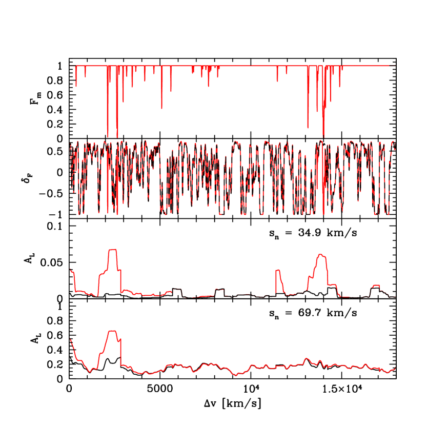
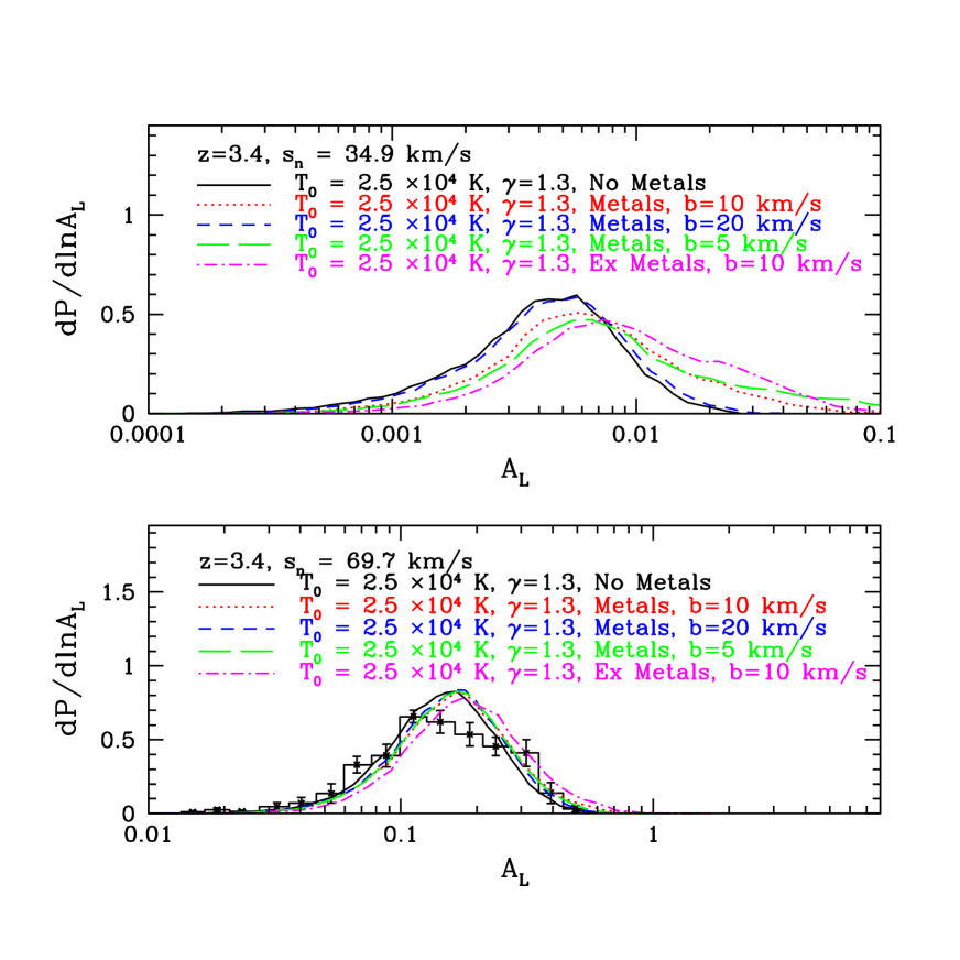
We have generated mock metal absorption lines according to the above prescription, and added them to simulated Ly-$\alpha$ forest spectra at $z=2.2,3.0,3.4$ and $4.2$. A typical example sightline at $z=3.4$ is shown in Figure 31, assuming $b=10$ km/s and $T_{0}=2.5\times 10^{4}$ K, $\gamma=1.3$. This illustrates a few key qualitative features regarding metal line contamination, and its impact on the wavelet amplitudes. The first feature is that our mock metal absorbers do lead to prominent peaks in the wavelet amplitudes, similar to the peaks observed and associated with metal absorbers in our observational data (§3.2). The next feature one notices is the considerably larger impact of metal absorbers on the smaller smoothing scale, again consistent with our previous findings from observational data. In some cases there are peaks in the wavelet amplitude on the smaller smoothing scale that are entirely absent at larger smoothing scale. For example, the metal line absorbers beyond $\Delta v\gtrsim 10,000$ km/s in Figure 31 produce peaks in the wavelet amplitude only on the smaller filtering scale. There are also cases where metal line absorbers lead to peaks for both filters (e.g. the lines near $\Delta v\sim 2,000$ km/s). In these cases, the fractional boost in wavelet amplitude from the metal lines is larger for the smaller smoothing scale filter. The metal lines are typically narrower than the HI lines, and the fractional contamination is hence significantly larger on small scales. Finally, a metal line that lands on a pixel where there is already significant Ly-$\alpha$ absorption is obviously irrelevant. We find many examples from the mock spectra of strong, narrow metal lines that happen to overlap strong Ly-$\alpha$ lines, and have little impact as a result. The strong increase in the mean absorption with redshift, and the corresponding boost in the amplitude of fluctuations in the forest, result in significantly less contamination towards high redshift. For example, in our simulated models the fractional impact of metals on the mean wavelet amplitude (for $s_{n}=34.9$ km/s) is $7$ times larger at $z=2.2$ than it is at $z=4.2$.

In order to provide a more quantitative measure of the impact of metal lines on wavelet amplitude measurements, we measure the wavelet PDF from $1,000$ mock spectra with added metal lines. Examples at $z=3.4$ are shown in Figure 32. By comparing the top and bottom panels, one can see that the metal lines generally have a much larger impact on the smaller filtering scale. At $s_{n}=34.9$ km/s, for $b=5$ and $10$ km/s, the mean wavelet amplitude is shifted significantly, and the PDF develops a long tail towards high wavelet amplitudes. There is relatively little impact for lines with larger b-parameters, as demonstrated by the $b=20$ km/s curve, but most observed CIV lines have smaller b-parameters: $b=20$ km/s is really at the upper end of the observed CIV linewidths (Boksenberg et al. 2003). We have also generated a more extreme model, with $6$ independent sets of CIV-like lines. Even this model produces only a small shift in the wavelet PDF on the large smoothing scale. Although our model for metal lines is rather crude, we expect fairly small shifts in the wavelet amplitudes on the larger smoothing scale, especially in the higher redshift bins.

Appendix C: Convergence with Simulation Resolution and Boxsize

In this section we assess the convergence of the simulated wavelet PDFs with increasing simulation resolution and boxsize. It is relatively challenging to obtain fully converged results in Ly-$\alpha$ forest simulations. On the one-hand, one needs to simulate a large volume to: compare simulations with large scale flux power spectrum measurements (if desired), to sample a representative fraction of the Universe, to capture the cascade of power from large to small scales, and to simulate peculiar velocity fields, which are coherent on rather large scales. On the other hand, high mass and spatial resolution at the level of tens of $kpc$ (in regions of low to moderate overdensity) are required to fully resolve the filtering (Gnedin & Hui 1998) and thermal broadening scales.

In order to examine the convergence of the wavelet PDFs with simulation volume, we ran a set of cosmological SPH simulations with fixed mass and spatial resolution, yet increasing boxsize. Specifically, we ran simulations with boxsize $L_{b}$ and particle number $N_{p}$ of $(L_{b},N_{p})=(12.5\rm{Mpc}/h,2\times 256^{3})$, $(25\rm{Mpc}/h,2\times 512^{3})$, and $(50\rm{Mpc}/h,2\times 1024^{3})$. To isolate resolution effects, we ran a sequence of fixed boxsize, increasing particle number simulations with $(L_{b},N_{p})=(25\rm{Mpc}/h,2\times 256^{3})$, $(25\rm{Mpc}/h,2\times 512^{3})$, and $(25\rm{Mpc}/h,2\times 1024^{3})$. In each simulation the force softening was set to $1/20$th of the mean inter-particle spacing. In general, the initial conditions in each of the fixed boxsize simulations are drawn from the same random number seeds, so that the Fourier modes of the initial displacement field are identical (for the wavenumbers common to each pair of simulations). Owing to imperfect planning, however, the highest resolution simulation with $N_{p}=2\times 1024^{3}$ particles was run with different initial conditions, and so there are random differences between this simulation and the lower resolution realizations, in addition to any systematic dependence on resolution. Given that the random seed-to-seed fluctuations are fairly small, and that are results are fairly well converged, we have not rerun the (faster) lower resolution simulations with initial conditions that match the highest resolution run.

Figure 33.— Wavelet amplitude PDF as a function of boxsize at $z=4$. The curves show the wavelet amplitude PDF at fixed mass resolution for simulations of varying boxsize for each of two thermal history models. The set of curves to the left, centered near $A_{L}=0.02$ has $(T_{0},\gamma)=(2\times 10^{4}K,1.3)$, while those on the right have $(T_{0},\gamma)=(1\times 10^{4}K,1.6)$.

Figure 34.— Wavelet amplitude PDF as a function of boxsize at $z=3$. Identical to Figure 33, except at $z=3$.

Figure 35.— Wavelet amplitude PDF as a function of boxsize at $z=2$. Identical to Figure 33 and Figure 35, except at $z=2$.

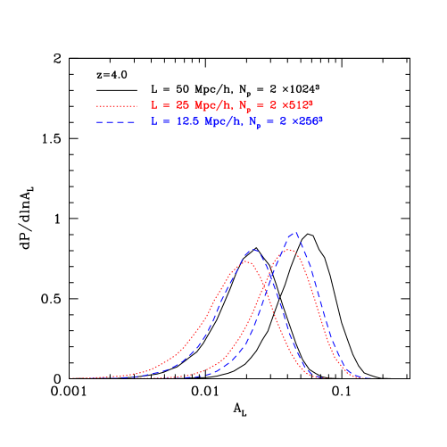
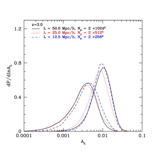
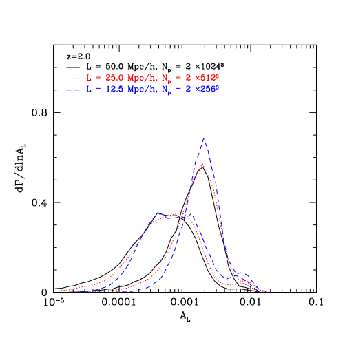
In order to test how the convergence depends on redshift (mostly owing to evolution in the mean transmitted flux) we examine simulation outputs at $z=2,3$, and $4$. We re-adjust the intensity of the ionizing background in each simulation to match a given (averaged over all sightlines) mean transmitted flux. At $z=3$, we assume a mean transmitted flux of $\langle F\rangle=0.680$. For the tests here, we adopt $\langle F\rangle=0.849$ at $z=2$, and $\langle F\rangle=0.393$ at $z=4$. We assume a perfect temperature density relation when incorporating thermal broadening in the mock quasar spectra. To test whether the convergence depends on the assumed model for the thermal state of the IGM, we consider two temperature-density relations: $(T_{0},\gamma)=(2\times 10^{4}K,\gamma=1.3)$ and $(T_{0},\gamma=1\times 10^{4}K,\gamma=1.6)$. In each case we adopt a small-scale smoothing of $s_{n}=34.9$ km/s and a large scale smoothing of $L=1,000$ km/s (see §2.3). In the text we consider $s_{n}=69.7$ km/s as well as $s_{n}=34.9$ km/s, but the resolution requirements are more stringent on the smaller of these scales, and so we consider it throughout this convergence study.

The results of the boxsize convergence test are shown in Figures 33-35. The convergence with simulation boxsize is generally encouraging. In fact, the wavelet PDFs from the rather small $L_{b}=12.5$ Mpc/$h$ box are similar to those in the larger $L_{b}=25$ Mpc/$h$ and $L_{b}=50$ Mpc/$h$ volumes. The $z=2$ results, however, suggest that the $L_{b}=12.5$ Mpc/$h$ box is a bit small: the wavelet PDF looks systematically narrow compared to the PDF in the larger volume simulations, although the differences are fairly small. It is not particularly surprising that this small volume run is inadequate at $z=2$, even for the relatively undemanding task of characterizing the distribution of small-scale power. For one, the amplitude of the linear power spectrum at the fundamental mode of this simulation box is $\Delta^{2}(k_{F})\sim 0.4$ in our adopted cosmology at this redshift, and so one does expect to start seeing systematic errors from missing large scale modes. In some of the $z=3$ and $z=4$ models the trend with boxsize appears to be non-monotonic. This may suggest that some of the differences are random, rather than systematic: i.e., a different choice of random number seed in the initial conditions can shift the PDF around a little bit in the smaller volumes. This scatter can be reduced by running several different realizations of each model and averaging, but the effects are small and so we do not pursue this here. It may also be that some of the non-monotonic trends result from two competing systematic effects. For present purposes, bear in mind that our main goal is to distinguish hotter $T_{0}\sim 2\times 10^{4}K,\gamma=1.3$ models from cooler $T_{0}\sim 1\times 10^{4}K,\gamma=1.6$ models: the differences between simulations of different boxsize are mostly quite small compared to the model differences. The one possible exception appears to be for the cooler model at $z=4$, where the peak of the PDF appears at surprisingly large amplitude in the large volume simulation, although the boxsize shift is still relatively small compared to the difference between the hot and cold models. Since we focus on small-scale fluctuations in this paper, and we find that the resolution requirements are fairly stringent at high redshift (see below), we sacrifice simulation volume slightly for resolution and adopt $L=25$ Mpc/$h$ as our fiducial boxsize.

Figure 36.— Wavelet amplitude PDF as a function of resolution at $z=4$. The curves show the wavelet amplitude PDF at fixed boxsize in simulations of varying mass and spatial resolution for each of two thermal history models. The set of curves to the left have $(T_{0},\gamma)=(2\times 10^{4}K,1.3)$, while those on the right have $(T_{0},\gamma)=(1\times 10^{4}K,1.6)$.

Figure 37.— Wavelet amplitude PDF as a function of resolution at $z=3$. Identical to Figure 36, except at $z=3$.

Figure 38.— Wavelet amplitude PDF as a function of resolution at $z=2$. Identical to Figure 36 and Figure 38, except at $z=2$.

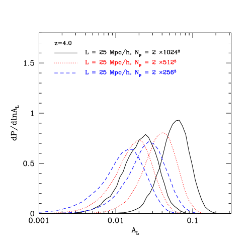
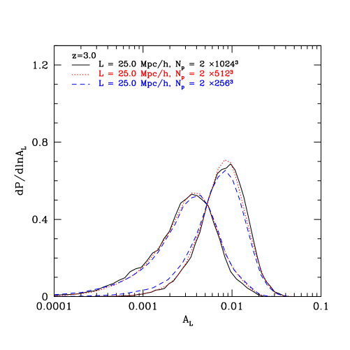
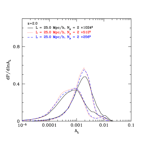
Next we show the results of varying the spatial and mass resolution at fixed simulation volume (Figures 36-38). At $z=2$ and $z=3$, the results of the $N_{p}=2\times 256^{3}$, $L_{b}=25$ Mpc/$h$ and the $N_{p}=2\times 512^{3}$, $L_{b}=25$ Mpc/$h$ simulations are quite similar. This gives us confidence that even the $N_{p}=2\times 512^{3}$, $L_{b}=25$ Mpc/$h$ simulation is adequately converged at these redshifts for measurements of the wavelet PDF. At $z=4$, however, there are noticeable differences, suggesting that higher spatial resolution is required. Note that the convergence with resolution is better for the hotter model. Since the data appear to favor this model over the cooler model, its convergence properties may be more relevant. It is clear, however, that resolution requirements are rather stringent at high redshift and so we use the $L_{b}=25$ Mpc/$h$, $N_{p}=2\times 1024^{3}$ simulation as our main simulation run throughout. Note also that any bias from limited simulation resolution causes us to systematically underestimate the temperature of the IGM, and strengthens the argument for a hot IGM.

Table 1The probability distribution of $A_{L}$ at $\bar{z}=4.2$.

Bin No.	$A_{L}$	$dP/dlnA_{L}$	$\sigma_{P}$
1	0.121E+00	0.102E-01	0.958E-02
2	0.164E+00	0.511E-01	0.421E-01
3	0.220E+00	0.117E+00	0.913E-01
4	0.285E+00	0.292E+00	0.145E+00
5	0.396E+00	0.395E+00	0.598E-01
6	0.516E+00	0.736E+00	0.124E+00
7	0.726E+00	0.850E+00	0.195E+00
8	0.943E+00	0.652E+00	0.135E+00
9	0.124E+01	0.131E+00	0.631E-01
10	0.167E+01	0.362E-01	0.281E-01

Note. — Here the Morlet filter scale is $s_{n}=69.7$ km/s. The first column is the bin number, the second column is the average wavelet amplitude in the bin, the third column is the differential PDF (per ln $A_{L}$) in the bin, and the fourth column is the $1-\sigma$ error on the differential PDF. The measurements have not been corrected for metal line contamination.

Table 2The probability distribution of $A_{L}$ at $\bar{z}=3.4$.

Bin No.	$A_{L}$	$dP/dlnA_{L}$	$\sigma_{P}$
1	0.155E-01	0.108E-01	0.800E-02
2	0.207E-01	0.226E-01	0.113E-01
3	0.334E-01	0.420E-01	0.223E-01
4	0.493E-01	0.115E+00	0.504E-01
5	0.710E-01	0.321E+00	0.452E-01
6	0.108E+00	0.601E+00	0.526E-01
7	0.156E+00	0.577E+00	0.641E-01
8	0.231E+00	0.478E+00	0.601E-01
9	0.335E+00	0.289E+00	0.835E-01
10	0.466E+00	0.404E-01	0.220E-01

Note. — Similar to Table 1 except at $\bar{z}=3.4$.

Table 3The probability distribution of $A_{L}$ at $\bar{z}=3.0$.

Bin No.	$A_{L}$	$dP/dlnA_{L}$	$\sigma_{P}$
1	0.498E-02	0.591E-02	0.617E-02
2	0.825E-02	0.351E-01	0.339E-01
3	0.129E-01	0.271E-01	0.146E-01
4	0.190E-01	0.897E-01	0.474E-01
5	0.322E-01	0.196E+00	0.495E-01
6	0.523E-01	0.394E+00	0.708E-01
7	0.800E-01	0.618E+00	0.858E-01
8	0.129E+00	0.509E+00	0.970E-01
9	0.202E+00	0.214E+00	0.650E-01
10	0.310E+00	0.159E-01	0.166E-01

Note. — Similar to Table 1 except corrected for metal line contamination, and at $\bar{z}=3.0$.

Table 4The probability distribution of $A_{L}$ at $\bar{z}=2.6$.

Bin No.	$A_{L}$	$dP/dlnA_{L}$	$\sigma_{P}$
1	0.135E-02	0.315E-02	0.327E-02
2	0.221E-02	0.159E-01	0.165E-01
3	0.445E-02	0.188E-01	0.151E-01
4	0.786E-02	0.523E-01	0.195E-01
5	0.149E-01	0.887E-01	0.418E-01
6	0.242E-01	0.126E+00	0.494E-01
7	0.479E-01	0.367E+00	0.579E-01
8	0.829E-01	0.595E+00	0.832E-01
9	0.142E+00	0.328E+00	0.578E-01
10	0.237E+00	0.764E-01	0.427E-01

Note. — Similar to Table 3 except at $\bar{z}=2.6$.

Table 5The probability distribution of $A_{L}$ at $\bar{z}=2.2$.

Bin No.	$A_{L}$	$dP/dlnA_{L}$	$\sigma_{P}$
1	0.846E-03	0.154E-01	0.160E-01
2	0.129E-02	0.331E-01	0.246E-01
3	0.230E-02	0.605E-01	0.304E-01
4	0.464E-02	0.129E+00	0.620E-01
5	0.834E-02	0.191E+00	0.706E-01
6	0.154E-01	0.149E+00	0.511E-01
7	0.285E-01	0.248E+00	0.567E-01
8	0.507E-01	0.554E+00	0.749E-01
9	0.820E-01	0.216E+00	0.758E-01
10	0.150E+00	0.531E-01	0.399E-01

Note. — Similar to Table 3 except at $\bar{z}=2.2$.

References

- (1) Abel, T., & Haehnelt, M. G. 1999, ApJL, 520, 13
- (2) Becker, G. D., Rauch, M., & Sargent, W. L. W. 2007, ApJ, 662, 72
- (3) Boksenberg, A., Sargent, W. L. W., & Rauch, M. 2003, astro-ph/0307557
- (4) Bolton, J. S., Viel, M., Kim, T.-S., Haehnelt, M. G., & Carswell, R. F. 2008, MNRAS, 386, 1131
- (5) Bolton, J. S., Oh, S. P., & Furlanetto, S. R. 2009, MNRAS submitted, arXiv:0807.2447
- (6) Bolton, J. S., & Becker, G. D. 2009, MNRAS in press, arXiv:0906.2861
- (7) Cen, R., McDonald, P., Trac, H., & Loeb, A. 2009, ApJL submitted, arXiv:0907.0735
- (8) Croft, R. A. C., Weinberg, D. H., Katz, N., & Hernquist, L. 1998, ApJ, 495, 44
- (9) Croft, R. A. C., Weinberg, D. H., Bolte, M., Burles, S., Hernquist, L., Katz, N., Kirkman, D. & Tytler, D. 2002, ApJ, 581, 20
- (10) Dall’Aglio, A., Wisotzki, L., & Worseck, G. 2008, A & A, 491, 465
- (11) Davé, R., Hernquist, L., Katz, N., & Weinberg, D.H. 1999, ApJ, 511, 521
- (12) Dijkstra, M., Lidz, A., & Hui, L. 2004, ApJ, 605, 7
- (13) Dixon, K. L., & Furlanetto, S. R. 2009, ApJ submitted, arXiv: 0906.4116
- (14) Eisenstein, D. J., & Hu, W. 1999, ApJ, 511, 5
- (15) Faucher-Giguère, C.-A., Lidz, A., Hernquist, L., & Zaldarriaga, M. 2008a, ApJ, 688, 85
- (16) Faucher-Giguère, C.-A., Prochaska, J. X., Lidz, A., Hernquist, L., & Zaldarriaga, M. 2008b, ApJ, 681, 831
- (17) Faucher-Giguère, C.-A., Lidz, A., Zaldarriaga, M., & Hernquist, L. 2009, ApJ submitted, arXiv:0901.4554
- (18) Furlanetto, S. R. 2008, ApJ submitted, arXiv:0812.3411
- (19) Furlanetto, S. R., & Oh, S. P. 2008, ApJ, 681, 1
- (20) Furlanetto, S. R., & Oh, S. P. 2009, ApJ submitted, arXiv:0901.1888
- (21) Gnedin, N. Y, & Hui, L. 1998, MNRAS, 296, 44
- (22) Haardt, F., & Madau, P. 1996, ApJ, 461, 20
- Hernquist et al. (1996) Hernquist, L., Katz, N., Weinberg, D. H., & Miralda-Escudé, J., 1996, ApJ 457, L51
- (24) Hopkins, P. F., Richards, G. T., & Hernquist, L. 2007, ApJ 654, 731
- Hui & Gnedin (1997) Hui, L. & Gnedin, N. Y., 1997, MNRAS 292, 27
- (26) Hui, L., Burles, S., Seljak, U., Rutledge, R., Magnier, E., & Tytler, D. 2001, ApJ, 552, 15
- (27) Hui, L. & Haiman, Z. 2003, ApJ, 596, 9
- (28) Kaiser, N., & Peacock, J. A. 1991, ApJ, 379, 482
- (29) Katz, N., Weinberg, D.H., Hernquist, L., & Miralda-Escudé, J., 1996, ApJ, 457, L57
- (30) Katz, N., Weinberg, D.H., & Hernquist, L. 1996a, ApJS, 105, 19
- (31) Kim, T. S., Viel, M., Haehnelt, M. G., Carswell, R. F., & Cristiani, S. 2004, MNRAS, 347, 355
- (32) Komatsu, E. et al. 2009, ApJS, 180, 330
- (33) Lai, K., Lidz, A., Hernquist, L., & Zaldarriaga, M. 2006, ApJ, 644, 61
- (34) Lidz, A., Heitmann, K., Hui, L., Habib, S., Rauch, M., & Sargent, W. L. W., 2006, ApJ, 638, 27
- (35) Lidz, A., McQuinn, M., Zaldarriaga, M., Hernquist, L., & Dutta, S. 2007, ApJ, 670, 39
- (36) Madau, P., Haardt, F., & Rees, M. J. 1999, ApJ, 514, 648
- (37) McDonald, P., Miralda-Escudé, J., Rauch, M., Sargent, W. L. W., Barlow, T. A., & Cen, R., 2001, ApJ, 562, 52
- (38) McDonald, P., et al. 2006, ApJS, 163, 80
- (39) McQuinn, M., Lidz, A., Zaldarriaga, M., Hernquist, L., Hopkins, P. F., Dutta, S., & Faucher-Giguère, C. A. 2008, ApJ in press, arXiv:0807.2799
- (40) McQuinn, M. 2009, ApJL submitted, arXiv:0905.0481
- (41) Miralda-Escudé, J. & Rees, M. J. 1994, MNRAS, 266, 343
- (42) Miralda-Escudé, J., Cen, R., Ostriker, J. P., Rauch, M., 1996, ApJ, 471, 582
- (43) Paschos, P., Norman, M. L., Bordner, J. O., & Harkness, R. 2007, arXiv:0711.1904
- (44) Ricotti, M., Gnedin, N. Y., & Shull, M. J., 2000, ApJ, 534, 41
- (45) Scannapieco, E., Pichon, C., Aracil, B., Petitjean, P., Thacker, R. J., Pogosyan, D., Bergeron, J., & Couchman, H. M. P. 2006, MNRAS, 366, 1118
- (46) Schaye, J., Theuns, T., Rauch, M., Efstathiou, G., & Sargent, W. L. W. 2000, MNRAS, 318, 817
- (47) Schaye, J., Aguirre, A., Kim, T.-S., Theuns, T., Rauch, M., & Sargent, W. L. W. 2003, ApJ, 596, 768
- (48) Seljak, U., Slosar, A., & McDonald, P. 2006, JCAP, 10, 14
- (49) Smette, A., Heap, S. R., Williger, G. M., Tripp, T. M., Jenkins, E. B., & Songaila, A. 2002, ApJ, 564, 542
- (50) Springel, V. & Hernquist, L. 2003, MNRAS, 339, 312
- (51) Springel, V. 2005, MNRAS, 364, 1105
- (52) Syphers, D., Anderson, S. F., Zheng, W., Haggard, D., Meiksin, A., Chiu, K., Hogan, C., Schneider, D. P., & York, D. G. 2009, ApJ, 690, 1181
- (53) Theuns, T., & Zaroubi, S. 2000, MNRAS, 317, 989
- (54) Theuns, T., Schaye, J., Zaroubi, S., Kim, T.-S., Tzanavaris, P., & Carswell, B. 2002a, ApJL, 567, L103
- (55) Theuns, T., Zaroubi, S., Kim, T.-S., Tzanavaris, P., & Carswell, R. F. 2002b, MNRAS, 332, 367
- (56) Tittley, E. R., & Meiksin, A., 2007, MNRAS, 380, 1369
- (57) Trac, H., Cen, R., & Loeb, A., 2008, ApJL, 689, 81
- (58) Viel, M., Haehnelt, M. G., & Springel, V. 2004, MNRAS, 354, 684
- (59) Viel, M., & Haehnelt, M. G. 2006, MNRAS, 365, 231
- (60) Viel, M., Bolton, J. S., & Haehnelt, M. G. 2009, MNRAS letters in press, arXiv:0907.2927
- (61) Weinberg, D. H., Hernquist, L., Katz, N., Croft, R. A. C., & Miralda-Escudé, J. 1998, in Proc. of the 13th IAP Colloquium, Structure and Evolution of the IGM from QSO Absorption Line Systems, eds. P. Petitjean & S. Charlot, Nouvelles Frontieres, Paris, 1998
- (62) Zaldarriaga, M., Hui, L., & Tegmark, M., 2001, ApJ, 557, 519
- (63) Zaldarriaga, M. 2002, ApJ, 564, 153