Parametrization dependence and $\mathbf{\Delta\chi^{2}}$ in parton distribution fitting

Abstract

Parton distribution functions, which describe probability densities of quarks and gluons in the proton, are essential for interpreting the data from high energy hadron colliders. The parton distributions are measured by approximating them with functional forms that contain many adjustable parameters, which are determined by fitting a wide variety of experimental data. This paper examines the uncertainty that arises from choosing the form of parametrization, and shows how that uncertainty can be reduced using a technique based on Chebyshev polynomials.

I Introduction

Interpreting the data from high energy hadron colliders such as the Tevatron and LHC relies on parton distribution functions (PDFs), which describe the probability densities for quarks and gluons in the proton as a function of lightcone momentum fraction $x$ and QCD factorization scale $\mu$. In current practice CT09 ; CT10 ; MSTW08 ; NNPDF , the PDFs are measured by parametrizing them at a low scale $\mu_{0}$, using functional forms in $x$ that contain many adjustable parameters. The PDFs at higher $\mu$ are calculated using QCD renormalization group equations, and the best-fit parameter values are found through a “global analysis,” in which data from a variety of experiments are simultaneously fitted by minimizing a $\chi^{2}$ measure of fit quality.

In the Hessian Hessian and Lagrange multiplier Lagrange methods, the uncertainty range of the PDFs is estimated by accepting all fits for which $\chi^{2}$ is not more than some fixed constant $\Delta\chi^{2}$ above the best-fit value. Traditionally, $\Delta\chi^{2}=100$ cteq66 or $\Delta\chi^{2}=50$ MRST2004 have been used to estimate the 90% confidence range. When these “large” $\Delta\chi^{2}$ values are used, weight factors or penalties may be included in the definition of the goodness-of-fit measure, to maintain an adequate fit to every individual data set CT09 ; or the uncertainty range along each eigenvector direction in the Hessian method can instead be estimated as the range where the fit to every experiment is acceptable MSTW08 . Large $\Delta\chi^{2}$ tolerance has long been a source of controversy. Some groups HERA ; Alekhin reject it in favor of the $\Delta\chi^{2}=1$ for 68% confidence ($\Delta\chi^{2}=2.7$ for 90% confidence) that would be expected from Gaussian statistics; however, results presented in this paper provide renewed evidence that substantially larger values of $\Delta\chi^{2}$ are necessary.

A potential motivation for large $\Delta\chi^{2}$ is based on conflicts among the input data sets, which signal unknown systematic errors in the experiments, or important theoretical errors introduced, e.g., by our reliance on leading-twist NLO perturbation theory, with a specific treatment for heavy quarks. It makes sense to scale up the experimental errors—which is equivalent to raising $\Delta\chi^{2}$—to allow for such conflicts PDG . However, the conflicts among experiments were recently shown DSD ; Consistency to be fairly small: the measured discrepancies between each experiment and the collective implications from all of the others suggest a minimum $\Delta\chi^{2}\approx 10$ for 90% confidence, but supply no clear incentive for $\Delta\chi^{2}\approx 100$. This is supported also by results from the NNPDF method NNPDF , which finds conflicts among the data sets to be relatively small. It is also supported by the distribution of $\chi^{2}$ per data point for the individual data sets CT10 ; and by the observation that the average $\chi^{2}$ per data point in the global fit is close to 1, which suggests that the experimental errors are not drastically understated and that the theory treatment is adequate Lyons .

Another source of uncertainty in PDF determination is the parametrization dependence error, which comes from representing the PDFs at $\mu_{0}$, which are unknown continuous functions, by expressions that are only adjustable through a finite number of free parameters. In traditional practice, flexibility is added to the parametrizing functions one parameter at a time, until the resulting minimum $\chi^{2}$ ceases to decrease “significantly.” However, at whatever point one chooses to stop adding fitting parameters, further small decreases in $\chi^{2}$ remain possible. This aspect of the PDF problem, namely that the number of fitting parameters is not uniquely defined, can spoil the normal rules, such as $\Delta\chi^{2}=1$ for 68% confidence, which would otherwise follow from standard Gaussian statistics. This point is illustrated in Sec. II by two hypothetical examples.

A method that uses Chebyshev polynomials to dramatically increase the freedom of the parametrization, while maintaining an appropriate degree of smoothness in the resulting PDFs, is introduced in Sec. III. The Chebyshev method is applied to a typical PDF fit in Sec. IV. The method is further applied to the most recent CTEQ fit in Sec. V. Some aspects of the Chebyshev fit at large $x$ are discussed in Sec. VI. Conclusions are presented in Sec. VII.

II Hypothetical examples

Let $z$ represent a displacement from the minimum point in $\chi^{2}$, along some specific direction in the space of fitting parameters. It can be normalized such that

$$\chi^{2}\,=\,z^{2}\,+\,C$$ (1)

in the neighborhood of the minimum. The parameter $z$ could be any one of the eigenvector coefficients $z_{i}$ that are discussed in DSD or Consistency . Or by means of a suitable linear transformation $X=\alpha+\beta z$, $z$ could represent the prediction for some cross section $X$ that depends on the PDFs; or simply a PDF itself for some specific flavor, $x$, and $\mu$. According to standard statistics, Eq. (1) would imply $z=0\pm 1$ at 68% confidence and $0\pm 1.64$ at 90% confidence. If we assume instead—guided by Consistency —that $\Delta\chi^{2}=10$ for 90% confidence, we would expect $z=0\pm 3.16$ at that confidence. However, the following argument shows that the uncertainty range may in principle be much broader than that.

  

Figure 1: Contours of $\chi^{2}=3010$, $3020$, $3030,\dots$ in two hypothetical examples. In each case, the best fit has $\chi^{2}=3000$ at $z=10$. Meanwhile, if the fit is confined to $y=0$, the $\Delta\chi^{2}=10$ error limits appear to be $z=0\pm 3.16$, which is far too restrictive.

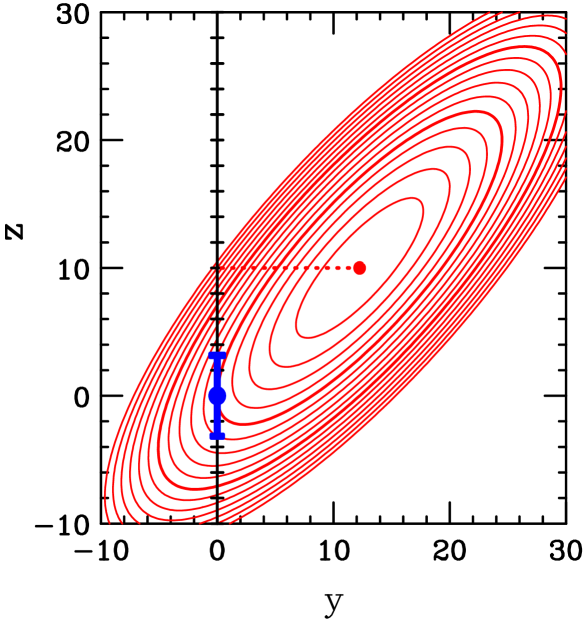
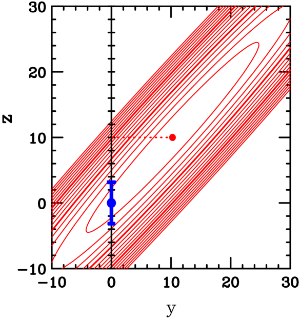
Suppose that, in order to reduce the dependence on the choice of parametrization, we introduce additional flexibility into the PDF model through a new parameter $y$, which is defined such that $\chi^{2}$ reduces to Eq. (1) at $y=0$. (To achieve a substantially improved fit, it will likely be necessary to increase the flexibility in more than one flavor, and therefore it will be necessary to introduce several new fitting parameters. The parameter $y$ thus represents displacement in a direction defined by some particular linear combination of several new and old parameters.)

Figure 1 shows two hypothetical contour plots for $\chi^{2}$ as a function of $y$ and $z$. The contour interval is 10. In each case, introducing the new parameter reveals that $z=10$ is a better estimate of the true value of $z$, so the prediction according to $y=0$, that $z=0\pm 3.16$ at 90% confidence, is inaccurate. In the scenario of the left panel, the additional freedom measured by $y$ has reduced the best-fit $\chi^{2}$ by $50$; while in the right panel, the reduction is only $5$—a change so small that one might easily have been content to mistakenly settle for $y=0$.

In the hypothetical examples of Fig. 1, $\Delta\chi^{2}=10$ yields an estimate of uncertainty for fits with $y=0$ that is far too narrow—even though in one case, the additional freedom only allows $\chi^{2}$ to be lowered by 5. Appendix 1 shows that the qualitative form of the dependence of $\chi^{2}$ on $y$ and $z$ shown in Fig. 1 arises rather generally, whenever additional freedom is introduced into the parametrizations. However, it remains to be seen whether such large quantitative changes actually arise in typical PDF fitting. A new parametrization method introduced in Sec. III will be used to answer that question in Secs. IV and V.

III Chebyshev parametrizations

In a recent typical PDF fit (CT09) CT09 , the gluon distribution was parametrized by

$$x\,g(x,\mu_{0})=a_{0}\,x^{a_{1}}\,(1-x)^{a_{2}}\,e^{p(x)}$$ (2)

where

$$p(x)=a_{3}\sqrt{x}\,+\,a_{4}x\,+\,a_{5}x^{2}\;.$$ (3)

The same form was used—with different parameters of course—for the valence quark distributions $u_{v}=u-\bar{u}$ and $d_{v}=d-\bar{d}$, except that $a_{3}$ was set to $0$ in $d_{v}$, because that distribution is less constrained by data.

To provide greater flexibility in the parametrization, it would be natural to replace $p(x)$ by a general polynomial in $\sqrt{x}\,$:

$$p(x)=\sum_{j=1}^{n}b_{j}\,x^{j/2}\;.$$ (4)

This form has several attractive features:

1. The power-law dependence at $x\to 0$, with subleading terms suppressed by additional powers of approximately $x^{0.5}$, is expected from Regge theory.

2. The power-law suppression in $(1-x)$ at $x\to 1$ is expected from spectator counting arguments.

3. The exponential form $e^{p(x)}$ allows for the possibility of a large ratio between the coefficients of the power-law behaviors at $x\to 0$ and $x\to 1$, without requiring large coefficients. It also conveniently guarantees that $g(x)$ is positive definite—although that could in principle be an unnecessarily strong assumption, since the $\overline{\mbox{MS}}$ parton distributions are not directly observable, so it is only required that predictions for all possible cross sections be positive.

4. Restricting the order $n$ of the polynomial in Eq. (4) can help to express the assumed smoothness of the parton distributions; although if $n$ is large, additional conditions must be imposed to prevent unacceptably rapid variations.

The constraints on smoothness and limiting behavior at $x\to 0$ and $x\to 1$ are important. For without them, the momentum sum rule

$$\sum_{a}\int_{0}^{1}f_{a}(x,\mu)\,x\,dx\,=\,1$$ (5)

and the valence quark number sum rules

$$\int_{0}^{1}u_{v}(x,\mu)\,dx\,=\,2\;,\qquad\int_{0}^{1}d_{v}(x,\mu)\,dx\,=\,1$$ (6)

would have no power, because mildly singular contributions near $x=1$ in (5) or near $x=0$ in (6) could make arbitrary contributions to those integrals, without otherwise affecting any predictions.

In past practice, only a small number of nonzero parameters $b_{j}$ have been retained in (4), as exemplified by the typical choice (3). The number of parameters can be increased to add flexibility, and thereby reduce the dependence on choice of parametrization. However, that quickly runs into a technical difficulty: as more fitting parameters are included, the numerical procedure to find the minimum of $\chi^{2}$ becomes unstable, with large coefficients and strong cancellations arising in $p(x)$. The resulting best fits, if they can be found at all, contain implausibly rapid variations in the PDFs as a function of $x$.

This technical difficulty can be overcome by a method based on Chebyshev polynomials. These polynomials have a long tradition in numerical analysis, although they have only recently begun to be applied to PDF studies Radescu . The Chebyshev polynomials are defined—and conveniently calculated—by recursion:

$$T_{0}(y) = 1\,,\quad T_{1}(y)=y$$

$$T_{n+1}(y) = 2yT_{n}(y)-T_{n-1}(y)\;.$$ (7)

Since $T_{j}(y)$ is a polynomial of order $j$ in $y$, the parametrization (4) can be rewritten as

$$p(x)=\sum_{j=1}^{n}c_{j}\,T_{j}(y)\;,$$ (8)

where $y=1-2\sqrt{x}$ conveniently maps the physical region $0<x<1$ to $\,-1<y<1\,$.

The parameters $c_{1},\dots,c_{n}$ are formally equivalent to the parameters $b_{1},\dots,b_{n}$; but they are more convenient for fitting, because the requirement for smoothness in the input PDFs forces the $c_{j}$ parameters to be reasonably small at large order $j$. This can be seen from the following property of the Chebyshev polynomials:

$$T_{j}(y)=\cos(j\theta)\quad\mbox{where}\quad y=\cos\theta\;.$$ (9)

With the mapping $y=1-2\sqrt{x}\,$, $T_{j}(y)$ has extreme values of $\pm 1$ at the endpoints and at $j-1$ points in the interior of the physical region $0<x<1\,$. Chebyshev polynomials of increasingly large $j$ thus model structure at an increasingly fine scale in $x$.

Because the Chebyshev method provides so much flexibility in the parametrized input forms, there is a danger that it will produce fits with an unreasonable amount of fine structure in their $x$ distributions—potentially lowering $\chi^{2}$ in a misleading way by producing fits that match some of the statistical fluctuations in the data. This difficulty can be overcome by defining an effective goodness-of-fit measure that is equal to the usual $\chi^{2}$ plus a penalty term that is based on a measure of the structure in the input distributions. A particular way to include this “soft constraint” is described in Appendix 2. (The method is a major improvement over a method used to enforce smoothness in a preliminary version of this paper, which was based solely on the magnitudes of the coefficients $c_{j}$.)

With the Chebyshev method, it becomes possible to produce fits with three to four times as many free parameters than were tractable in previous PDF fitting. The method is applied in the next section to examine the parametrization error in a traditional fit.

IV Fits using the Chebyshev method

Figure 2: Fractional uncertainty of gluon distribution, and $d$ and $u$ quark distributions, calculated at $\Delta\chi^{2}=10$ using the CTEQ6.6 form of parametrization with 22 parameters. Dashed curves are from a fit using the Chebyshev polynomial method with 71 parameters.

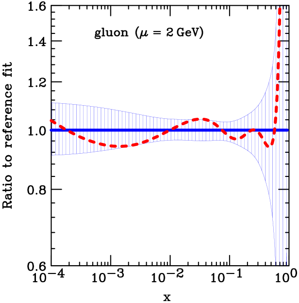
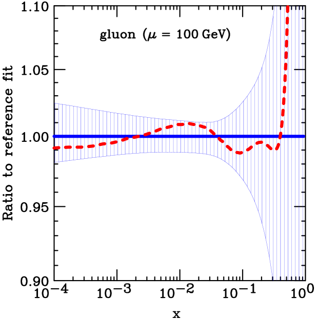
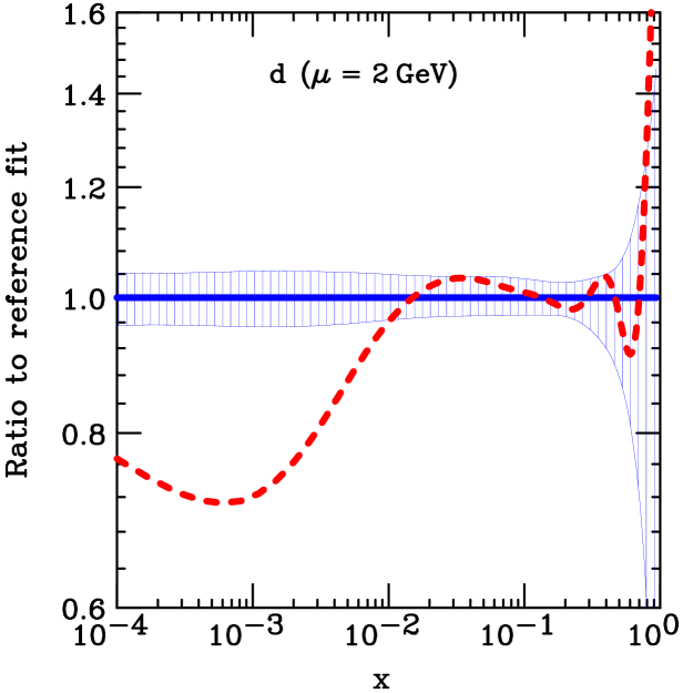
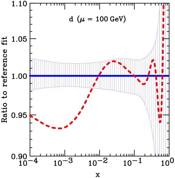
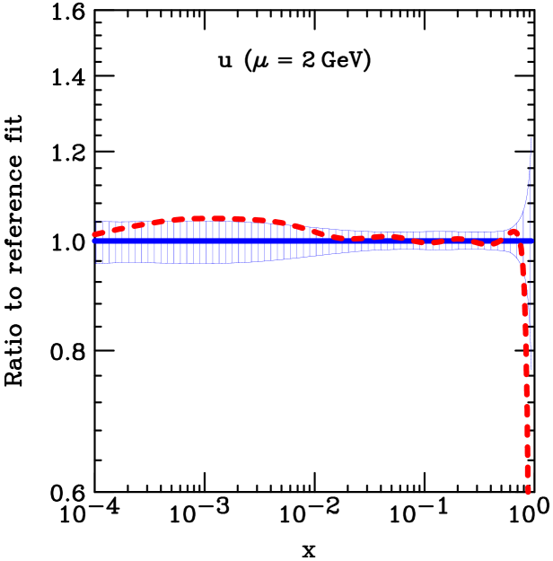
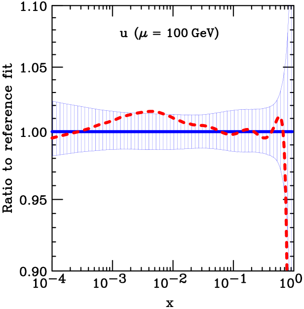
Figure 2 shows the fractional uncertainty obtained using the parametrization method of CTEQ6.6 cteq66 , which has 22 free parameters. The uncertainty limit is defined here by $\Delta\chi^{2}=10$, which is the range suggested by observed conflicts among the input data sets Consistency . The dashed curve shows the result of a fit using the Chebyshev method described in Appendix 2. This fit has 71 free parameters, and achieves a $\chi^{2}$ that is lower by $72\,$.

We see that introducing the more flexible parametrization has shifted the best-fit estimate of the PDFs by an amount that is in a number of places comparable to the previously estimated $\Delta\chi^{2}=10$ uncertainty. In some regions, namely at very large or very small $x$, the shift produced by the change in parametrization is much larger than the previous uncertainty estimate. These are regions where the available data provide little constraint on the PDFs, so their estimated uncertainty in the CTEQ6.6-style fit was artificially small due to the lack of flexibility in that parametrization. Other contemporary PDF fits use still less flexible parametrizations, which must underestimate the true uncertainty in those regions even more.

The fits shown in this section were made using a relatively crude method for imposing smoothness on the Chebyshev polynomial fits (based on limiting the magnitudes of the coefficients of those polynomials). As a consequence, substantial deviations from $u(x)\approx d(x)$ appear at $x$ as small as $10^{-4}$, in spite of the limiting condition $u(x)/d(x)\to 1$ at $x\to 0$ that is assumed in all of these fits. This can be seen in Fig. 2, where $u(x)$ and $d(x)$ are shifted quite differently from the CT10 reference fit, for which $u(x)\approx d(x)$ is a good approximation at small $x$. An improved method for imposing smoothness is used in the fits shown in the next section, and that restores the $u(x)\approx d(x)$ behavior at small $x$.

The second set of graphs in Fig. 2 shows that parametrization effects are still important at the relatively large scale of $\mu=100\,\mathrm{GeV}$. Hence they are an important source of uncertainty for many processes of interest at the Tevatron and LHC.

V Application to CT10

While this paper was being revised, an updated version of the CTEQ/TEA parton distribution analysis was completed. This CT10 CT10 analysis includes a number of improvements to the previous CTEQ6.6 cteq66 and CT09 CT09 analyses, and is now the most up-to-date of the CTEQ PDF fits. It is therefore interesting to examine the uncertainty caused by parametrization dependence in this new fit, using the Chebyshev technique.

Figure 3: Wide shaded regions show the fractional uncertainty of gluon, $d$-quark, and $u$-quark distributions at scales $\mu=2\,\mathrm{GeV}$ and $\mu=100\,\mathrm{GeV}$ according to CT10 (26 fitting parameters). Narrow shaded regions show the corresponding uncertainty defined by a simple $\Delta\chi^{2}=10$ criterion. The solid curves are from a fit using the Chebyshev polynomial method: this fit has 84 free parameters and its $\chi^{2}$ is lower than CT10 by $105$. The dashed and dotted curves show similar Chebyshev fits with different behaviors at large $x$.

Figure 4: Like Fig. 3, but displayed using linear scales to show the behavior at large $x$.

Figure 5: Absolute gluon and quark distributions with uncertainties from CT10 (solid), and the three Chebyshev fits from Figs. 3 and 4.

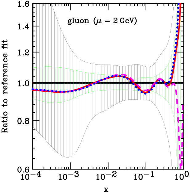
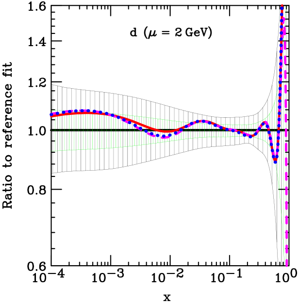
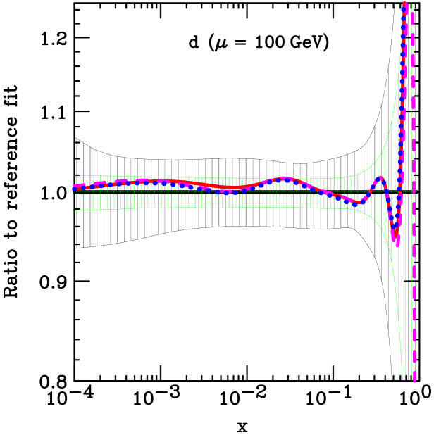
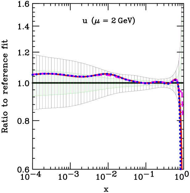
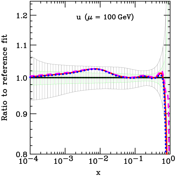
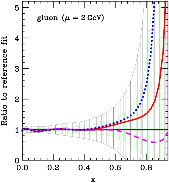
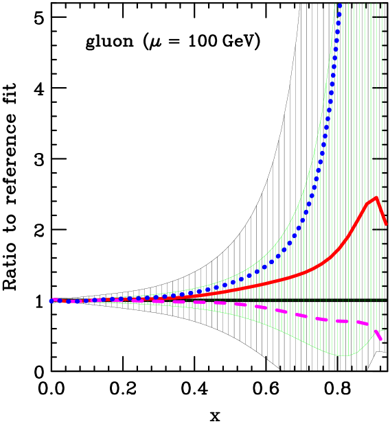
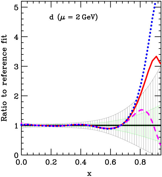
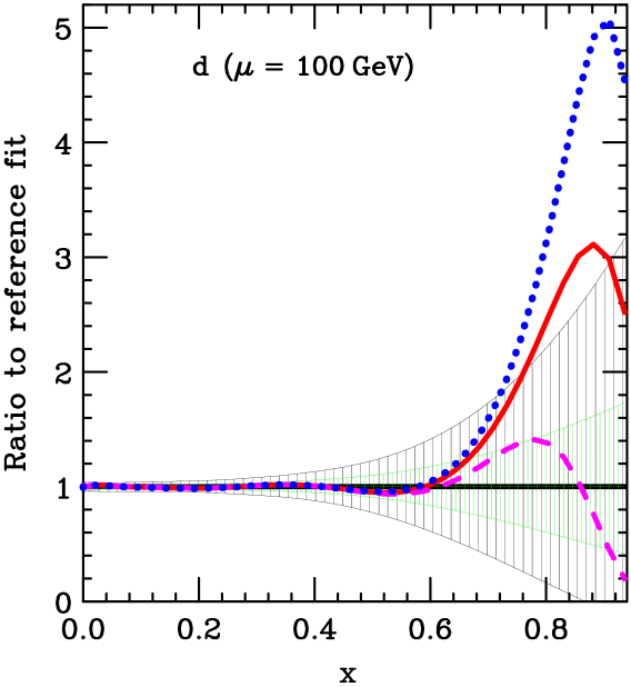
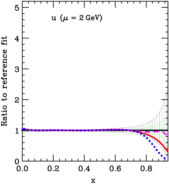
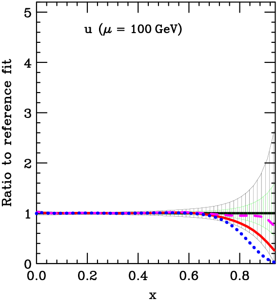
The wide shaded areas in Fig. 3 show the fractional uncertainty estimated at 90% confidence in CT10 CT10 , which employs a $\Delta\chi_{\mathrm{eff}}^{\,2}=100$ criterion on a goodness-of-fit measure $\chi_{\mathrm{eff}}^{\,2}$ that is defined as the sum of the usual $\chi^{2}$ plus supplemental “penalty” terms that are designed to force acceptable agreement to every data set over the entire allowed uncertainty range.

The narrow shaded areas correspond to an otherwise similar fit, in which the uncertainty criterion is replaced by the pure $\Delta\chi^{2}=10$ condition that was used in Sec. IV. The ratio of these uncertainties is seen to be roughly a factor of 2. It is not so large as the naive factor $\sqrt{100/10}=3.16$, because of the penalty terms included in the goodness-of-fit measure for CT10, and because quadratic dependence of $\chi^{2}$ on the fitting parameters holds only rather close to the minimum in $\chi^{2}$.

The solid curve in each plot shows the result of a fit that was carried out in exactly the same way as the CT10 best fit, except for using the Chebyshev parametrization described in Appendix 2. This fit has 84 free parameters—a few more than the Chebyshev fit of Sec. IV, because the simple CTEQ6.6 parametrization for strangeness was retained there. It achieves a $\chi^{2}$ that is lower than CT10 by 105. This fit demonstrates that parametrization dependence introduces an uncertainty in CT10 that in some places approaches its $\Delta\chi^{2}=100$ uncertainty estimate. This result is consistent with the fact that the actual reduction in $\chi^{2}$ is close to that value. This strong parametrization dependence can appear even in places where the fractional uncertainty is relatively small, such as in the $u$-quark distribution for $0.005\lesssim x\lesssim 0.010$ at $\mu=100\,\mathrm{GeV}$.

Figure 4 displays the same fits as Fig. 3, using linear scales to reveal the behavior at large $x$. The fractional uncertainty becomes large at very large $x$, because the available data provide little constraint there. In spite of the very large uncertainty found by CT10 in that region, the actual uncertainty is still larger, as is seen in the case of the $d$-quark distribution for $x\gtrsim 0.8$. This is not surprising, since the absence of experimental constraints implies that the behavior extracted at large $x$ is an extrapolation based mainly on the choice of parametrization. The solid curve in this figure is a best fit using the Chebyshev method, while the dotted and dashed curves were obtained by adding a small penalty to $\chi^{2}$ in the Chebyshev method to push the gluon and $d$ quark distributions up or down relative to the $u$ quark distribution at large $x$. These dotted and dashed fits have a $\chi^{2}$ that is only $5$ units higher than the Chebyshev best fit (and hence lower than CT10 by $100$). The very large difference between the dotted and dashed curves for the $d$-quark therefore corresponds to an uncertainty range of only $\Delta\chi^{2}=5$. The full $d$-quark uncertainty in the large-$x$ region must therefore be still much larger.

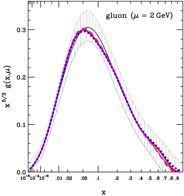
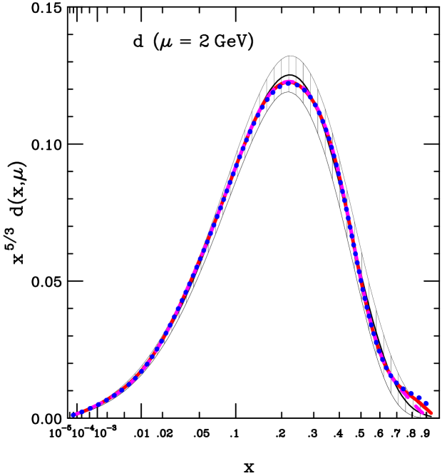
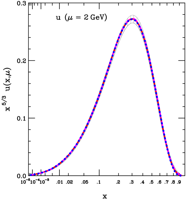
The flexibility of the Chebyshev parametrization is such that it could easily produce fits that contain unrealistically rapid variations in the PDFs as a function of $x$. A necessary aspect of Chebyshev fitting, as described in Appendix 2, is therefore to include a penalty in the function that measures goodness-of-fit, to suppress any unwarranted fine structure. Figure 5 shows the same results as in Figs. 3 and 4 except that this time the absolute $g$, $d$, and $u$ PDFs are shown, instead of their ratio to the CT10 best fit. (The horizontal axis $x^{1/3}$ is used here to display both large and small $x$; while the weight factor $x^{5/3}$ included in the vertical axis makes the area under each curve proportional to its contribution to the momentum sum rule.) This figure demonstrates that the method outlined in Appendix 2 to restrict the fits to functions that are reasonably smooth is successful. Further evidence of the smoothness of the Chebyshev fits can be seen in Figs. 6–8 of Sec. VI.

One might find the “shoulder” that appears in the central Chebyshev fit in Fig. 5 for the $d$-quark distribution at $x\gtrsim 0.8$—and perhaps the milder shoulder in $g(x)$ at $x\gtrsim 0.6$—to be unlikely features of nuclear structure. These features are certainly not required by the data, since the dashed fits which do not have them have a larger $\chi^{2}$ by only 5 units; but at present, there seems to be no strong theoretical basis to exclude them.

The Chebyshev best fit shown here has $\chi^{2}=2916$ for $2753$ data points. This is lower than the CT10 $\chi^{2}$ by $105\,$. Since the 90% confidence uncertainty in CT10 is estimated using a $\Delta\chi^{2}=100$ criterion (with modifications to require an acceptable fit to each individual data set), it is not surprising that the parametrization error we find for CT10 is comparable to the CT10 error estimate, except at extreme values of $x$. At very large $x$, where the PDFs are poorly determined, the uncertainty in CT10 needs to be expanded, as evidenced by Fig. 4.

A large part of the decrease in $\chi^{2}$ produced by the Chebyshev fit comes from the BCDMS $\mu p\to\mu X$ Benvenuti:1989rh ($-21$) and BCDMS $\mu d\to\mu X$ Benvenuti:1989fm ($-16$) experiments, which are particularly sensitive to $u$ and $d$ quark distributions at large $x$. Other important improvements in the fit are to the combined HERA-1 data set HERAcombined ($-17$), to the CDF run 2 inclusive jet measurement CDFjet ($-15$), and to the E866 Drell-Yan pp data Webb:2003ps ($-11$).

VI PDF behavior at large x

Figure 6: Quark ratio $d(x)/u(x)$ at scales $\mu=2\,\mathrm{GeV}$ and $\mu=100\,\mathrm{GeV}$. Shaded area is CT10 with uncertainty; curves are the same Chebyshev fits shown in Figs. 3–5.

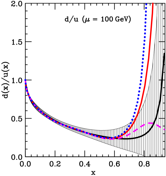
The parton distributions at large $x$ are not well constrained by data. For example, Fig. 6 shows a large uncertainty of the $d/u$ ratio at $x\gtrsim 0.8$. Recall that the dotted and dashed extreme curves shown here represent an increase in $\chi^{2}$ by only 5 units above the Chebyshev best fit, so the full uncertainty must be considerably larger than what is spanned by those curves.

Figure 7: Up quark (solid), down quark (dashed), and gluon (dotted) distributions at $\mu=1.3\,\mathrm{GeV}$ from CT10 (upper left), and the three Chebyshev fits, which have $\chi^{2}$ lower than CT10 by $105$, $100$, and $100$.

Figure 8: Like Fig. 7, but at scale $\mu=100\,\mathrm{GeV}$.

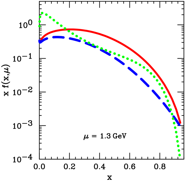
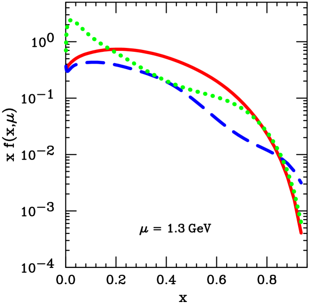
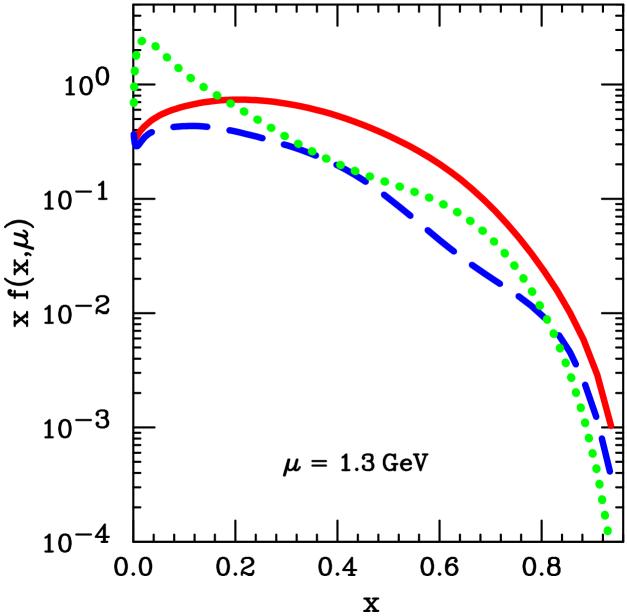
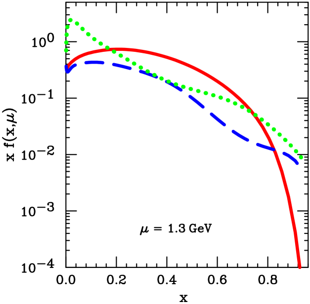
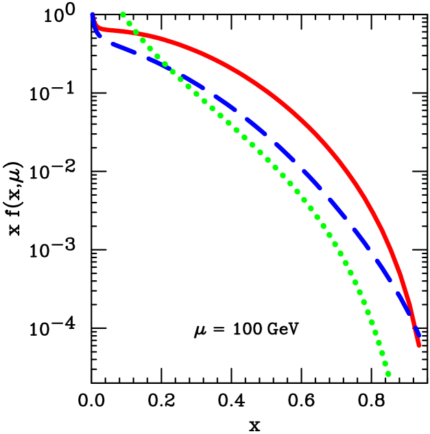
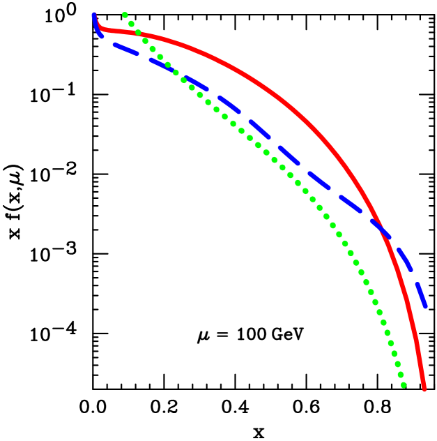
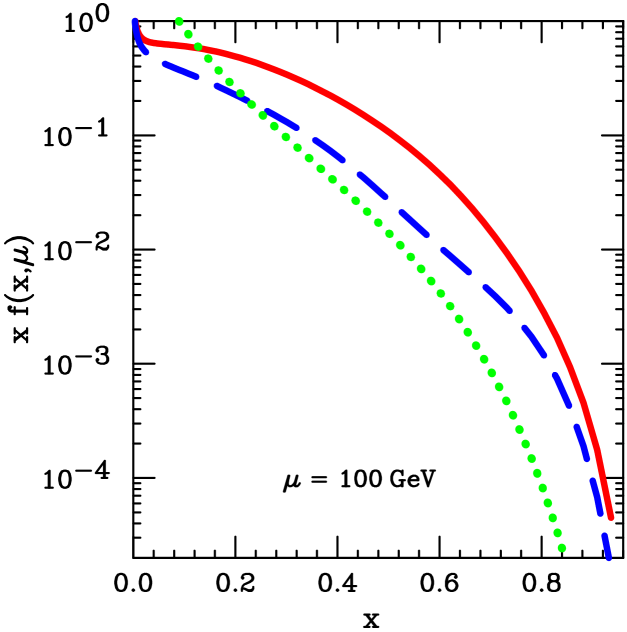
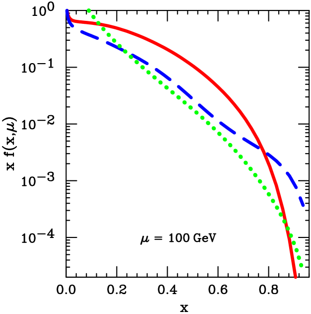
The large-$x$ behavior of the best fits for $u$, $d$, and $g$ at $\mu=1.3\,\mathrm{GeV}$ are compared directly in the first panel of Fig. 7 for CT10, and in the other three panels of Fig. 7 for the three Chebyshev fits that were shown in Figs. 3–6. We see that the intuitively expected order $u(x)\gg d(x)\gg g(x)$ in the limit $x\to 1$ is consistent with the fitting, since it appears in third panel of Fig. 7; but that this behavior is not required by it—e.g., $d(x)\gg u(x)\approx g(x)$ in the second panel, and $g(x)\approx d(x)\gg u(x)$ in the fourth panel. It is possible that theoretical ideas from nonperturbative physics such as $u(x)\gg d(x)\gg g(x)$ should be imposed to reduce the uncertainty of the fitting, by including a “soft constraint,” which would be implemented by adding an appropriately defined penalty to the effective $\chi^{2}$. However, all of these fits share the feature that $g(x)$ is comparable to or larger than $d(x)$ in the rather broad range $0.3\lesssim x\lesssim 0.8\,$. That valence-like behavior of the gluon poses an interesting challenge to be explained by hadron structure physics; but meanwhile, it demonstrates that naive expectations about the parton content of the proton can be unreliable. Figure 8 shows that the “natural” large-$x$ order $u(x)>d(x)>g(x)$ is restored by DGLAP evolution for factorization scales above $\mu=100\,\mathrm{GeV}$, except possibly at extremely large $x$.

VII Conclusion

Increasing the flexibility of the input parametrizations used in PDF analysis, using a method based on Chebyshev polynomials, has revealed a significant source of uncertainty in previous PDF determinations caused by parametrization dependence. As demonstrated in Figs. 3 and 5, the parametrization error is in many places as large as the uncertainty estimated, via $\Delta\chi^{2}=10$, on the basis of conflicts observed between the different data sets used in the analysis Consistency . At very large $x$, where the fractional PDF uncertainty is large, the parametrization error even becomes large compared to the modified $\Delta\chi^{2}=100$ uncertainty estimate used in CT10 CT10 , which was intended to represent a 90% confidence interval. These parametrization effects persist up to scales of $\mu=100\,\mathrm{GeV}$ and beyond, so they are significant for predictions of important background and discovery processes at the Tevatron and LHC.

The hypothetical example shown in the left panel of Fig. 1 raised the spectre of large possible shifts in a PDF fit when a new degree of freedom is included in the parametrization. As stated earlier, that degree of freedom must generally correspond to a linear combination of several new fitting parameters, since the reduction in $\chi^{2}$ depends on modifying more than one flavor in some particular correlated manner. We have seen that enhancing parametrization freedom by the Chebyshev method of Appendix 2 reduces $\chi^{2}$ for the fit to the CT10 data set by 105. That decrease is nearly equal to the tolerance criterion used to estimate the uncertainty in CT10, so it is not surprising that the corresponding changes in the PDFs can be comparable to the CT10 uncertainty estimate. This result lends support to the use of $\Delta\chi^{2}\sim 100$ in CT10, while suggesting the possibility that a somewhat tighter criterion could be used, once the Chebyshev-style parametrizations have been incorporated into the uncertainty analysis.

The right panel of Fig. 1 illustrates how large changes in the results could arise in principle even from a very modest decrease in $\chi^{2}$. Figure 4 shows that this can actually happen in practice, in regions where the results of fitting are dominated by parametrization assumptions because the data provide little constraint. In particular, the solid (red) curves in Figs. 4–6 show a best fit obtained using the Chebyshev method; while the dotted and dashed curves, which have rather different behavior at large $x$, are fits made by including mild constraints on the large-$x$ behavior. Those constraints are so mild that they increase the overall $\chi^{2}$ by only 5 units.

The parametrization effects discussed in this paper come from increasing the flexibility of the functional forms used to approximate the PDFs at the chosen starting scale $\mu_{0}$ for their evolution, without altering the various discrete assumptions that went into choosing those forms. For example, a much wider uncertainty range would be permitted for $\bar{d}(x)/\bar{u}(x)$ in Fig. 6 if the assumption $r=1$ were relaxed, where $r={\displaystyle\lim_{x\to 0}}(\bar{d}(x,\mu_{0})/\bar{u}(x,\mu_{0}))$. Indeed, the range $0.4<r<1.2$ would be permitted by an increase in $\chi^{2}$ as small as $\Delta\chi^{2}=5$. (The parameter $r$ is treated as a free parameter in the Alekhin2002 PDFs Alekhin : its value in the central fit is approximately $0.8\,$.) As a still more blatant example of these choices, all of the fits discussed here have $s(x,\mu)=\bar{s}(x,\mu)$ as a result of a simplifying assumption in the parametrization. Dropping that approximation would allow a very wide range of the asymmetry $(s(x)-\bar{s}(x))/(s(x)+\bar{s}(x))$.

In future analyses, it will be important to properly combine the parametrization uncertainty with the other sources of uncertainty that have previously been included in the Hessian method. A step in that direction could be made by using a very flexible parametrization such as the Chebyshev one to determine the best fit, but then to freeze enough of the parameters to make the usual Hessian method tractable. This would be an extension of the approach already used in MSTW MSTW08 and CTEQ Hessian fits, wherein one or two parameters for each flavor are frozen at their best-fit values before the Hessian eigenvector method is carried out. Once the parametrization error has been reduced by means of more flexible parametrizations, it should become possible to apply a tighter uncertainty criterion, e.g., comparable to the $\Delta\chi^{2}\approx 10$ for 90% confidence that is suggested by the observed level of consistency Consistency among input data sets.

An alternative method to avoid parametrization dependence is offered by the NNPDF approach NNPDF , in which the PDFs at $\mu_{0}$ are represented using a neural network model that contains a very large number of effective parameters. Broadly speaking, the uncertainties estimated in this way appear to be consistent with the results presented here. A more detailed comparison will require allowing for differences in assumptions about the nonperturbative hadronic physics, such as positivity of the input distributions. Attention will also have to be paid to the choice of assumptions about behaviors in the $x\to 0$ and $x\to 1$ limits, which are imposed in the NNPDF approach by “preprocessing exponents.” This will be undertaken in a future work.

Appendix 1: General form of $\chi^{2}$ near its minimum

This Appendix shows that the qualitative behavior of $\chi^{2}(y,z)$ hypothesized in Fig. 1 arises under rather general assumptions.

Let us assume as usual that $\chi^{2}$ can be approximated in the neighborhood of its minimum by Taylor series through second order. To find the uncertainty of a particular variable, we can assume by means of a linear transformation of that variable, that we are interested in the value of a parameter $z$ for which $\chi^{2}=z^{2}\,+\,C$ at $y=0$, as in Eq. (1). Now let $y$ represent an additional fitting parameter that was previously held fixed at $0$. By Taylor series, the expression for $\chi^{2}$ expands to become

$$\chi^{2}\,=\,z^{2}\,+\,y^{2}\,+\,2Azy\,+\,2By\,+\,C\,,$$ (10)

where the coefficient of $y^{2}$ was chosen to be $1$ without loss of generality, by scaling that variable. Equation (10) implies that the contours of constant $\chi^{2}$ are ellipses whose major and minor axes make an angle of $\pm 45^{\circ}$ with respect to the $y$ and $z$ axes, as in the specific examples of Fig. 1. The ratio of minor axis to major axis of the ellipse is $\sqrt{(1-|A|)/(1+|A|)}\,$, and $|A|<1$ is required, since $\chi^{2}$ must have a minimum. The minimum of $\chi^{2}$ occurs at

$$z_{0}=AB/(1-A^{2})\,,\quad y_{0}=-B/(1-A^{2})\;,$$ (11)

and its value there is

$$\chi_{0}^{\,2}\,=\,C\,-\,D\,,\;\mbox{where}\;D\,=\,B^{2}/(1-A^{2})\;.$$ (12)

Relative to the $y=0$ situation given by Eq. (1), introducing the additional parameter $y$ thus allows the best-fit $\chi^{2}$ to be lowered by $D$. At the same time, it demands that the uncertainty range for $z$ be extended at least far enough to include $z_{0}$, and hence demands $\Delta\chi^{2}>z_{0}^{\,2}\,$ in the $y=0$ model.

The hypothetical examples shown in Fig. 1 correspond to $A=B/5=-\,\sqrt{2/3}\,$ $\,\Rightarrow\,$ $(z_{0}=10$, $D=50$), and $A=2B=-\,\sqrt{20/21}\,$ $\,\Rightarrow\,$ ($z_{0}=10$, $D=5$).

Appendix 2: Details of a specific Chebyshev method

This Appendix describes a specific method that uses Chebyshev polynomials to parametrize the parton distributions at starting scale $\mu_{0}$, in a manner that allows great freedom in the functions, while maintaining their expected smoothness.

Each flavor is parametrized by the form (2), with $p(x)$ given by (8) with $y=1-2\sqrt{x}$. For the studies presented this paper, $n=12$ was used for each flavor. There are 6 flavors to be parametrized ($g$, $u_{v}$, $d_{v}$, $\bar{u}$, $\bar{d}$, and $\bar{s}$, with $s(x)=\bar{s}(x)$ assumed), so this leads to 72 fitting parameters.

To facilitate studying the effect of imposing constraints such as $\bar{d}(x)/\bar{u}(x)\to 1$ at $x\to 0$, instead of parametrizing $\bar{u}(x)$ and $\bar{d}(x)$ separately, the sum $\bar{u}(x)+\bar{d}(x)$ was parametrized in the manner described above for the other flavors, while the ratio $\bar{d}(x)/\bar{u}(x)$ was parametrized by

$$\bar{d}(x)/\bar{u}(x)\,=\,\exp\left(c_{0}\,+\,\sum_{j=1}^{13}c_{j}\,(T_{j}(y)-1)\,\right)\;.$$ (13)

This method provides freedom for $\bar{u}(x)$ and $\bar{d}(x)$ separately that is comparable to the great freedom for other flavors, while allowing the ratio $\bar{d}(x)/\bar{u}(x)$ in the limit $x\to 0$ to be controlled entirely by $c_{0}$. The value $c_{0}=0$ is used in the fits presented here, so that $\bar{d}(x)/\bar{u}(x)\to 1$ at $x\to 0$.

In future work, it might be preferable to include an additional factor of $(1-x)^{a_{2}}$ in $\bar{d}(x)/\bar{u}(x)$, to allow $\bar{d}(x)$ and $\bar{u}(x)$ to have different asymptotic behaviors at $x\to 1$. However, the dominance of the quark distributions by valence contributions at large $x$ means that this would be unlikely to affect the phenomenology. Similarly, one might prefer to include an additional factor of $x^{a_{1}}$ here, to allow $\bar{d}(x)$ and $\bar{u}(x)$ to have different limiting power laws at $x\to 0$. However, that would involve lifting the Regge assumption that $\bar{d}$, $\bar{u}$, and $\bar{s}$ all have the same small-$x$ power law behavior. It would also have little effect on the phenomenology, because we find that assuming an arbitrary constant limiting value for $\bar{d}(x)/\bar{u}(x)$ at $x\to 0$ results in a very large uncertainty in the value of that constant.

There are additional free parameters associated with the strange and sea quark momentum fractions and the $x^{a_{1}}$ and $(1-x)^{a_{2}}$ factors—with some of the $a_{1}$ parameters tied together by Regge theory. In all, the Chebyshev fits of Sec. V have 84 free parameters: $c_{1},\dots,c_{12}$ in Eq. (8) for $u_{v}$, $d_{v}$, $g$, $\bar{d}+\bar{u}$, and $\bar{s}$; $c_{1},\dots,c_{13}$ in Eq. (13) for $\bar{d}/\bar{u}$; $a_{2}$ in Eq. (2) for $u_{v}$, $d_{v}$, $g$, $\bar{d}+\bar{u}$, $\bar{s}$; $a_{1}$ in Eq. (2) for $u_{v}$, $g$, $\bar{d}+\bar{u}$, $\bar{s}$, with $u_{v}$ and $d_{v}$ values equal; $a_{0}$ in Eq. (2) for $\bar{d}+\bar{u}$, $\bar{s}$, with $a_{0}$ for $u_{v}$ and $d_{v}$ determined by the number sum rules (6) and for $g$ by the momentum sum rule (5).

To make a fair comparison with CTEQ6.6-style fits, the Chebyshev fits discussed in Sec. IV retained the same parametrization for $\bar{s}(x)$ as in CTEQ6.6 and require $\bar{d}(x)/\bar{u}(x)\to 1$ at $x\to 0$, leaving 71 free parameters for these fits.

The Chebyshev parametrizations used here have 3–4 times as many adjustable parameters as have been used in traditional PDF analyses. This provides sufficient flexibility to avoid the systematic error of “parametrization dependence,” but it also means that the parametrized forms can easily take on more fine structure in $x$ than is plausible in the nonperturbative physics that is being described. To avoid undesirable fine structure, we adopt a strategy of adding a penalty to the $\chi^{2}$ measure of fit quality, based on the amount of complexity in the fitting functions.

To construct a suitable penalty, let us observe that the classic form

$$f(x)=a_{0}\,x^{a_{1}}\,(1-x)^{a_{2}}\;,$$ (14)

which surely embodies the appropriate smoothness, has the property that

$$x\,(1-x)\,d(\ln f)/dx\,=\,a_{1}-(a_{1}+a_{2})x$$ (15)

is linear in $x$. Hence it is natural to define

$$\Phi_{a}(x)\,=\,x\,(1-x)\,d(\ln f_{a})/dx$$ (16)

for each flavor $a=u$, $d$, $\bar{u}$, $\bar{d}$, $s$, and $g$. The extent to which $\Phi_{a}(x)$ departs from a linear function is a good local measure of nonsmoothness, so we define

$$S_{a}\,=\,\int_{x_{1}}^{x_{2}}\left(\frac{d^{2}\Phi_{a}}{dx^{2}}\right)^{2}dx\;.$$ (17)

For any given set of fitting parameters, the nonsmoothness measure $S_{a}$ is computed for each of the 6 flavors at the input scale $\mu_{0}$. These measures are multiplied by suitably chosen weight factors $C_{a}$, and the result

$$\sum_{a}\,C_{a}\,S_{a}$$ (18)

is added to $\chi^{2}$ to define the overall measure of fit quality that is minimized to determine best-fit parameters. In this initial study, the weight factors were chosen by hand to make the penalty term for each flavor contribute on the order of 1–2 to the total, so that the goodness-of-fit measure remained dominantly based on the traditional $\chi^{2}\sim 3000$. In detail, the values $x_{1}=0.02$ and $x_{2}=0.95$ were used, and the integral in Eq. (17) was calculated numerically by dividing the integration region into 200 equal bins, with the derivative in Eq. (16) also calculated numerically.

To enforce smoothness at small $x$, we note that the desired limiting behavior is given by

$$f(x)=a_{0}\,x^{a_{1}}\;,$$ (19)

which has the property that

$$x\,d(\ln f)/dx\,=\,a_{1}$$ (20)

is constant in $x$. Hence it is natural to define

$$\Psi_{a}(x)\, = \,x\,d(\ln f_{a})/dx$$

$$U_{a}\, = \,\int_{\ln x_{3}}^{\ln x_{4}}\left(\frac{d\Psi_{a}}{dx}\right)^{2}\,d(\ln x)\;.$$ (21)

Similarly to the above,

$$\sum_{a}\,D_{a}\,U_{a}$$ (22)

is added to the goodness-of-fit measure, with constants $D_{a}$ chosen to make the contribution from each flavor $\approx 1-2$. The limits used were $x_{3}=10^{-5}$ and $x_{4}=0.04\,$. (The fits discussed in Sec. IV and shown in Fig. 2 were made using an earlier method to enforce smoothness of the Chebyshev fits. That method is superceded by the method described here.)

References

- (1) J. Pumplin, J. Huston, H. L. Lai, W. K. Tung and C. P. Yuan, Phys. Rev. D 80, 014019 (2009) [arXiv:0904.2424 [hep-ph]].
- (2) H. L. Lai, M. Guzzi, J. Huston, Z. Li, P. M. Nadolsky, J. Pumplin and C. P. Yuan, Phys. Rev. D 82, 074024 (2010) [arXiv:1007.2241 [hep-ph]].
- (3) A. D. Martin, W. J. Stirling, R. S. Thorne and G. Watt, Eur. Phys. J. C 63, 189 (2009) [arXiv:0901.0002 [hep-ph]].
- (4) R. D. Ball et al. [NNPDF Collaboration], Nucl. Phys. B 809, 1 (2009) [arXiv:0808.1231 [hep-ph]]; A. Guffanti, J. Rojo and M. Ubiali, “The NNPDF1.2 parton set: implications for the LHC,” arXiv:0907.4614 [hep-ph]; R. D. Ball, L. Del Debbio, S. Forte, A. Guffanti, J. I. Latorre, J. Rojo and M. Ubiali, Nucl. Phys. B 838, 136 (2010) [arXiv:1002.4407 [hep-ph]].
- (5) J. Pumplin, D. R. Stump and W. K. Tung, Phys. Rev. D 65, 014011 (2001) [arXiv:hep-ph/0008191]; J. Pumplin et al., Phys. Rev. D 65, 014013 (2001) [arXiv:hep-ph/0101032].
- (6) D. Stump et al., Phys. Rev. D 65, 014012 (2001) [arXiv:hep-ph/0101051].
- (7) P. M. Nadolsky et al., Phys. Rev. D 78, 013004 (2008) [arXiv:0802.0007 [hep-ph]].
- (8) A. D. Martin, R. G. Roberts, W. J. Stirling and R. S. Thorne, Phys. Lett. B 604, 61 (2004) [arXiv:hep-ph/0410230].
- (9) A. M. Cooper-Sarkar [ZEUS Collaboration and H1 Collaboration], arXiv:0808.1854 [hep-ph].
- (10) S. Alekhin, Phys. Rev. D 68, 014002 (2003) [arXiv:hep-ph/0211096]; S. Alekhin, JETP Lett. 82, 628 (2005) [Pisma Zh. Eksp. Teor. Fiz. 82, 710 (2005)] [arXiv:hep-ph/0508248].
- (11) C. Amsler et al. [Particle Data Group], Phys. Lett. B 667, 1 (2008).
- (12) J. Pumplin, Phys. Rev. D 80, 034002 (2009) [arXiv:0904.2425 [hep-ph]].
- (13) J. Pumplin, “Experimental consistency in parton distribution fitting,” Phys. Rev. D 81, 074010 (2010) [arXiv:0909.0268 [hep-ph]].
- (14) This point has been emphasized by L. Lyons, e.g., at the BIRS Workshop “Statistical issues relevant to significance of discovery claims,” (Banff, Alberta July 11–16, 2010).
- (15) V. Radescu, A. Glazov, and S. Moch talk at Low-x meeting http://www-d0.fnal.gov/~royon/lowx_italy/; talk at DIS10 (Florence, April 2010).
- (16) A. C. Benvenuti et al. [BCDMS Collaboration], Phys. Lett. B 223, 485 (1989).
- (17) A. C. Benvenuti et al. [BCDMS Collaboration], Phys. Lett. B 237 (1990) 592.
- (18) F. Aaron et al. (H1 Collaboration and ZEUS Collaboration), JHEP 1001, 109 (2010) [arXiv:0911.0884 [hep-ex]].
- (19) T. Aaltonen et al. [CDF Collaboration], Phys. Rev. D 78, 052006 (2008) [arXiv:0807.2204 [hep-ex]].
- (20) J. C. Webb et al. [NuSea Collaboration], arXiv:hep-ex/0302019.