New Methods for Determining the Ages of PMS Stars

Abstract

We present three new methods for determining the age of groups of pre-main-sequence stars. The first, creating empirical isochrones allows us to create a robust age ordering, but not to derive actual ages. The second, using the width of the gap in colour-magnitude space between the pre-main-sequence and main-sequence (the radiative convective gap) has promise as a distance and extinction independent measure of age, but is as yet uncalibrated. Finally we discuss $\tau^{2}$ fitting of the main sequence as the stars approach the terminus of the main sequence. This method suggests that there is a factor two difference between these “nuclear” ages, and more conventional pre-main-sequence contraction ages.

1 Introduction

Good age determinations for pre-main-sequence (PMS) clusters and associations are crucial for our understanding of this phase of stellar evolution. For example, modelling the interaction of young stars with their (presumably) planet forming discs requires observational measurements of the disc dissipation and stellar spin-up timescales, both of which require accurate ages for the clusters and associations studied. Equally, any determination of the mass functions in young groups is strongly dependent on the assumed age. In this contribution we review three methods we are developing for measuring the ages of PMS clusters and associations using colour-magnitude diagrams (CMDs).

2 Empirical Isochrones

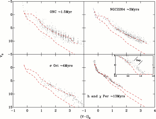
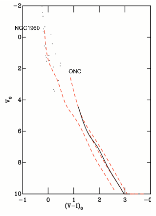
Figure 1 shows CMDs for members of a selection of young clusters and associations. The majority of the stars lie on the PMS, which is elevated in the diagram with respect to the main sequence (MS). For older groups the stars lie closer to the MS, and this decline in luminosity with time is an age indicator. If the isochronal models for PMS stars were good fits to the data we could simply use the best-fitting ages. However, in practice the data deviate systematically from the isochrone (e.g. [Bonatto (2004), Bonatto 2004]; [Pinsonneault et al. (2004), Pinsonneault et al., 2004]). Furthermore the derived ages can depend on which colour is fitted (e.g. [Naylor et al (2002), Naylor et al, 2002]). An obvious alternative is to abandon attempts to allocate absolute ages, but develop an age order (or ladder) based on the luminosity of the PMS. Simply plotting the data for different groups in the same diagram does not lead to useful results because the spread in each sequence is large. We therefore fit splines through each sequence, and place the splines in absolute-magnitude, intrinsic-colour space. The result of such a procedure is shown in Figure 2 (left), where we can see that NGC2264 is older than the ONC, but younger than NGC1960 and about the same age as $\sigma$ Ori.

Figure 1: The CMDs for a selection of young groups in absolute magnitude and intrinsic colour. In each case the lower red dotted line is the position of the MS, the upper an appropriate [Siess et al (2000), Siess et al (2000)] isochrone.

We used the above method in [Mayne et al (2007), Mayne et al (2007)] to obtain an age order for a set of well known clusters and associations, but realised that the limiting factor was the determination of the distance (with which the age is degenerate). So, in [Mayne & Naylor (2008), Mayne & Naylor (2008)] we measured the distances to these clusters and associations in a consistent way. As can be seen in Figure 1 the most massive stars are actually on the MS. We therefore fitted these stars to a MS model using $\tau^{2}$ fitting (see [Naylor & Jeffries (2006), Naylor & Jeffries, 2006] and Section 4) to derive distances. In Table 1 we present the resulting age ordering, including two more associations from more recent work. Although we give ages in Table 1, it is worth emphasising that strictly speaking we only derive an order. The ages represent an informed average of literature PMS ages for these groups.

Table 1: The Empirical Isochrone Age Ladder.

Age	Groups
1Myr	IC 5146
2Myr	ONC, NGC 6530
3Myr	$\lambda$ Ori, $\sigma$ Ori, NGC 2264
4-5Myr	IC 348, Cep OB3b1, NGC 2362
5-10Myr	$\gamma$ Vel2
10Myr	NGC 7160
13Myr	h and & $\chi$ Per
40Myr	NGC 2547

Notes: From [Mayne & Naylor (2008), Mayne & Naylor (2008)], except for: ¹Littlefair (in prep); ²[Jeffries et al. (2008), Jeffries et al (2008)]

3 Radiative-convective gap

An interesting feature of Figure 1 is the paucity of stars on the PMS isochrone immediately prior to the point where it joins the MS. The gap is clear and wide for the youngest groups, but by the age of h and $\chi$ Per has narrowed almost to the point of invisibility. The physical explanation for the gap lies in the change of structure between the fully convective interiors of PMS stars, and the partially radiative ones of MS stars. This drives a change in radius, which happens relatively quickly, leading to a rapid movement to bluer colours in the CMD, as stars move from the PMS to the MS. Hence in [Mayne et al (2007), Mayne et al (2007)] we named this the radiative convective gap.

Clearly this change in the size of the gap with age could be used an age indicator. It has two main advantages over PMS (contraction) ages. First, it uses brighter stars. Second, since one is measuring a distance, rather than position on colour-magnitude space, it is independent of errors in distance or extinction (assuming the latter is uniform). Before it can be used as an age indicator, though, it will need to be calibrated against ages derived from other techniques.

4 Nuclear (not quite turn-off) ages

Figure 2: Left: The empirical isochrone for NGC2264 (black curve), compared with other clusters and associations (the red dashed curves). The unmarked red dashed isochrone close to that for NGC2264 is $\sigma$ Ori. Right: Geneva-Bessell isochrones fitted to the NGC6530 data of [Walker (1957), Walker (1957)]. Each star has been dereddened using its position in a $U-B$/$B-V$ diagram. The fit in the left hand panel had the age fixed at 0.25Myr-old, yielding $Pr(\tau^{2})=0.03$. On the right the age was a free parameter, found to be 5.5Myr, with $Pr(\tau^{2})=0.67$.

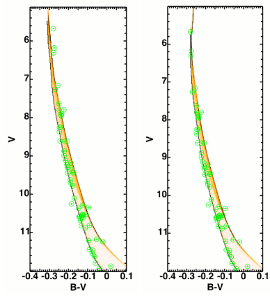
Before stars turn off the MS, they evolve redwards away from the zero-age MS, driven by their nuclear evolution. This means that in colour-magnitude space the MS, which normally has a positive gradient can, near its high-mass terminus, be vertical or even have a negative gradient (see Figure 2 (right)). Although the effect is subtle, if we can fit it, this should provide an age indicator. The best method for doing this is the $\tau^{2}$ method we described in [Naylor & Jeffries (2006), Naylor & Jeffries (2006)], since this allows for the effects of binarity, gives reliable uncertainties for the parameters, and provides a goodness-of-fit test. Unfortunately the technique as we described it will not work if the isochrone is vertical. Therefore we first outline the improvements which we have made to the method to allow us to address this problem (which will be described in more detail in Naylor in prep.), before moving on to our results.

4.1 Improvements to the $\tau^{2}$ technique

The technique relies on a finely sampled grid (such as the colour scales of Figure 2 (right)), which is a model created from of order a million simulated stars. We refer to this as $\rho(c,m)$ where $c$ and $m$ are the colour and magnitude co-ordinates respectively. For any given datapoint we calculate $\tau^{2}$ by multiplying this grid on a point-by-point basis with a function representing the datapoint and its uncertainties (typically a two-dimensional Gaussian). We represent this as $U_{i}(c-c_{i},m-m_{i})$, where $i$ is the index of a datapoint at co-ordinates $(c_{i},m_{i})$. If we now sum the resulting points, and repeat this over all datapoints we arrive at the definition of $\tau^{2}$

$$\tau^{2}=-2\sum_{i=1,N}{\rm ln}\int{U_{i}(c-c_{i},m-m_{i})\rho(c,m){\rm d}c\ {\rm d}m}.$$ (1)

The best-fitting model corresponds to the lowest value of $\tau^{2}$. For example, a simple fit in distance modulus can be viewed as moving the models up and down in Figure 2 (right) until the “cross correlation” between the datapoints and the model is maximised. In practice the simplest way to find the best fitting model is to calculate $\tau^{2}$ for a grid of models covering the range of parameters of interest.

There is a question as to how $\rho$ should be normalised. In [Naylor & Jeffries (2006), Naylor & Jeffries (2006)] we derived a normalisation such that Equation 1 reduced to that for $\chi^{2}$ for fitting a curve to data with uncertainties in one dimension. Unfortunately, when the isochrone is vertical, this results in an infinity in Equation 17 of that paper making it impractical for post-main-sequence fitting. Instead we now use a normalisation where the integral of $\rho$ between the faintest and brightest datapoints is one. Similarly we demand that the integral of $U$ is one over the entire CMD.

Having found a fit to the data, we must establish whether it is a good fit. We do this by calculating the probability that we would obtain our value of $\tau^{2}$ from observations, assuming the model was correct. This is $Pr(\tau^{2})$, which we showed how to calculate for no free parameters in [Naylor & Jeffries (2006), Naylor & Jeffries (2006)]. Our suggested correction to allow for free parameters, multiplying the values of $\tau^{2}$ by $(N-n)/N$ (where $N$ is the number of datapoints and $n$ the number of free parameters), is not invariant under changes in normalisation. A better approximation is to subtract the expectation value of $\tau^{2}$ before multiplying by $(N-n)/N$, and then add the expectation value on again.

Finally, to find the uncertainties in the parameters we have found a quicker method than that we presented in [Naylor & Jeffries (2006), Naylor & Jeffries (2006)]. Assuming the minimum value of $\tau^{2}$ has been found by a grid search, each datapoint in the grid has a probability $P$ associated with it (via the definition of $\tau^{2}$) of

$$P=e^{-{\tau^{2}}/2}.$$ (2)

By summing the probability below a given $\tau^{2}$, and dividing by the probability summed over the entire grid, one can obtain the probability that $\tau^{2}$ lies below a given value. This allows one to draw a confidence contour in the parameter space, in an identical fashion to that used in $\chi^{2}$ analysis.

4.2 Results

We have fitted UBV photometry for bright stars in NGC6530, NGC2264, $\sigma$ Ori, $\lambda$ Ori, NGC2362, Cep OB3b, NGC2547, IC2602 and stars in the vicinity of the Orion Nebula Cluster. For preference we have used data from the 1950s to 1970s of Walker, Johnson and collaborators, since this is a relatively homogeneous group of datasets, and we find our models fit them well. We have used the Geneva-Bessell models described in [Mayne & Naylor (2008), Mayne & Naylor (2008)]. We first use a $U-B$/$B-V$ diagram to determine the extinction. In some cases the extinction is uniform, and we determine its value using $\tau^{2}$ fitting. In other cases we find the extinction is non-uniform, and we find the extinctions on a star-by-star basis by comparison with the isochrone as described in [Mayne & Naylor (2008), Mayne & Naylor (2008)]. This is essentially an updated $Q$ method. We then perform a grid search in both age and distance to derive ages and associated uncertainties. Unsurprisingly our distances are all consistent with those in [Mayne & Naylor (2008), Mayne & Naylor (2008)], but for the groups less than 10Myr old, we find the ages are a factor 1.5-2.0 larger than those given in Table 1.

Before attaching any significance to this result, we questioned whether it could be due to either our fitting procedure or the models used. We have experimented with models without convective overshoot, which we find give poor fits to the data, and with the Padova models ([Girardi et al (2002), Girardi et al 2002]), which we find give similar answers to the Geneva-Bessell isochrones, though both models have yet to be tested exhaustively. We also find that our age for stars in the vicinity of the ONC (5Myr) is similar to that found using the same dataset by [Meynet et al (1993), Meynet et al (1993)]. For IC2602 [Mermilliod (1981), Mermilliod (1981)] obtains a nuclear age of 35Myr, which compares favourably with our estimate of about 40Myr. For NGC 2547 we obtain about 45Myr, compared with [Claria (1982), Claria (1982)] who obtains 57Myr. Since our ages are broadly consistent with other turn-off/nuclear ages, we can rule out some systematic effect from our models or fitting procedure. We are, therefore, forced to conclude that this is a genuine discrepancy between PMS ages and nuclear ages.

For the groups older than 10Myr it is harder to be definitive about any difference. The problem is we need both PMS photometry (to obtain an age on the same scale as Table 1) and good photo-electric photometry to obtain a nuclear age. We can carry out the test for NGC2547 for which we obtain 45Myr, compared with PMS and Lithium depletion ages of about 38Myr ([Naylor & Jeffries (2006), Naylor & Jeffries, 2006]) suggesting the discrepancy decreases with age. For IC2602 the situation is more ambiguous. The age we obtain (40Myr) is larger than the PMS age of 25Myr found by [Stauffer et al (1997), Stauffer et al (1997)], but is consistent with the finding of [Jeffries et al 2000, Jeffries et al (2000)] that IC2602 is a little older than NGC2547. Thus the question as to whether this discrepancy disappears for older clusters (and if so at what age) must await obtaining further PMS ages for older clusters.

4.3 Implications

It appears we have found a genuine difference between the PMS contraction and MS nuclear age scales. It is hard at this stage to decide which scale is correct, but as most modern work relies on the PMS age scale, it is interesting to examine the implications of the nuclear age scale being correct. It would help address two outstanding problems in the area. First, it is well known that that there appears to be a lack of clusters in the age range 5-30Myr ([Jeffries et al 2007, Jeffries et al, 2007]). Changing the ages in the way we suggest would fill that gap, especially if there is a return to the classical age scale for clusters older than 30Myr. Second there is a problem in the disc-clearing timescale measured from IR observations of young stars (of order 3Myr, e.g. [Briceño et al (2007), Briceño et al, 2007]) and the time required to form a planet by classical core accretion (perhaps 9Myr; [Pollack et al (1996), Pollack et al, 1996]). Whilst there are active attempts to solve this problem by reducing the theoretical timescale (e.g. [Dodson-Robinson et al (2008), Dodson-Robinson et al, 2008] and references therein), our work supports a different solution - increasing the observed timescale by a factor two.

Figure 3: PMS vs nuclear ages for young clusters and associations. The datapoints would lie on the line if they were equal. The error bars show the uncertainties derived from the $\tau^{2}$ fitting.

References

- [Bonatto (2004)] Bonatto, C., Bica, E. & Girardi, L. 2004, A&A 415, 571
- [Briceño et al (2007)] Briceño, C., Preibisch, T., Sherry, W. H., Mamajek, E. A., Mathieu, R. D., Walter, F. M. & Zinnecker, H., in proceedings of Protostars and Planets V p345
- [Claria (1982)] Claria, J. J., 1982, A&AS 47, 323
- [Dodson-Robinson et al (2008)] Dodson-Robinson, S. E., Bodenheimer, P., Laughlin, G., Willacy, K., Turner, N. J. & Beichman, C. A., 2008, 2008arXiv0810.0288D
- [Girardi et al (2002)] Girardi, L., Bertelli, G., Bressan, A., Chiosi, C., Groenewegen, M. A. T., Marigo, P., Salasnich, B., & Weiss, A. 2002, A&A 391, 195
- [Jeffries et al 2000] Jeffries, R. D., Totten, E. J. & James, D. J., 2000, MNRAS 316, 950
- [Jeffries et al 2007] Jeffries, R. D., Oliveira, J. M., Naylor, T., Mayne, N. J. & Littlefair, S. P. 2007, MNRAS 376, 580
- [Jeffries et al. (2008)] Jeffries, R.D., Naylor, T., Walter, F.M., Pozzo, M.P., & Devey, C. R., 2008, MNRAS, accepted, arXiv:0810.5320
- [Mayne & Naylor (2008)] Mayne, N.J., & Naylor, T., 2008, MNRAS 386, 261
- [Mayne et al (2007)] Mayne, N. J.,Naylor, T., Littlefair, S. P., Saunders, E. S. & Jeffries, R. D., 2007, MNRAS 375, 1220
- [Mermilliod (1981)] Mermilliod, J. C., 1981, A&A 97, 235
- [Meynet et al (1993)] Meynet, G., Mermilliod, J.-C., & Maeder, A., 1993, A&AS 98, 477
- [Naylor et al (2002)] Naylor, T., Totten, E. J., Jeffries, R. D., Pozzo, M., Devey, C. R. & Thompson, S. A. 2002, MNRAS 335, 291
- [Naylor & Jeffries (2006)] Naylor, T., & Jeffries, R.D. 2006, MNRAS 373, 1251
- [Pinsonneault et al. (2004)] Pinsonneault, M. H., Terndrup, D. M., Hanson, R. B., Stauffer, J. R. 2004, ApJ 600, 946
- [Pollack et al (1996)] Pollack, J. B., Hubickyj, O., Bodenheimer, P., Lissauer, J. J., Podolak, M. & Greenzweig, Y., Icarus 124, 62
- [Siess et al (2000)] Siess, L., Dufour, E. & Forestini, M. 2000, ApJ 358, 593
- [Stauffer et al (1997)] Stauffer, J. R., Hartmann, L. W., Prosser, C. F., Randich, S., Balachandran, S., Patten, B. M., Simon, T. & Giampapa, M., 1997, ApJ 479, 776
- [Walker (1957)] Walker, M. F. 1957, ApJ 125, 636