Lower Bounds for BMRM and Faster Rates for Training SVMs

Abstract

Regularized risk minimization with the binary hinge loss and its variants lies at the heart of many machine learning problems. Bundle methods for regularized risk minimization (BMRM) and the closely related SVMStruct are considered the best general purpose solvers to tackle this problem. It was recently shown that BMRM requires $O(1/\varepsilon)$ iterations to converge to an $\varepsilon$ accurate solution. In the first part of the paper we use the Hadamard matrix to construct a regularized risk minimization problem and show that these rates cannot be improved. We then show how one can exploit the structure of the objective function to devise an algorithm for the binary hinge loss which converges to an $\varepsilon$ accurate solution in $O(1/\sqrt{\varepsilon})$ iterations.

1 Introduction

Let $\mathbf{x}_{i}\in\mathcal{X}\subseteq\mathbb{R}^{d}$ denote samples and $\mathbf{y}_{i}\in\mathcal{Y}$ be the corresponding labels. Given a training set of $n$ sample label pairs $\left\{(\mathbf{x}_{i},\mathbf{y}_{i})\right\}_{i=1}^{n}$, drawn i.i.d. from a joint probability distribution on $\mathcal{X}\times\mathcal{Y}$, many machine learning algorithms solve the following regularized risk minimization problem:

$$\min_{\mathbf{w}}J(\mathbf{w}):=\lambda\Omega(\mathbf{w})+R_{{\mathrm{emp}}}(\mathbf{w}),\text{ where }R_{{\mathrm{emp}}}(\mathbf{w}):=\frac{1}{n}\sum_{i=1}^{n}l(\mathbf{x}_{i},\mathbf{y}_{i};\mathbf{w}).\vspace{-1em}$$ (1)

Here $l(\mathbf{x}_{i},\mathbf{y}_{i};\mathbf{w})$ denotes the loss on instance $(\mathbf{x}_{i},\mathbf{y}_{i})$ using the current model $\mathbf{w}$ and $R_{{\mathrm{emp}}}(\mathbf{w})$, the empirical risk, is the average loss on the training set. The regularizer $\Omega(\mathbf{w})$ acts as a penalty on the complexity of the classifier and prevents overfitting. Usually the loss is convex in $\mathbf{w}$ but can be nonsmooth while the regularizer is usually a smooth strongly convex function. Binary Support Vector Machines (SVMs) are a prototypical example of such regularized risk minimization problems where $\mathcal{Y}=\{1,-1\}$ and the loss considered is the binary hinge loss:

$$l(\mathbf{x}_{i},y_{i};\mathbf{w})=\left[1-y_{i}\left\langle\mathbf{w},\mathbf{x}_{i}\right\rangle\right]_{+},\text{ with }\left[\cdot\right]_{+}:=\max(0,\cdot).$$ (2)

Recently, a number of solvers have been proposed for the regularized risk minimization problem. The first and perhaps the best known solver is SVMStruct [1], which was shown to converge in $O(1/\varepsilon^{2})$ iterations to an $\varepsilon$ accurate solution. The convergence analysis of SVMStruct was improved to $O(1/\varepsilon)$ iterations by [2]. In fact, [2] showed that their convergence analysis holds for a more general solver than SVMStruct namely BMRM (Bundle method for regularized risk minimization).

At every iteration BMRM replaces $R_{{\mathrm{emp}}}$ by a piecewise linear lower bound $R^{\mathrm{cp}}_{t}$ and optimizes

$$\min_{\mathbf{w}}J_{t}(\mathbf{w}):=\lambda\Omega(\mathbf{w})+R^{\mathrm{cp}}_{t}(\mathbf{w}),\text{where }R^{\mathrm{cp}}_{t}(\mathbf{w}):=\max_{1\leq i\leq t}\left\langle\mathbf{w},\mathbf{a}_{i}\right\rangle+b_{i},$$ (3)

to obtain the next iterate $\mathbf{w}_{t}$. Here $\mathbf{a}_{i}\in\partial R_{{\mathrm{emp}}}(\mathbf{w}_{i-1})$ denotes an arbitrary subgradient of $R_{{\mathrm{emp}}}$ at $\mathbf{w}_{i-1}$ (see Section 2) and $b_{i}=R_{{\mathrm{emp}}}(\mathbf{w}_{i-1})-\left\langle\mathbf{w}_{i-1},\mathbf{a}_{i}\right\rangle$. The piecewise linear lower bound is successively tightened until the gap

$$\varepsilon_{t}:=\min_{0\leq t^{\prime}\leq t}J(\mathbf{w}_{t^{\prime}})-J_{t}(\mathbf{w}_{t}),$$ (4)

falls below a predefined tolerance $\varepsilon$.

Even though BMRM solves an expensive optimization problem at every iteration, the convergence analysis only uses a simple one-dimensional line search to bound the decrease in $\varepsilon_{t}$. Furthermore, the empirical convergence behavior of BMRM is much better than the theoretically predicted rates on a number of real life problems. It was therefore conjectured that the rates of convergence of BMRM could be improved. In this paper we answer this question in the negative by explicitly constructing a regularized risk minimization problem for which BMRM takes at least $O(1/\varepsilon)$ iterations.

One possible way to circumvent the $O(1/\varepsilon)$ lower bound is to solve the problem in the dual. Using a very old result of Nesterov [3] we obtain an algorithm for SVMs which only requires $O(1/\sqrt{\varepsilon})$ iterations to converge to an $\varepsilon$ accurate solution; each iteration of the algorithm requires $O(nd)$ work. Although we primarily focus on the regularized risk minimization with the binary hinge loss, our algorithm can also be used whenever the empirical risk is piecewise linear and contains a small number of pieces. Examples of this include multiclass, multi-label, and ordinal regression hinge loss and other related losses.

2 Preliminaries

In this paper, lower bold case letters (e.g., $\mathbf{w}$, $\bm{\mu}$) denote vectors, $w_{i}$ denotes the $i$-th component of $\mathbf{w}$ and $\Delta_{k}$ refers to the $k$ dimensional simplex. Unless specified otherwise, $\left\|\cdot\right\|$ refers to the Euclidean norm $\|\mathbf{w}\|:=\left(\sum_{i=1}^{n}w_{i}^{2}\right)^{\frac{1}{2}}$. $\overline{\mathbb{R}}:=\mathbb{R}\cup\{\infty\}$, and $[t]:=\{1,\ldots,t\}$. The $\mathrm{dom}$ of a convex function $F$ is defined by $\mathrm{dom}\ F:=\left\{\mathbf{w}:F(\mathbf{w})<\infty\right\}$. The following three notions will be used extensively:

Definition 1

A convex function $F:\mathbb{R}^{n}\to\overline{\mathbb{R}}$ is strongly convex (s.c.) wrt norm $\|\cdot\|$ if there exists a constant $\sigma>0$ such that $F-\frac{\sigma}{2}\|\cdot\|^{2}$ is convex. $\sigma$ is called the modulus of strong convexity of $F$, and for brevity we will call $F$ $\sigma$-strongly convex or $\sigma$-s.c..

Definition 2

A function $F$ is said to have Lipschitz continuous gradient (l.c.g) if there exists a constant $L$ such that

$$\|\nabla F(\mathbf{w})-\nabla F(\mathbf{w}^{\prime})\|\leq L\|\mathbf{w}-\mathbf{w}^{\prime}\|\qquad\forall\ \mathbf{w}\text{ and }\mathbf{w}^{\prime}.$$ (5)

For brevity, we will call $F$ $L$-l.c.g..

Definition 3

The Fenchel dual of a function $F:E_{1}\to E_{2}$, is a function $F^{\star}:E_{2}^{\star}\to E_{1}^{\star}$ given by

$$F^{\star}(\mathbf{w}^{\star})=\sup_{\mathbf{w}\in E_{1}}\left\{\left\langle\mathbf{w},\mathbf{w}^{\star}\right\rangle-F(\mathbf{w})\right\}$$ (6)

The following theorem specifies the relationship between strong convexity of a primal function and Lipschitz continuity of the gradient of its Fenchel dual.

Theorem 4 ([4, Theorem 4.2.1 and 4.2.2])

 

1. If $F:\mathbb{R}^{n}\to\overline{\mathbb{R}}$ is $\sigma$-strongly convex, then $\mathrm{dom}\ F^{\star}=\mathbb{R}^{n}$ and ${\nabla}F^{\star}$ is $\frac{1}{\sigma}$-l.c.g.

2. If $F:\mathbb{R}^{n}\to\mathbb{R}$ is convex and $L$-l.c.g, then $F^{\star}$ is $\frac{1}{L}$-strongly convex.

Subgradients generalize the concept of gradients to nonsmooth functions. For $\mathbf{w}\in\mathrm{dom}\ F$, $\bm{\mu}$ is called a subgradient of $F$ at $\mathbf{w}$ if

$$F(\mathbf{w}^{\prime})\geq F(\mathbf{w})+\left\langle\mathbf{w}^{\prime}-\mathbf{w},\bm{\mu}\right\rangle\quad\forall\mathbf{w}^{\prime}.$$ (7)

The set of all subgradients at $\mathbf{w}$ is called the subdifferential, denoted by $\partial F(\mathbf{w})$. If $F$ is convex, then $\partial F(\mathbf{w})\neq\emptyset$ for all $\mathbf{w}\in\mathrm{dom}\ F$, and is a singleton if, and only if, $F$ is differentiable [4].

Any piecewise linear convex function $F(\mathbf{w})$ with $t$ linear pieces can be written as

$$F(\mathbf{w})=\max_{i\in[t]}\{\left\langle\mathbf{a}_{i},\mathbf{w}\right\rangle+b_{i}\},$$ (8)

for some $\mathbf{a}_{i}$ and $b_{i}$. If the empirical risk $R_{{\mathrm{emp}}}$ is a piecewise linear function then the convex optimization problem in (1) can be expressed as

$$\min_{\mathbf{w}}J(\mathbf{w}):=\min_{\mathbf{w}}\max_{i\in[t]}\{\left\langle\mathbf{a}_{i},\mathbf{w}\right\rangle+b_{i}\}+\lambda\Omega(\mathbf{w}).$$ (9)

Let $\mathbf{A}=[\mathbf{a}_{1}\ldots\mathbf{a}_{t}]$, then the adjoint form of $J(\mathbf{w})$ can be written as

$$D(\bm{\alpha}):=-\lambda\Omega^{\star}(-\lambda^{-1}\mathbf{A}\bm{\alpha})+\left\langle\bm{\alpha},b\right\rangle\text{ with }\bm{\alpha}\in\Delta_{t}$$ (10)

where the primal and the adjoint optimum are related by

$$\mathbf{w}^{*}=\partial\Omega^{\star}(-\lambda^{-1}\mathbf{A}\bm{\alpha}^{*})$$ (11)

In fact, using concepts of strong duality (see e.g.Theorem 2 of [5]), it can be shown that

$$\inf_{\mathbf{w}\in\mathbb{R}^{d}}\left\{\max_{i\in[n]}\left\langle\mathbf{a}_{i},\mathbf{w}\right\rangle+b_{i}+\lambda\Omega(\mathbf{w})\right\}=\sup_{\bm{\alpha}\in\Delta_{t}}\left\{-\lambda\Omega^{\star}(-\lambda^{-1}\mathbf{A}\bm{\alpha})+\left\langle\bm{\alpha},\mathbf{b}\right\rangle\right\}$$ (12)

3 Lower Bounds

The following result was shown by [2]:

Theorem 5 (Theorem 4 of [2])

Assume that $J(\mathbf{w})\geq 0$ for all $\mathbf{w}$, and that $\left\|\partial_{\mathbf{w}}R_{{\mathrm{emp}}}(\mathbf{w})\right\|\leq G$ for all $\mathbf{w}\in W$, where $W$ is some domain of interest containing all $\mathbf{w}_{t^{\prime}}$ for $t^{\prime}\leq t$. Also assume that $\Omega^{*}$ has bounded curvature, i.e. let $\left\|\partial^{2}_{\mu}\Omega^{*}(\bm{\mu})\right\|\leq H^{*}$ for all $\bm{\mu}\in\left\{-\lambda^{-1}A\bm{\alpha}\text{ where }\bm{\alpha}\in\Delta_{t}\right\}$. Then, for any $\varepsilon<4G^{2}H^{*}/\lambda$ we have $\varepsilon_{t}<\varepsilon$ after at most

$$\log_{2}\frac{\lambda J(\mathbf{0})}{G^{2}H^{*}}+\frac{8G^{2}H^{*}}{\lambda\varepsilon}-4$$ (13)

steps.

Although the above theorem proves an upper bound of $O(1/\varepsilon)$ on the number of iterations, the tightness of this bound has been an open question. We now demonstrate a function which satisfies all the conditions of the above theorem, and yet takes $\Omega(1/\varepsilon)$ iterations to converge.

To construct our lower bounds we make use of the Hadamard matrix. An $n\times n$ Hadamard matrix is an orthogonal matrix with $\{\pm 1\}$ elements which is recursively defined for $d=2^{k}$ (for some $k$):

$\mathbf{H}_{1}=\left(+1\right)$

$\mathbf{H}_{2}=\left(\begin{array}[]{cc}+1&+1\\ +1&-1\end{array}\right)$

$\mathbf{H}_{2d}=\left(\begin{array}[]{cc}\mathbf{H}_{d}&\;\;\mathbf{H}_{d}\\ \mathbf{H}_{d}&-\mathbf{H}_{d}\end{array}\right)$

Note that all rows of the Hadamard matrix $\mathbf{H}_{d}$ are orthogonal and have Euclidean norm $\sqrt{d}$. Consider the following $d\times d$ orthonormal matrix

$$\mathbf{A}:=\frac{1}{\sqrt{d}}\left(\begin{array}[]{cc}\mathbf{H}_{d/2}&-\mathbf{H}_{d/2}\\ -\mathbf{H}_{d/2}&\mathbf{H}_{d/2}\end{array}\right),$$

whose columns $\mathbf{a}_{i}$ are orthogonal and have Euclidean norm $1$, which is used to define the following piecewise quadratic function:

$$J(\mathbf{w}) =\underbrace{\max_{i\in[d]}\left\langle\mathbf{a}_{i},\mathbf{w}\right\rangle}_{R_{{\mathrm{emp}}}}+\underbrace{\frac{\lambda}{2}\|\mathbf{w}\|^{2}}_{\lambda\Omega(\mathbf{w})}.$$ (14)

Theorem 6

The function $J(\mathbf{w})$ defined in (14) satisfies all the conditions of Theorem 5. For any $t<\frac{d}{2}$ we have $\varepsilon_{t}\geq\frac{1}{2\lambda t}$.

Proof  By construction of $\mathbf{A}$, we have $\max_{i\in[d]}\left\langle\mathbf{a}_{i},\mathbf{w}\right\rangle\geq 0$. Furthermore, $\frac{\lambda}{2}\|\mathbf{w}\|^{2}\geq 0$. Together this implies that $J(\mathbf{w})\geq 0$. Furthermore, $\partial_{\mathbf{w}}R_{{\mathrm{emp}}}(\mathbf{w})$ are the columns of $\mathbf{A}$, which implies that $\left\|\partial_{\mathbf{w}}R_{{\mathrm{emp}}}(\mathbf{w})\right\|\leq 1$. Since we set $\Omega(\cdot)=\frac{1}{2}\|\cdot\|^{2}$ it follows that $\Omega^{*}(\cdot)=\frac{1}{2}\|\cdot\|^{2}$. Therefore $\left\|\partial^{2}_{\mu}\Omega^{*}(\cdot)\right\|=\frac{1}{2}$. Hence, (14) satisfies all the conditions of Theorem 5.

Let $\mathbf{w}_{0},\mathbf{w}_{1}\ldots\mathbf{w}_{t}$ denote the solution produced by BMRM after $t$ iterations, and let $\mathbf{a}_{i_{0}},\mathbf{a}_{i_{1}}\ldots\mathbf{a}_{i_{t}}$ denote the corresponding subgradients. Then

$$J_{t}(\mathbf{w}) =\max_{j\in[t]}\left\langle\mathbf{a}_{i_{j}},\mathbf{w}\right\rangle+\frac{\lambda}{2}\|\mathbf{w}\|^{2}\text{ with }\mathbf{w}_{t}=\mathop{\mathrm{argmin}}_{\mathbf{w}\in\mathbb{R}^{d}}J_{t}(\mathbf{w}).$$ (15)

If we define $\mathbf{A}_{t}=[\mathbf{a}_{i_{j}}]$ with $j\in[t]$ then

$$J_{t}(\mathbf{w}_{t}) =\min_{\mathbf{w}\in\mathbb{R}^{d}}\max_{j\in[t]}\left\langle\mathbf{a}_{i_{j}},\mathbf{w}\right\rangle+\frac{\lambda}{2}\|\mathbf{w}\|^{2}=\min_{\mathbf{w}\in\mathbb{R}^{d}}\max_{\bm{\alpha}\in\Delta^{t}}\mathbf{w}^{\top}\mathbf{A}_{t}\bm{\alpha}+\frac{\lambda}{2}\|\mathbf{w}\|^{2}$$

$$=\max_{\bm{\alpha}\in\Delta^{t}}\min_{\mathbf{w}\in\mathbb{R}^{d}}\mathbf{w}^{\top}\mathbf{A}_{t}\bm{\alpha}+\frac{\lambda}{2}\|\mathbf{w}\|^{2}\hskip 8.53581pt\text{( See Appendix \ref{sec:MinimaxTheoremConvex} for details)}$$ (16)

$$=\max_{\bm{\alpha}\in\Delta^{t}}-\frac{1}{2\lambda}\bm{\alpha}^{\top}\mathbf{A}_{t}^{\top}\mathbf{A}_{t}\bm{\alpha}=-\min_{\bm{\alpha}\in\Delta^{t}}\frac{1}{2\lambda}\bm{\alpha}^{\top}\mathbf{A}_{t}^{\top}\mathbf{A}_{t}\bm{\alpha}.$$

Since the columns of $\mathbf{A}$ are orthonormal, it follows that $\mathbf{A}_{t}^{\top}\mathbf{A}=\mathbf{I}_{t}$ where $\mathbf{I}_{t}$ is the $t$ $\times$ $t$ dimensional identity matrix. Thus

$$J_{t}(\mathbf{w}_{t})=-\frac{1}{2\lambda}\min_{\alpha\in\Delta^{t}}\|\bm{\alpha}\|^{2}=-\frac{1}{2\lambda}\frac{1}{t}$$

Combining this with $J(\mathbf{w}_{t^{\prime}})\geq 0$ for $t^{\prime}\in[t]$ and recalling the definition of $\varepsilon_{t}$ from (4) completes the proof.  
In fact, $\varepsilon_{t}$ is a proxy for the primal gap

$$\delta_{t}=\min_{t^{\prime}\in[t]}J(\mathbf{w}_{t^{\prime}})-J(\mathbf{w}^{*}).$$

Since $J(\mathbf{w}^{*})$ is unknown, it is replaced by $J_{t}(\mathbf{w}_{t})$ to obtain $\varepsilon_{t}$. Since $J(\mathbf{w}^{*})\geq J_{t}(\mathbf{w}_{t})$, it follows that $\varepsilon_{t}\geq\delta_{t}$ [5]. We now show that Theorem 6 holds even if we replace $\varepsilon_{t}$ by $\delta_{t}$.

Theorem 7

Under the same assumptions as Theorem 6, for any $t<\frac{d}{2}$ we have $\delta_{t}\geq\frac{1}{2\lambda t}$.

Proof  Note that $J_{t}(\mathbf{w})$ is minimized by setting $\alpha=\frac{1}{t}\mathbf{e}$, where $\mathbf{e}$ denotes the $t$ dimensional vector of ones. Recalling that $\Omega^{*}(\cdot)=\frac{1}{2}\|\cdot\|^{2}$ and using (11) one can write $\mathbf{w}_{t}=-\frac{1}{t\lambda}\mathbf{A}_{t}\mathbf{e}$. Since the columns of $\mathbf{A}$ are orthonormal, it follows that $\left\langle\mathbf{a}_{i},\mathbf{w}_{t}\right\rangle$ is $-\frac{1}{t\lambda}$ if $\mathbf{a}_{i}$ is a column of $\mathbf{A}_{t}$ and 0 otherwise. Therefore, $\max_{i\in[d]}\left\langle\mathbf{a}_{i},\mathbf{w}_{t}\right\rangle=0$. On the other hand, by noting that $\mathbf{A}_{t}^{\top}\mathbf{A}=\mathbf{I}_{t}$ we obtain $\frac{\lambda}{2}||\mathbf{w}_{t}||^{2}=\frac{1}{2t\lambda}$. Plugging into (14) yields $J(\mathbf{w}_{t})=\frac{1}{2t\lambda}$ and hence $\min_{t^{\prime}\in[t]}J(\mathbf{w}_{t^{\prime}})=\frac{1}{2t\lambda}$. It remains to note that $J(\mathbf{w})\geq 0$, while $J(\mathbf{0})=0$. Therefore $J(\mathbf{w}^{*})=J(\mathbf{0})=0$.  

4 A new algorithm with convergence rates $O(1/\sqrt{\varepsilon})$

We now turn our attention to the regularized risk minimization with the binary hinge loss, and propose a new algorithm. Our algorithm is based on [3] and [6] which proposed a non-trivial scheme of minimizing an $L$-l.c.g function to $\varepsilon$-precision in $O(1/\sqrt{\varepsilon})$ iterations. Our contributions are two fold. First, we show that the dual of the regularized risk minimization problem is indeed a $L$-l.c.g function. Second, we introduce an $O(n)$ time algorithm for projecting onto an $n$-dimensional simplex or in general an $n$-dimensional box with a single linear equality constraint, thus improving upon the $O(n\log n)$ deterministic algorithm of [7] (which also gives a randomized algorithm having expected complexity $O(n)$). This projection is repeatedly invoked as a subroutine by Nesterov’s algorithm when specialized to our problem.

Consider the problem of minimizing a function $J(\mathbf{w})$ with the following structure over a closed convex set $Q_{1}$:

$$J(\mathbf{w})=f(\mathbf{w})+g^{\star}(\mathbf{A}\mathbf{w}).$$ (17)

Here $f$ is strongly convex on $Q_{1}$, $\mathbf{A}$ is a linear operator which maps $Q_{1}$ to another closed convex set $Q_{2}$, and $g$ is convex and l.c.g on $Q_{2}$. [6] works with the adjoint form of $J$:

$$D(\bm{\alpha})=-g(\bm{\alpha})-f^{\star}(-\mathbf{A}^{\top}\bm{\alpha}),$$ (18)

which is l.c.g according to Theorem 4. Under some mild constraint qualifications which we omit for the sake of brevity (see e.g. Theorem 3.3.5 of [8]) we have

$$J(\mathbf{w})\geq D(\bm{\alpha})\text{ and }\inf_{\mathbf{w}\in Q_{1}}J(\mathbf{w})=\sup_{\bm{\alpha}\in Q_{2}}D(\bm{\alpha}).$$ (19)

By using the algorithm in [3] to maximize $D(\bm{\alpha})$ one can obtain an algorithm which converges to an $\varepsilon$ accurate solution of $J(\mathbf{w})$ in $O(1/\sqrt{\varepsilon})$ iterations.

The regularized risk minimization with the binary hinge loss can be identified with (17) by setting

$$J(\mathbf{w})=\underbrace{\frac{\lambda}{2}\left\|\mathbf{w}\right\|^{2}}_{f(\mathbf{w})}+\underbrace{\min_{b\in\mathbb{R}}\frac{1}{n}\sum_{i=1}^{n}\left[1-y_{i}(\left\langle\mathbf{x}_{i},\mathbf{w}\right\rangle+b)\right]_{+}}_{g^{\star}(\mathbf{A}\mathbf{w})}$$ (20)

The latter, $g^{\star}$, is the dual of $g(\bm{\alpha})=-\sum_{i}\alpha_{i}$ (see Appendix C). Here $Q_{1}=\mathbb{R}^{d}$. Let $\mathbf{A}:=-\mathbf{Y}\mathbf{X}^{\top}$ where $\mathbf{Y}:=\mathop{\mathrm{diag}}(y_{1},\ldots,y_{n})$, $\mathbf{X}:=[\mathbf{x}_{1},\ldots,\mathbf{x}_{n}]$. Then the adjoint can be written as :

$$D(\bm{\alpha}) :=-g(\bm{\alpha})-f^{\star}(-\mathbf{A}^{\top}\bm{\alpha})=\sum_{i}\alpha_{i}-\frac{1}{2\lambda}\bm{\alpha}^{\top}\mathbf{Y}\mathbf{X}^{\top}\mathbf{X}\mathbf{Y}\bm{\alpha}\qquad\text{ with }$$ (21)

$$Q_{2} =\left\{\bm{\alpha}\in[0,n^{-1}]^{n}:\sum_{i}y_{i}\alpha_{i}=0\right\}.$$ (22)

In fact, this is the well known SVM dual objective function with the bias incorporated.

Now we present the algorithm of [6] in Algorithm 1. Since it optimizes the primal $J(\mathbf{w})$ and the adjoint $D(\bm{\alpha})$ simultaneously, we call it Pragam (PRimal-Adjoint GAp Minimization). It requires a $\sigma_{2}$-strongly convex prox-function on $Q_{2}$: $d_{2}(\bm{\alpha})=\frac{\sigma_{2}}{2}\|\bm{\alpha}\|^{2}$, and sets $D_{2}=\max_{\bm{\alpha}\in Q_{2}}d_{2}(\bm{\alpha})$. Let the Lipschitz constant of $\nabla D(\bm{\alpha})$ be $L$. Algorithm 1 is based on two mappings $\bm{\alpha}_{\mu}(\mathbf{w}):Q_{1}\mapsto Q_{2}$ and $\mathbf{w}(\bm{\alpha}):Q_{2}\mapsto Q_{1}$, together with an auxiliary mapping $v:Q_{2}\mapsto Q_{2}$. They are defined by

$$\bm{\alpha}_{\mu}(\mathbf{w}) :=\mathop{\mathrm{argmin}}_{\bm{\alpha}\in Q_{2}}\mu d_{2}(\bm{\alpha})-\left\langle\mathbf{A}\mathbf{w},\bm{\alpha}\right\rangle+g(\bm{\alpha})=\mathop{\mathrm{argmin}}_{\bm{\alpha}\in Q_{2}}\frac{\mu}{2}\left\|\bm{\alpha}\right\|^{2}+\mathbf{w}^{\top}\mathbf{X}\mathbf{Y}\bm{\alpha}-\sum_{i}\alpha_{i},$$ (23)

$$\mathbf{w}(\bm{\alpha}) :=\mathop{\mathrm{argmin}}_{\mathbf{w}\in Q_{1}}\left\langle\mathbf{A}\mathbf{w},\bm{\alpha}\right\rangle+f(\mathbf{w})=\mathop{\mathrm{argmin}}_{\mathbf{w}\in\mathbb{R}^{d}}-\mathbf{w}^{\top}\mathbf{X}\mathbf{Y}\bm{\alpha}+\frac{\lambda}{2}\left\|\mathbf{w}\right\|^{2}=\frac{1}{\lambda}\mathbf{X}\mathbf{Y}\bm{\alpha},$$ (24)

$$v(\bm{\alpha}) :=\mathop{\mathrm{argmin}}_{\bm{\alpha}^{\prime}\in Q_{2}}\frac{L}{2}\left\|\bm{\alpha}^{\prime}-\bm{\alpha}\right\|^{2}-\left\langle{\nabla}D(\bm{\alpha}),\bm{\alpha}^{\prime}-\bm{\alpha}\right\rangle.$$ (25)

Equations (23) and (25) are examples of a box constrained QP with a single equality constraint. In the appendix, we provide a linear time algorithm to find the minimizer of such a QP. The overall complexity of each iteration is thus $O(nd)$ due to the gradient calculation in (25) and the matrix multiplication in (24).

0:  $L$ as a conservative estimate of (i.e., no less than) the Lipschitz constant of ${\nabla}D(\bm{\alpha})$.

0:  Two sequences $\mathbf{w}_{k}$ and $\bm{\alpha}_{k}$ which reduce the duality gap at $O(1/k^{2})$ rate.

1:  Initialize: Randomly pick $\bm{\alpha}_{-1}$ in $Q_{2}$. Let $\mu_{0}=2L$, $\bm{\alpha}_{0}\leftarrow v(\bm{\alpha}_{-1})$, $\mathbf{w}_{0}\leftarrow\mathbf{w}(\bm{\alpha}_{-1})$.

2:  for $k=0,1,2,\ldots$ do

3:     Let $\tau_{k}=\frac{2}{k+3}$, $\bm{\beta}_{k}\leftarrow(1-\tau_{k})\bm{\alpha}_{k}+\tau_{k}\bm{\alpha}_{\mu_{k}}(\mathbf{w}_{k})$.

4:     Set $\mathbf{w}_{k+1}\leftarrow(1-\tau_{k})\mathbf{w}_{k}+\tau_{k}\mathbf{w}(\bm{\beta}_{k})$, $\bm{\alpha}_{k+1}\leftarrow v(\bm{\beta}_{k})$, $\mu_{k+1}\leftarrow(1-\tau_{k})\mu_{k}$.

5:  end for

Algorithm 1 Pragam: an $O(1/k^{2})$ rate primal-adjoint solver.

4.1 Convergence Rates

According to [6], on running Algorithm Pragam for $k$ iterations, the $\bm{\alpha}_{k}$ and $\mathbf{w}_{k}$ satisfy:

$$J(\mathbf{w}_{k})-D(\bm{\alpha}_{k})\leq\frac{4LD_{2}}{(k+1)(k+2)\sigma_{2}}.$$ (26)

For SVMs, $L=\frac{1}{\lambda}\left\|\mathbf{A}\right\|_{1,2}^{2}$ where $\left\|\mathbf{A}\right\|_{1,2}=\max\left\{\left\langle\mathbf{A}\mathbf{w},\bm{\alpha}\right\rangle:\left\|\bm{\alpha}\right\|=1,\left\|\mathbf{w}\right\|=1\right\}$, $\sigma_{2}=1$, $D_{2}=\frac{1}{2n}$. Assuming $\left\|\mathbf{x}_{i}\right\|\leq R$,

$$\left|\left\langle\mathbf{A}\mathbf{w},\bm{\alpha}\right\rangle\right|^{2} \leq\left\|\bm{\alpha}\right\|^{2}\left\|\mathbf{Y}\mathbf{X}^{\top}\mathbf{w}\right\|^{2}=\left\|\mathbf{X}^{\top}\mathbf{w}\right\|^{2}=\sum_{i}(\mathbf{x}_{i}^{\top}\mathbf{w})^{2}\leq\sum_{i}\left\|\mathbf{w}\right\|^{2}\left\|\mathbf{x}_{i}\right\|^{2}\leq nR^{2}.$$

Thus by (26), we conclude

$$J(\mathbf{w}_{k})-D(\bm{\alpha}_{k})\leq\frac{4LD_{2}}{(k+1)(k+2)\sigma_{2}}\leq\frac{2R^{2}}{\lambda(k+1)(k+2)}<\varepsilon,\qquad\text{ which gives }k>\left(\frac{R}{\sqrt{\lambda\varepsilon}}\right).$$

It should be noted that our algorithm has a better dependence on $\lambda$ compared to other state-of-the-art SVM solvers like Pegasos [9], SVM-Perf [10], and BMRM [5] which have a factor of $\frac{1}{\lambda}$ in their convergence rates. Our rate of convergence is also data dependent, showing how the correlation of the dataset $\mathbf{Y}\mathbf{X}=(y_{1}\mathbf{x}_{1},\ldots,y_{n}\mathbf{x}_{n})$ affects the rate via the Lipschitz constant $L$, which is equal to the square of the maximum singular value of $\mathbf{Y}\mathbf{X}$ (or the maximum eigenvalue of $\mathbf{Y}\mathbf{X}\mathbf{X}^{\top}\mathbf{Y}$). On one extreme, if $\mathbf{x}_{i}$ is the $i$-th dimensional unit vector then $L=1$, while $L=n$ if all $y_{i}\mathbf{x}_{i}$ are identical.

4.2 Structured Data

It is noteworthy that applying Pragam to structured data is straightforward. Due to space constraints, we present the details in Appendix E. A key interesting problem there is how to project onto a probability simplex such that the image decomposes according to a graphical model.

5 Experimental Results

In this section, we compare the empirical performance of our Pragam with state-of-the-art binary linear SVM solvers, including liblinear [11], pegasos [9], and BMRM [5].

Datasets

Table 1 lists the statistics of the dataset. adult9, astro-ph, news20, real-sim, reuters-c11, reuters-ccat are from the same source as in [11]. aut-avn classifies documents on auto and aviation (http://www.cs.umass.edu/$\sim$mccallum/data/sraa.tar.gz). covertype is from UCI repository. We did not normalize the feature vectors and no bias was used.

dataset	$n$	$d$	$s$(%)	dataset	$n$	$d$	$s$(%)	dataset	$n$	$d$	$s$(%)
adult9	32,561	123	11.28	covertype	522,911	6,274,932	22.22	reuters-c11	23,149	1,757,801	0.16
astro-ph	62,369	99,757	0.077	news20	15,960	7,264,867	0.033	reuters-ccat	23,149	1,757,801	0.16
aut-avn	56,862	20,707	0.25	real-sim	57,763	2,969,737	0.25	web8	45,546	579,586	4.24

Table 1: Dataset statistics. $n$: #examples, $d$: #features, $s$: feature density.

Algorithms

Closest to Pragam in spirit is the line search BMRM (ls-bmrm) which minimizes the current piecewise lower bound of regularized $R_{{\mathrm{emp}}}$ via a one dimensional line search between the current $\mathbf{w}_{t}$ and the last subgradient. This simple update was enough for [2] to prove the $1/\varepsilon$ rate of convergence. Interpreted in the adjoint form, this update corresponds to coordinate descent with the coordinate being chosen by the Gauss-Southwell rule [12]. In contrast, Pragam performs a parallel update of all coordinates in each iteration and achieves faster convergence rate. So in this section, our main focus is to show that Pragam converges faster than ls-bmrm.

We also present the results of liblinear and pegasos. liblinear is a dual coordinate descent optimizer for linear SVMs. pegasos is a primal estimated sub-gradient solver for SVM with L1 hinge loss. We tested two extreme variants of pegasos: pegasos-$n$ where all the training examples are used in each iteration, and pegasos-1 where only one randomly chosen example is used. Finally, we also compare with the qp-bmrm proposed in [5] which solves the full QP in (10) in each iteration.

It should be noted that SVM^struct [1] is also a general purpose regularized risk minimizer, and when specialized to binary SVMs, the SVMPerf [13, 10] gave the first linear time algorithm for training linear SVMs. We did not compare with SVMPerf [10] because its cutting plane nature is very similar to BMRM when specialized to binary linear SVMs.

For Pragam, since the Lipschitz constant $L$ of the gradient of the SVM dual is unknown in practice, we resort to [14] which automatically estimates $L$ while the rates presented in Section 4.1 are unchanged. We further implemented Pragam-b, the Pragam algorithm which uses SVM bias. In this case the inner optimization is a QP with box constraints and a single linear equality constraint.

For all datasets, we obtained the best $\lambda\in\left\{2^{-20},\ldots,2^{0}\right\}$ using their corresponding validation sets, and the chosen $\lambda$’s are given in Appendix D.

Results

(a) astro-ph

(b) news20

(c) real-sim

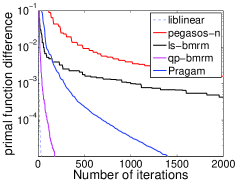
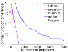
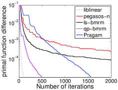
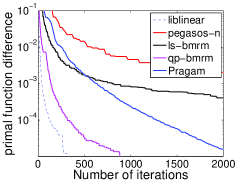
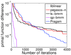
Figure 1: Primal function error versus number of iterations.

(a) astro-ph

(b) news20

(c) real-sim

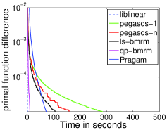
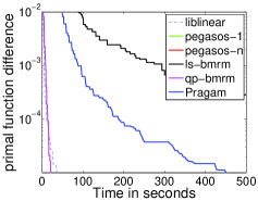
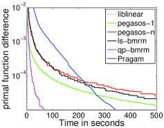
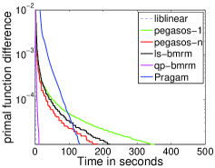
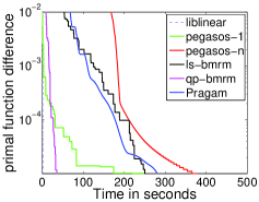
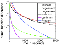
Figure 2: Primal function error versus time.

Due to lack of space, the figures of the detailed results are available in the Appendix D, and the main text only presents the results on three datasets.

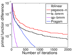
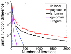
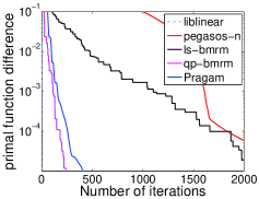
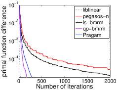
We first compared how fast ${\sf err}_{t}:=\min_{t^{\prime}<t}J(\mathbf{w}_{t^{\prime}})-J(\mathbf{w}^{*})$ decreases with respect to the iteration index $t$. We used ${\sf err}_{t}$ instead of $J(\mathbf{w}_{t})-J(\mathbf{w}^{*})$ because $J(\mathbf{w}_{t})$ in pegasos and ls-bmrm fluctuates drastically in some datasets. The results in Figure 1 show Pragam converges faster than ls-bmrm and pegasos-$n$ which both have $1/\varepsilon$ rates. liblinear converges much faster than the rest algorithms, and qp-bmrm is also fast. pegasos-1 is not included because it converges very slowly in terms of iterations.

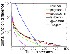
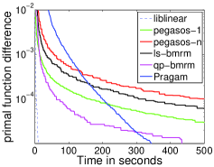
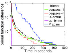
Next, we compared in Figure 2 how fast ${\sf err}_{t}$ decreases in wall clock time. Pragam is not fast in decreasing ${\sf err}_{t}$ to low accuracies like $10^{-3}$. But it becomes quite competitive when higher accuracy is desired, whereas ls-bmrm and pegasos-1 often take a long time in this case. Again, liblinear is much faster than the other algorithms.

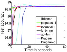
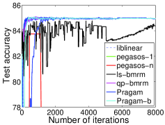
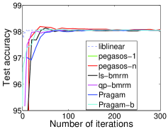
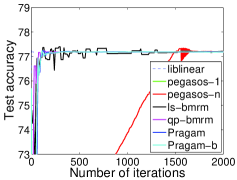
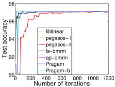
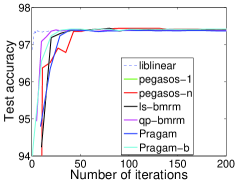
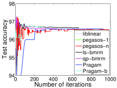
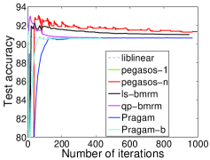
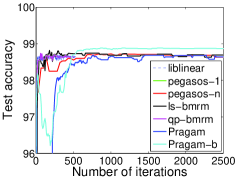
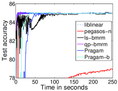
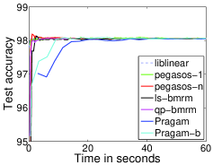
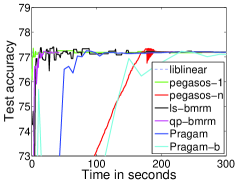
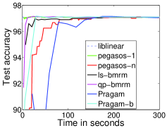
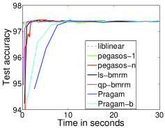
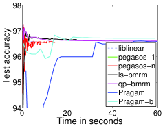
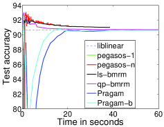
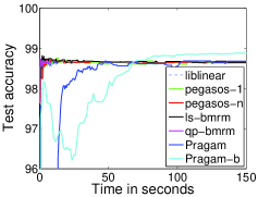
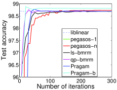
Another evaluation is on how fast a solver finds a model with reasonable accuracy. At iteration $t$, we examined the test accuracy of $\mathbf{w}_{t^{\prime}}$ where $t^{\prime}:=\mathop{\mathrm{argmin}}_{t^{\prime}\leq t}J(\mathbf{w}_{t^{\prime}})$, and the result is presented in Figures 3 and 4 with respect to number of iterations and time respectively. It can be seen that although Pragam manages to minimize the primal function fast, its generalization power is not improved efficiently. This is probably because this generalization performance hinges on the sparsity of the solution (or number of support vectors, [15]), and compared with all the other algorithms Pragam does not achieve any sparsity in the process of optimization. Asymptotically, all the solvers achieve very similar testing accuracy.

Since the objective function of Pragam-b has a different feasible region than other optimizers which do not use bias, we only compared its test accuracy. In Figures 3 and 4, the test accuracy of the optimal solution found by Pragam-b is always higher than or similar to that of the other solvers. In most cases, Pragam-b achieves the same test accuracy faster than Pragam both in number of iterations and time.

(a) astro-ph

(b) news20

(c) real-sim

Figure 3: Test accuracy versus number of iterations.

(a) astro-ph

(b) news20

(c) real-sim

Figure 4: Test accuracy versus time.

6 Discussion and Conclusions

In this paper we described a new lower bound for the number of iterations required by BMRM and similar algorithms which are widely used solvers for the regularized risk minimization problem. This shows that the iteration bounds shown for these solvers is optimum. Our lower bounds are somewhat surprising because the empirical performance of these solvers indicates that they converge linearly to an $\varepsilon$ accurate solution on a large number of datasets. Perhaps a more refined analysis is needed to explain this behavior.

The SVM problem has received significant research attention recently. For instance, [9] proposed a stochastic subgradient algorithm Pegasos. The convergence of Pegasos is analyzed in a stochastic setting and it was shown that it converges in $O(1/\varepsilon)$ iterations. We believe that our lower bounds can be extended to any arbitrary subgradient based solvers in the primal including Pegasos. This is part of ongoing research.

Our technique of solving the dual optimization problem is not new. A number of solvers including SVM-Light [16] and SMO [17] work on the dual problem. Even though linear convergence is established for these solvers, their rates have $n^{\geq 3}$ dependence which renders the analysis unusable for practical purposes. Other possible approaches include the interior-point method of [18] which costs $O(nd^{2}\log(\log(1/\varepsilon)))$ time and $O(d^{2})$ space where $d$ refers to the dimension of the features. LibLinear [11] performs coordinate descent in the dual, and has $O(nd\log(1/\varepsilon))$ complexity but only after more than $O(n^{2})$ steps. Mirror descent algorithms [19] cost $O(nd)$ per iteration, but their convergence rate is $1/\varepsilon^{2}$. These rates are prohibitively expensive when $n$ is very large.

The $O(1/\sqrt{\varepsilon})$ rates for the new SVM algorithm we described in this paper has a favorable dependence on $n$ as well as $\lambda$. Although our emphasis has been largely theoretical, the empirical experiments indicate that our solver is competitive with the state of the art. Finding an efficient solver with fast rates of convergence and good empirical performance remains a holy grail of optimization for machine learning.

Appendix

Appendix A Minimax Theorem on Convex spaces

The reversal of $\min$ and $\max$ operators in (3) follows from the following theorem. (Theorem 3 in [20])

Theorem 8

Let $X$ be a convex space, $Y$ a Hausdorff compact convex space and $f:X\times Y\to Z$ a function. Suppose that

• there is a subset $U\subset Z$ such that $a,b\in f(X\times Y)$ with $a<b$ implies $U\cap(a,b)\neq\emptyset$;

• $f(x,\cdot)$ is lower semicontinuous ($l.s.c.$) on $Y$ and $\left\{y\in Y:f(x,y)<s\right\}$ is convex for each $x\in X$ and $s\in U$ and

• $f(\cdot,y)$ is upper semicontinuous ($u.s.c.$) on $X$ and $\left\{x\in X:f(x,y)<s\right\}$ is convex for each $y\in Y$ and $s\in U$

Then

$$\max_{x\in X}\min_{y\in Y}f(x,y)=\min_{y\in Y}\max_{x\in X}f(x,y)$$

It is trivial to show that our setting satisfies the above three conditions for the linear form $f(\mathbf{w},\bm{\alpha})=\mathbf{w}^{\top}\mathbf{A}_{t}\bm{\alpha}$.

In our case $Z=\mathbb{R}$. Since $\alpha\in\Delta_{t}$ and the columns of $\mathbf{A}$ have Euclidean norm 1, it can be easily shown that $w$ is bounded in a ball of radius $1/\lambda$. Thus the range space is a finite subset of $\mathbb{R}$ and we choose $U$ to be the entire range space so that it will satisfy the first condition as $f(\mathbf{w},\bm{\alpha})$ is a continuous function.

Also $g(\bm{\alpha})=f(\mathbf{w},\bm{\alpha})$ and $h(\mathbf{w})=f(\mathbf{w},\bm{\alpha})$ are continuous functions in $\bm{\alpha}$ and $\mathbf{w}$ respectively and are thus by definition lower (upper) semicontinuous in $\bm{\alpha}$ ($\mathbf{w}$). The convexity of the sets in the $2^{nd}$ and $3^{rd}$ condition follows from first principles using definition of convexity. Thus we can use the minimax theorem to obtain (3).

Appendix B A linear time algorithm for a box constrained diagonal QP with a single linear equality constraint

It can be shown that the dual optimization problem $D(\bm{\alpha})$ from (20) can be reduced into a box constrained QP with a single linear equality constraint.

In this section, we focus on the following simple QP:

$$\min\frac{1}{2}\sum_{i=1}^{n} d_{i}^{2}(\alpha_{i}-m_{i})^{2}$$

$$s.t.\qquad l_{i}\leq \alpha_{i}\leq u_{i}\quad\forall i\in[n];$$

$$\sum_{i=1}^{n} \sigma_{i}\alpha_{i}=z.$$

Without loss of generality, we assume $l_{i}<u_{i}$ and $d_{i}\neq 0$ for all $i$. Also assume $\sigma_{i}\neq 0$ because otherwise $\alpha_{i}$ can be solved independently. To make the feasible region nonempty, we also assume

$$\sum_{i}\sigma_{i}(\delta(\sigma_{i}>0)l_{i}+\delta(\sigma_{i}<0)u_{i})\leq z\leq\sum_{i}\sigma_{i}(\delta(\sigma_{i}>0)u_{i}+\delta(\sigma_{i}<0)l_{i}).$$

The algorithm we describe below stems from [21] and finds the exact optimal solution in $O(n)$ time, faster than the $O(n\log n)$ complexity in [7].

With a simple change of variable $\beta_{i}=\sigma_{i}(\alpha_{i}-m_{i})$, the problem is simplified as $\displaystyle\min\qquad\frac{1}{2}\sum_{i=1}^{n}$ $\displaystyle\bar{d}^{2}_{i}\beta_{i}^{2}$ $\displaystyle s.t.\qquad l^{\prime}_{i}\leq$ $\displaystyle\beta_{i}\leq u^{\prime}_{i}\quad\forall i\in[n];$ $\displaystyle\sum_{i=1}^{n}$ $\displaystyle\beta_{i}=z^{\prime},$ where $\displaystyle l^{\prime}_{i}$ $\displaystyle=\left\{{\begin{array}[]{ll}\sigma_{i}(l_{i}-m_{i})&\text{if }\sigma_{i}>0\\ \sigma_{i}(u_{i}-m_{i})&\text{if }\sigma_{i}<0\\ \end{array}}\right.,$ $\displaystyle u^{\prime}_{i}$ $\displaystyle=\left\{{\begin{array}[]{ll}\sigma_{i}(u_{i}-m_{i})&\text{if }\sigma_{i}>0\\ \sigma_{i}(l_{i}-m_{i})&\text{if }\sigma_{i}<0\\ \end{array}}\right.,$ $\displaystyle\bar{d}^{2}_{i}$ $\displaystyle=\frac{d_{i}^{2}}{\sigma_{i}^{2}},\quad z^{\prime}=z-\sum_{i}\sigma_{i}m_{i}.$

We derive its dual via the standard Lagrangian.

$$L=\frac{1}{2}\sum_{i}\bar{d}^{2}_{i}\beta_{i}^{2}-\sum_{i}\rho_{i}^{+}(\beta_{i}-l^{\prime}_{i})+\sum_{i}\rho_{i}^{-}(\beta_{i}-u^{\prime}_{i})-\lambda\left(\sum_{i}\beta_{i}-z^{\prime}\right).$$

Taking derivative:

$$\frac{\partial L}{\partial\beta_{i}}=\bar{d}^{2}_{i}\beta_{i}-\rho_{i}^{+}+\rho_{i}^{-}-\lambda=0\quad\Rightarrow\quad\beta_{i}=\bar{d}^{-2}_{i}(\rho_{i}^{+}-\rho_{i}^{-}+\lambda).$$ (27)

Substituting into $L$, we get the dual optimization problem

$$\min D(\lambda,\rho_{i}^{+},\rho_{i}^{-}) =\frac{1}{2}\sum_{i}\bar{d}^{-2}_{i}(\rho_{i}^{+}-\rho_{i}^{-}+\lambda)^{2}-\sum_{i}\rho_{i}^{+}l^{\prime}_{i}+\sum_{i}\rho_{i}^{+}u^{\prime}_{i}-\lambda z^{\prime}$$

$$s.t.\qquad \rho_{i}^{+}\geq 0,\quad\rho_{i}^{-}\geq 0\quad\forall i\in[n].$$

Taking derivative of $D$ with respect to $\lambda$, we get:

$$\sum_{i}\bar{d}^{-2}_{i}(\rho_{i}^{+}-\rho_{i}^{-}+\lambda)-z^{\prime}=0.$$ (28)

The KKT condition gives:

$$\rho_{i}^{+}(\beta_{i}-l^{\prime}_{i}) =0,$$ (29a)

$$\rho_{i}^{-}(\beta_{i}-u^{\prime}_{i}) =0.$$ (29b)

Now we enumerate four cases.

1. $\rho_{i}^{+}>0$, $\rho_{i}^{-}>0$.

This implies that $l^{\prime}_{i}=\beta_{i}=u^{\prime}_{i}$, which is contradictory to our assumption.

2. $\rho_{i}^{+}=0$, $\rho_{i}^{-}=0$.

Then by (27), $\beta_{i}=\bar{d}^{-2}_{i}\lambda\in[l^{\prime}_{i},u^{\prime}_{i}]$, hence $\lambda\in[\bar{d}^{2}_{i}l^{\prime}_{i},\bar{d}^{2}_{i}u^{\prime}_{i}]$.

3. $\rho_{i}^{+}>0$, $\rho_{i}^{-}=0$.

Now by (29) and (27), we have $l^{\prime}_{i}=\beta_{i}=\bar{d}^{-2}_{i}(\rho_{i}^{+}+\lambda)>\bar{d}^{-2}_{i}\lambda$, hence $\lambda<\bar{d}^{2}_{i}l^{\prime}_{i}$ and $\rho_{i}^{+}=\bar{d}^{2}_{i}l^{\prime}_{i}-\lambda$.

4. $\rho_{i}^{+}=0$, $\rho_{i}^{-}>0$.

Now by (29) and (27), we have $u^{\prime}_{i}=\beta_{i}=\bar{d}^{-2}_{i}(-\rho_{i}^{-}+\lambda)<\bar{d}^{-2}_{i}\lambda$, hence $\lambda>\bar{d}^{2}_{i}u^{\prime}_{i}$ and $\rho_{i}^{-}=-\bar{d}^{2}_{i}u^{\prime}_{i}+\lambda$.

In sum, we have $\rho_{i}^{+}=[\bar{d}^{2}_{i}l^{\prime}_{i}-\lambda]_{+}$ and $\rho_{i}^{-}=[\lambda-\bar{d}^{2}_{i}u^{\prime}_{i}]_{+}$. Now (28) turns into

$$f(\lambda):=\sum_{i}\underbrace{\bar{d}^{-2}_{i}([\bar{d}^{2}_{i}l^{\prime}_{i}-\lambda]_{+}-[\lambda-\bar{d}^{2}_{i}u^{\prime}_{i}]_{+}+\lambda)}_{=:h_{i}(\lambda)}-z^{\prime}=0.$$ (30)

In other words, we only need to find the root of $f(\lambda)$ in (30). $h_{i}(\lambda)$ is plotted in Figure 5. Note that $h_{i}(\lambda)$ is a monotonically increasing function of $\lambda$, so the whole $f(\lambda)$ is monotonically increasing in $\lambda$. Since $f(\infty)\geq 0$ by $z^{\prime}\leq\sum_{i}u^{\prime}_{i}$ and $f(-\infty)\leq 0$ by $z^{\prime}\geq\sum_{i}l^{\prime}_{i}$, the root must exist. Considering that $f$ has at most $2n$ kinks (nonsmooth points) and is linear between two adjacent kinks, the simplest idea is to sort $\left\{\bar{d}^{2}_{i}l^{\prime}_{i},\bar{d}^{2}_{i}u^{\prime}_{i}:i\in[n]\right\}$ into $s^{(1)}\leq\ldots\leq s^{(2n)}$. If $f(s^{(i)})$ and $f(s^{(i+1)})$ have different signs, then the root must lie between them and can be easily found because $f$ is linear in $[s^{(i)},s^{(i+1)}]$. This algorithm takes at least $O(n\log n)$ time because of sorting.

Figure 5: $h_{i}(\lambda)$

However, this complexity can be reduced to $O(n)$ by making use of the fact that the median of $n$ (unsorted) elements can be found in $O(n)$ time. Notice that due to the monotonicity of $f$, the median of a set $S$ gives exactly the median of function values, i.e., $f({\text{MED}}(S))={\text{MED}}(\left\{f(x):x\in S\right\})$. Algorithm 2 sketches the idea of binary search. The while loop terminates in $\log_{2}(2n)$ iterations because the set $S$ is halved in each iteration. And in each iteration, the time complexity is linear to $|S|$, the size of current $S$. So the total complexity is $O(n)$. Note the evaluation of $f(m)$ potentially involves summing up $n$ terms as in (30). However by some clever aggregation of slope and offset, this can be reduced to $O(|S|)$.

1:  Set kink set $S\leftarrow\left\{\bar{d}_{i}^{2}l^{\prime}_{i}:i\in[n]\right\}\cup\left\{\bar{d}_{i}^{2}u^{\prime}_{i}:i\in[n]\right\}$.

2:  while $\left|S\right|>2$ do

3:     Find median of $S$: $m\leftarrow{\text{MED}}(S)$.

4:     if $f(m)\geq 0$ then

5:        $S\leftarrow\left\{x\in S:x\leq m\right\}$.

6:     else

7:        $S\leftarrow\left\{x\in S:x\geq m\right\}$.

8:     end if

9:  end while

10:  Return root $\frac{lf(u)-uf(l)}{f(u)-f(l)}$ where $S=\left\{l,u\right\}$.

Algorithm 2 $O(n)$ algorithm to find the root of $f(\lambda)$. Ignoring boundary condition checks.

Appendix C Derivation of $g^{\star}(\bm{\alpha})$

To see $g^{\star}(\bm{\alpha})=\min_{b\in\mathbb{R}}\frac{1}{n}\sum_{i}\left[1+\alpha_{i}-y_{i}b\right]_{+}$ in (20), it suffices to show that for all $\bm{\alpha}\in\mathbb{R}^{n}$:

$$\sup_{\bm{\rho}\in Q_{2}}\left\langle\bm{\rho},\bm{\alpha}\right\rangle+\sum_{i}\rho_{i}=\min_{b\in\mathbb{R}}\frac{1}{n}\sum_{i}\left[1+\alpha_{i}-y_{i}b\right]_{+}.$$ (31)

Posing the latter optimization as:

$$\min_{\xi_{i},b}\frac{1}{n}\sum_{i}\xi_{i}\qquad s.t.\quad 1+\alpha_{i}-y_{i}b\leq\xi_{i},\quad\xi_{i}\geq 0.$$

Write out the Lagrangian:

$$L=\frac{1}{n}\sum_{i}\xi_{i}+\sum_{i}\rho_{i}(1+\alpha_{i}-y_{i}b-\xi_{i})-\sum_{i}\beta_{i}\xi_{i}.$$

Taking partial derivatives:

$$\frac{\partial L}{\partial\xi_{i}} =\frac{1}{n}-\rho_{i}-\beta_{i}=0\qquad \Rightarrow \qquad\rho_{i}\in[0,n^{-1}],$$

$$\frac{\partial L}{\partial b} =-\sum_{i}\rho_{i}y_{i}=0\qquad \Rightarrow \qquad\sum_{i}\rho_{i}y_{i}=0.$$

Plugging back into $L$,

$$L=\sum_{i}\rho_{i}(1+\alpha_{i}),\qquad\text{s.t. }\quad\rho_{i}\in[0,n^{-1}],\quad\sum_{i}\rho_{i}y_{i}=0.$$

Maximizing $L$ wrt $\bm{\rho}$ is exactly the LHS of (31).

Appendix D Experimental Results in Detail

The $\lambda$s used in the experiment are:

dataset	$\lambda$	dataset	$\lambda$	dataset	$\lambda$	dataset	$\lambda$
adult	$2^{-18}$	astro-ph	$2^{-17}$	aut-avn	$2^{-17}$	covertype	$2^{-17}$
news20	$2^{-14}$	reuters-c11	$2^{-19}$	reuters-ccat	$2^{-19}$	real-sim	$2^{-16}$
web8	$2^{-17}$

(a) adult9 (pegasos diverged)

(b) astro-ph

(c) aut-avn

(d) covertype

(e) news20

(f) real-sim

(g) reuters-c11

(h) reuters-ccat

(i) web8

Figure 6: Primal function error versus number of iterations.

(a) adult9 (pegasos diverged)

(b) astro-ph

(c) aut-avn

(d) covertype

(e) news20

(f) real-sim

(g) reuters-c11

(h) reuters-ccat

(i) web8

Figure 7: Primal function error versus time.

(a) adult9

(b) astro-ph

(c) aut-avn

(d) covertype

(e) news20

(f) real-sim

(g) reuters-c11

(h) reuters-ccat

(i) web8

Figure 8: Test accuracy versus number of iterations.

(a) adult9

(b) astro-ph

(c) aut-avn

(d) covertype

(e) news20

(f) real-sim

(g) reuters-c11

(h) reuters-ccat

(i) web8

Figure 9: Test accuracy versus time.

Appendix E Structured Output

In this section, we show how Pragam can be applied to structured output data. When the output space $\mathbf{y}$ has structures, the label space becomes exponentially large and the problem becomes much more expensive. To make the computation tractable, it is common to reparameterize on the cliques and to estimate the parameters via graphical model inference. We Below are two examples.

E.1 Margin Scaled Maximum Margin Markov Network

The maximum margin Markov network formulation (M³N) by [22] has the following dual form (skipping the primal). Here, a training example $i$ has a graphical model with maximal clique set $\mathcal{C}^{(i)}$. For each $i$ and $c\in\mathcal{C}^{(i)}$, $\alpha_{i,c}(\mathbf{y}_{c})$ stands for the marginal probability of the clique configuration $\mathbf{y}_{c}$. Any possible structured output $\mathbf{y}$ can be measured against the given true label $\mathbf{y}^{i}$ with a loss function $\ell_{i}(\mathbf{y})$. It is assumed that $\ell_{i}(\mathbf{y})$ decomposes additively onto the cliques: $\ell_{i}(\mathbf{y})=\sum_{c\in\mathcal{C}^{(i)}}\ell_{i,c}(\mathbf{y}_{c})$. In addition, [22] uses a joint feature map $\mathbf{f}_{i}(\mathbf{y}):=\mathbf{f}(\mathbf{x}^{i},\mathbf{y})$, and define $\Delta\mathbf{f}_{i}(\mathbf{y}):=\mathbf{f}_{i}(\mathbf{y}^{i})-\mathbf{f}_{i}(\mathbf{y})$. Again, we assume that $\mathbf{f}_{i}(\mathbf{y})$ decomposes additively onto the cliques: $\mathbf{f}_{i}(\mathbf{y})=\sum_{c}\mathbf{f}_{i,c}(\mathbf{y}_{c})$, where $\mathbf{f}_{i,c}(\mathbf{y}_{c}):=\mathbf{f}_{c}(\mathbf{x}^{i},\mathbf{y}_{c})$. The simplest joint feature map is defined by:

$$\left\langle\mathbf{f}_{c}(\mathbf{x},\mathbf{y}_{c}),\mathbf{f}_{c^{\prime}}(\bar{\mathbf{x}},\bar{\mathbf{y}}_{c^{\prime}})\right\rangle=\delta(\mathbf{y}_{c}=\bar{\mathbf{y}}_{c^{\prime}})k(\mathbf{x}_{c},\bar{\mathbf{x}}_{c^{\prime}})=\delta(\mathbf{y}_{c}=\bar{\mathbf{y}}_{c^{\prime}})\left\langle\mathbf{x}_{c},\bar{\mathbf{x}}_{c^{\prime}}\right\rangle.$$

Notice that $c$ and $c^{\prime}$ are not required to be of the same “type”, and $\delta(\mathbf{y}_{c}=\bar{\mathbf{y}}_{c^{\prime}})$ will automatically filter out incompatible types, e.g., $c$ is an edge and $c^{\prime}$ is a node. This kernel can be easily vectorized into $\mathbf{f}(\mathbf{x},\mathbf{y}):=\sum_{c}\left(\mathbf{x}_{c}\bigotimes(\delta(\mathbf{y}_{c}=\mathbf{y}_{c,1}),\ldots,\delta(\mathbf{y}_{c}=\mathbf{y}_{c,m(c)}))^{\top}\right)$, where $m(c)$ is the number of label configurations that clique $c$ can take, and $\bigotimes$ (cross product) is defined by:

$$\otimes:\mathbb{R}^{s}\times\mathbb{R}^{t}\to\mathbb{R}^{st},\qquad(\mathbf{a}\otimes\mathbf{b})_{(i-1)t+j}:=a_{i}b_{j}.$$

$$\min_{\bm{\alpha}}\qquad\frac{C}{2}\left\|\sum_{i,c,\mathbf{y}_{c}}\alpha_{i,c}(\mathbf{y}_{c})\Delta\mathbf{f}_{i,c}(\mathbf{y}_{c})\right\|^{2} -\sum_{i,c,\mathbf{y}_{c}}\alpha_{i,c}(\mathbf{y}_{c})\ell_{i,c}(\mathbf{y}_{c})$$

$$s.t.\qquad\qquad\qquad\quad\sum_{\mathbf{y}_{c}}\alpha_{i,c}(\mathbf{y}_{c}) =1\qquad\qquad\qquad\qquad\quad\forall i,\forall c\in\mathcal{C}^{(i)};$$

$$\alpha_{i,c}(\mathbf{y}_{c}) \geq 0\qquad\qquad\qquad\qquad\quad\forall i,\forall c\in\mathcal{C}^{(i)},\forall\mathbf{y}_{c};$$

$$\sum_{\mathbf{y}_{c}\sim\mathbf{y}_{c\cap c^{\prime}}}\alpha_{i,c}(\mathbf{y}_{c}) =\sum_{\mathbf{y}_{c^{\prime}}\sim\mathbf{y}_{c\cap c^{\prime}}}\alpha_{i,c^{\prime}}(\mathbf{y}_{c^{\prime}})\qquad\forall i,\forall c,c^{\prime}\in\mathcal{C}^{(i)}:c\cap c^{\prime}\neq\emptyset,\forall\mathbf{y}_{c\cap c^{\prime}}.$$

The subroutines of mapping in (23) and (25) can be viewed as projecting a vector onto the probability simplex under $L_{2}$ distance. Moreover, the image now is restricted to the pmf which satisfies the conditional independence properties encoded by the graphical model. This is much more difficult than projecting onto a box with a linear equality constraint as in SVM, and we can only resort to a block coordinate descent as detailed in Appendix E.3.

E.2 Gaussian Process Sequence Labeling

[23] proposed using Gaussian process to segment and annotate sequences. It assumes that all training sequences have the same length $l$, and each node can take values in $[m]$. For sequences, the maximum cliques are edges: $\mathcal{C}^{(i)}=\left\{(t,t+1):t\in[l-1]\right\}$. We use $\bm{\alpha}$ to stack up the marginal distributions on the cliques:

$$\left\{\alpha_{i,c}(\mathbf{y}_{c}):i,c\in\mathcal{C}^{(i)},\mathbf{y}_{c}\right\}=\left\{\alpha_{i,t}(y_{t},y_{t+1}):i,t\in[l-1],y_{t},y_{t+1}\in[m]\right\}.$$

The marginal probability $\alpha_{i,c}(\mathbf{y}_{c})$ just aggregates relevant elements in the joint distribution via a linear transform. With the joint distribution vector $p\in\mathbb{R}^{nm^{l}}$, we can write $\bm{\alpha}=\Lambda p$, where $\Lambda$ is $nlm^{2}\times nm^{l}$ defined by

$$\lambda_{(j,t,\sigma,\tau),(i,\mathbf{y})}=\delta(i=j\wedge y_{t}=\sigma\wedge y_{t+1}=\tau).$$

A key difference from the M³N is that in Gaussian process, the constraint that the joint density lying in the probability simplex is replaced by regularizing the log partition function. So the set of marginal distributions on cliques do not have local consistency constraints, i.e., they are free variables. The ultimate optimization problem in [23] is an unconstrained optimization:

$$\min_{\bm{\alpha}}\qquad\bm{\alpha}^{\top}K\bm{\alpha}-\sum_{i=1}^{n}\bm{\alpha}^{\top}K\Lambda e_{(e,\mathbf{y}_{i})}+\sum_{i=1}^{n}\log\sum_{\mathbf{y}}\exp\left(\bm{\alpha}^{\top}K\Lambda e_{i,\mathbf{y}}\right).$$ (32)

where $K$ is a kernel on $\left\{(\mathbf{x}^{i},(y^{i}_{t},y^{i}_{t+1})):i,t\in[l-1],y_{t},y_{t+1}\in[m]\right\}$. A simple example is:

$$k((\mathbf{x}^{i},(y^{i}_{t},y^{i}_{t+1})),(\mathbf{x}^{j},(y^{j}_{t^{\prime}},y^{j}_{t^{\prime}+1}))= \delta(t=t^{\prime})\left(\delta(y^{i}_{t}=y^{j}_{t^{\prime}}\wedge y^{i}_{t+1}=y^{j}_{t^{\prime}+1})+\right.$$

$$\left.k(\mathbf{x}^{i}_{t},\mathbf{x}^{j}_{t^{\prime}})\delta(y^{i}_{t}=y^{j}_{t^{\prime}})+k(\mathbf{x}^{i}_{t+1},\mathbf{x}^{j}_{t^{\prime}+1})\delta(y^{i}_{t+1}=y^{j}_{t^{\prime}+1})\right).$$

If stationality is assumed, we can drop the $\delta(t=t^{\prime})$ above and allow node swapping:

$$k((\mathbf{x}^{i},(y^{i}_{t},y^{i}_{t+1})),(\mathbf{x}^{j},(y^{j}_{t^{\prime}},y^{j}_{t^{\prime}+1}))= \delta(y^{i}_{t}=y^{j}_{t^{\prime}}\wedge y^{i}_{t+1}=y^{j}_{t^{\prime}+1})$$

$$+\sum_{p\in\left\{t,t+1\right\}}\sum_{q\in\left\{t^{\prime},t^{\prime}+1\right\}}k(\mathbf{x}^{i}_{p},\mathbf{x}^{j}_{q})\delta(y^{i}_{p}=y^{j}_{q}).$$

The gradient of the first two terms in (32) can be computed with ease. The gradient of the last term is

$${\nabla}_{\bm{\alpha}}\left[\log\sum_{\mathbf{y}}\exp\left(\bm{\alpha}^{\top}K\Lambda e_{i,\mathbf{y}}\right)\right]=K\mathbb{E}_{Y}\left[\Lambda e_{i,Y}\right].$$

[23] computes this expectation via the forward-backward algorithm. The projections (23) and (25) are the same as in Appendix E.1, and Appendix E.3.1 provides a solver for the special case of sequence.

E.3 Efficient projection onto $n$ dimensional simplex factorized by a graphical model

As a simple extension of Appendix B, we now consider a more involved case. In addition to projecting onto the $n$ dimensional simplex under $L_{2}$ distance, we also restrict that the image is factorized according to a graphical model. Formally, suppose we have a graphical model over $n$ random variables with maximum clique set $\mathcal{C}$. For each clique $c$, suppose the set of all its possible configuration is $V_{c}$, and the pmf of the marginal distribution on clique $c$ is $\alpha_{c}(\mathbf{y}_{c})$, where $\mathbf{y}_{c}\in V_{c}$. Given a set $\left\{\mathbf{m}_{c}\in\mathbb{R}^{\left|V_{c}\right|}:c\in\mathcal{C}\right\}$, we want to find a set $\left\{\bm{\alpha}_{c}\in\mathbb{R}^{\left|V_{c}\right|}:c\in\mathcal{C}\right\}$ which minimizes:

$$\min\qquad\frac{1}{2}\sum_{c}d_{c}^{2} \left\|\bm{\alpha}_{c}-\mathbf{m}_{c}\right\|_{2}^{2}$$

$$s.t.\qquad\sum_{\mathbf{y}_{c}}\alpha_{c}(\mathbf{y}_{c}) =1\qquad\qquad\forall c\in\mathcal{C};$$

$$\alpha_{c}(\mathbf{y}_{c}) \geq 0\qquad\qquad\forall c\in\mathcal{C},\forall\mathbf{y}_{c};$$

$$\sum_{\mathbf{y}_{c}\sim\mathbf{y}_{c\cap c^{\prime}}}\alpha_{c}(\mathbf{y}_{c}) =\sum_{\mathbf{y}_{c^{\prime}}\sim\mathbf{y}_{c\cap c^{\prime}}}\alpha_{c^{\prime}}(\mathbf{y}_{c^{\prime}})\quad\forall c\cap c^{\prime}\neq\emptyset,\forall\mathbf{y}_{c\cap c^{\prime}}.$$

The last (set of) constraint enforces the local consistency of the marginal distributions, and $\mathbf{y}_{c}\sim\mathbf{y}_{c\cap c^{\prime}}$ means the assignment of clique $c$ matches $\mathbf{y}_{c\cap c^{\prime}}$ on the subset $c\cap c^{\prime}$. If the graphical model is tree structured, then it will also guarantee global consistency. We proceed by writing out the standard Lagrangian:

$$L= \frac{1}{2}\sum_{c}d_{c}^{2}\sum_{\mathbf{y}_{c}}(\alpha_{c}(\mathbf{y}_{c})-m_{c}(\mathbf{y}_{c}))^{2}-\sum_{c}\lambda_{c}\left(\sum_{\mathbf{y}_{c}}\alpha_{c}(\mathbf{y}_{c})-1\right)-\sum_{c,\mathbf{y}_{c}}\xi_{c}(\mathbf{y}_{c})\alpha_{c}(\mathbf{y}_{c})$$

$$-\sum_{c,c^{\prime}:c\cap c^{\prime}\neq\emptyset}\sum_{\mathbf{y}_{c\cap c^{\prime}}}\bar{\mu}_{c,c^{\prime}}(\mathbf{y}_{c\cap c^{\prime}})\left(\sum_{\mathbf{y}_{c}:\mathbf{y}_{c}\sim\mathbf{y}_{c\cap c^{\prime}}}\alpha_{c}(\mathbf{y}_{c})-\sum_{\mathbf{y}_{c^{\prime}}\sim\mathbf{y}_{c\cap c^{\prime}}}\alpha_{c^{\prime}}(\mathbf{y}_{c^{\prime}})\right).$$

Taking derivative over $\alpha_{c}(y_{c})$:

$$\frac{\partial L}{\partial\alpha_{c}(\mathbf{y}_{c})} =d_{c}^{2}(\alpha_{c}(\mathbf{y}_{c})-m_{c}(\mathbf{y}_{c}))-\lambda_{c}-\xi_{c}(\mathbf{y}_{c})-\sum_{c^{\prime}}\bar{\mu}_{c,c^{\prime}}(\mathbf{y}_{c\cap c^{\prime}})+\sum_{c^{\prime}}\bar{\mu}_{c^{\prime},c}(\mathbf{y}_{c\cap c^{\prime}})=0,$$

$$\Rightarrow\alpha_{c}(\mathbf{y}_{c})=m_{c}(\mathbf{y}_{c})+d_{c}^{-2}\left(\lambda_{c}+\xi_{c}(\mathbf{y}_{c})+\sum_{c^{\prime}}\mu_{c,c^{\prime}}(\mathbf{y}_{c\cap c^{\prime}})\right),$$ (33)

where $\mu_{c,c^{\prime}}(\mathbf{y}_{c\cap c^{\prime}}):=\bar{\mu}_{c,c^{\prime}}(\mathbf{y}_{c\cap c^{\prime}})-\bar{\mu}_{c^{\prime},c}(\mathbf{y}_{c\cap c^{\prime}})$. Plugging it back into $L$, we derive the dual problem:

$$\min D(\lambda_{c},\xi_{c}(\mathbf{y}_{c}),\mu_{c,c^{\prime}}(\mathbf{y}_{c\cap c^{\prime}}))= \frac{1}{2}\sum_{c}d_{c}^{-2}\sum_{\mathbf{y}_{c}}\left(\lambda_{c}+\xi_{c}(\mathbf{y}_{c})+\sum_{c^{\prime}}\mu_{c,c^{\prime}}(\mathbf{y}_{c\cap c^{\prime}})\right)^{2}$$ (34)

$$+\sum_{c}\sum_{\mathbf{y}_{c}}m_{c}(\mathbf{y}_{c})\left(\lambda_{c}+\xi_{c}(\mathbf{y}_{c})+\sum_{c^{\prime}}\mu_{c,c^{\prime}}(\mathbf{y}_{c\cap c^{\prime}})\right)-\sum_{c}\lambda_{c}$$

$$s.t.\qquad\xi_{c}(\mathbf{y}_{c})\geq 0.$$

Looking at the problem, it is essentially a QP over $\lambda_{c},\xi_{c}(\mathbf{y}_{c}),\mu_{c,c^{\prime}}(\mathbf{y}_{c\cap c^{\prime}})$ with the only constraint that $\xi_{c}(\mathbf{y}_{c})\geq 0$. Similar to B, one can write $\xi_{c}(\mathbf{y}_{c})$ as a hinge function of $\lambda_{c}$ and $\mu_{c,c^{\prime}}(\mathbf{y}_{c\cap c^{\prime}})$. However since it is no longer a single variable function, it is very hard to apply the median trick here. So we resort to a simple block coordinate descent. The optimization steps are given in Algorithm 3 with reference to the following expressions of gradient:

$$\frac{\partial D}{\partial\xi_{c}(\mathbf{y}_{c})} =-d_{c}^{-2}(\lambda_{c}+\xi_{c}(\mathbf{y}_{c})+\sum_{c^{\prime}}\mu_{c,c^{\prime}}(\mathbf{y}_{c\cap c^{\prime}}))+m_{c}(\mathbf{y}_{c})=0$$ (35a)

$$\frac{\partial D}{\partial\lambda_{c}} =d_{c}^{-2}\sum_{\mathbf{y}_{c}}\left(\lambda_{c}+\xi_{c}(\mathbf{y}_{c})+\sum_{c^{\prime}}\mu_{c,c^{\prime}}(\mathbf{y}_{c\cap c^{\prime}})\right)+\sum_{\mathbf{y}_{c}}m_{c}(\mathbf{y}_{c})-1$$ (35b)

$$\frac{\partial D}{\partial\mu_{c,c^{\prime}}(\mathbf{y}_{c\cap c^{\prime}})} =d_{c}^{-2}\sum_{\mathbf{y}^{\prime}_{c}\sim\mathbf{y}_{c\cap c^{\prime}}}\left(\lambda_{c}+\xi_{c}(\mathbf{y}^{\prime}_{c})+\sum_{\bar{c}}\mu_{c,\bar{c}}(\mathbf{y}^{\prime}_{c,\bar{c}})\right)+\sum_{\mathbf{y}^{\prime}_{c}\sim\mathbf{y}_{c\cap c^{\prime}}}m_{c}(\mathbf{y}^{\prime}_{c}).$$ (35c)

From (35a) and $\xi_{c}(\mathbf{y}_{c})\geq 0$, we can derive

$$\xi_{c}(\mathbf{y}_{c})=\left[-d_{c}^{2}m_{c}(\mathbf{y}_{c})-\lambda_{c}-\sum_{c^{\prime}}\mu_{c,c^{\prime}}(y_{c\cap c^{\prime}})\right]_{+}.$$ (36)

1:  Randomly initialize $\left\{\lambda_{c}:c\right\},\left\{\xi_{c}(\mathbf{y}_{c}):c,\mathbf{y}_{c}\right\},\left\{\mu_{c,c^{\prime}}(\mathbf{y}_{c\cap c^{\prime}}):c,c^{\prime},\mathbf{y}_{c\cap c^{\prime}}\right\}$.

2:  while not yet converged do

3:     Fixing $\xi_{c}(\mathbf{y}_{c})$, apply conjugate gradient to minimize the unconstrained quadratic form in (34) with respect to $\left\{\lambda_{c}:c\right\}$ and $\left\{\mu_{c,c^{\prime}}(\mathbf{y}_{c\cap c^{\prime}}):c,c^{\prime},\mathbf{y}_{c\cap c^{\prime}}\right\}$. The necessary gradients are given in (35b) and (35c).

4:     Set $\xi_{c}(\mathbf{y}_{c})\leftarrow\left[-d_{c}^{2}m_{c}(\mathbf{y}_{c})-\lambda_{c}-\sum_{c^{\prime}}\mu_{c,c^{\prime}}(y_{c\cap c^{\prime}})\right]_{+}$ for all $c\in\mathcal{C}$ and $\mathbf{y}_{c}$.

5:  end while

6:  Compute $\alpha_{c}(\mathbf{y}_{c})$ according to (33).

Algorithm 3 A coordinate descent scheme for minimizing the dual problem (34).

E.3.1 Special case: sequence

Suppose the graph is simply a sequence: $x_{1}-x_{2}-\ldots-x_{L}$ and each node can take value in $[m]$. Then the cliques are $\left\{(x_{t},x_{t+1}):t\in[L-1]\right\}$ and the primal is:

$$\min\qquad\frac{1}{2}\sum_{t=1}^{L-1}d_{t}^{2}\sum_{i,j=1}^{m} (\alpha_{t}(i,j)-m_{t}(i,j))^{2}$$

$$s.t.\qquad\sum_{i,j}\alpha_{t}(i,j) =1\qquad \forall t\in[L-1];$$

$$\alpha_{t}(i,j) \geq 0\qquad \forall t\in[L-1],i,j\in[m];$$

$$\sum_{i}\alpha_{t}(i,j) =\sum_{k}\alpha_{t+1}(j,k)\qquad \forall t\in[L-2],j\in[m].$$

Proceeding with the standard Lagrangian:

$$L= \sum_{t=1}^{L-1}d_{t}^{2}\sum_{i,j=1}^{m}(\alpha_{t}(i,j)-m_{t}(i,j))^{2}-\sum_{t=1}^{L-1}\lambda_{t}\left(\sum_{i,j}\alpha_{t}(i,j)-1\right)-\sum_{t=1}^{L-1}\sum_{i,j}\xi_{t}(i,j)\alpha_{t}(i,j)$$

$$-\sum_{t=1}^{L-2}\sum_{j}\mu_{t}(j)\left(\sum_{i}\alpha_{t}(i,j)-\sum_{k}\alpha_{t+1}(j,k)\right).$$

Taking derivative over $\alpha_{t}(i,j)$:

$$\frac{\partial L}{\partial\alpha_{t}(i,j)} =d_{t}^{2}(\alpha_{t}(i,j)-m_{t}(i,j))-\lambda_{t}-\xi_{t}(i,j)-\mu_{t}(j)+\mu_{t-1}(i)=0$$

$$\Rightarrow\alpha_{t}(i,j)=d_{t}^{-2}(\lambda_{t}+\xi_{t}(i,j)+\mu_{t}(j)-\mu_{t-1}(i))+m_{t}(i,j),$$ (37)

where we define $\mu_{0}(j):=0$. Plugging into $L$, we derive the dual problem:

$$\min D(\lambda_{t},\xi_{t}(i,j),\mu_{t}(i))= \frac{1}{2}\sum_{t=1}^{L-1}d_{t}^{2}\sum_{i,j}(\lambda_{t}+\xi_{t}(i,j)+\mu_{t}(j)-\mu_{t-1}(i))^{2}$$ (38)

$$+\sum_{t=1}^{L-1}\sum_{i,j}m_{t}(i,j)(\lambda_{t}+\xi_{t}(i,j)+\mu_{t}(j)-\mu_{t-1}(i))-\sum_{t=1}^{L-1}\lambda_{t}$$

$$s.t.\qquad\xi_{t}(i,j) \geq 0.\quad\forall t\in[L-1],\,i,j\in[m].$$

$$\frac{\partial D}{\partial\xi_{t}(i,j)} =d_{t}^{-2}(\lambda_{t}+\xi_{t}(i,j)+\mu_{t}(j)-\mu_{t-1}(i))+m_{t}(i,j)=0\qquad\qquad\qquad\quad\forall t\in[L-1]$$

$$\Rightarrow\xi_{t}(i,j)=[-d_{t}^{2}m_{t}(i,j)-\lambda_{t}-\mu_{t}(j)+\mu_{t-1}(i)]_{+}$$

$$\frac{\partial D}{\partial\lambda_{t}} =d_{t}^{-2}\sum_{i,j}(\lambda_{t}+\xi_{t}(i,j)+\mu_{t}(j)-\mu_{t-1}(i))+\sum_{i,j}m_{t}(i,j)-1\qquad\qquad\forall t\in[L-1]$$

$$\frac{\partial D}{\partial\mu_{t}(i)} =d_{t}^{-2}\sum_{j}(\lambda_{t}+\xi_{t}(j,i)+\mu_{t}(i)-\mu_{t-1}(j))\qquad\qquad\qquad\qquad\qquad\qquad\forall t\in[L-2]$$

$$\phantom{=}+d_{t+1}^{-2}\sum_{j}(\lambda_{t+1}+\xi_{t+1}(i,j)+\mu_{t+1}(j)-\mu_{t}(i))+\sum_{j}m_{t}(j,i)-\sum_{j}m_{t+1}(i,j),$$

where we further define $\mu_{L-1}(j):=0$. Obviously it takes $O(Lm^{2})$ to compute all the gradients, and so is $\left\{\xi_{t}(i,j)\right\}$.

References

• [1] I.Β Tsochantaridis, T.Β Joachims, T.Β Hofmann, and Y.Β Altun. Large margin methods for structured and interdependent output variables. J. Mach. Learn. Res., 6:1453–1484, 2005.
• [2] Alex Smola, S.Β V.Β N. Vishwanathan, and Quoc Le. Bundle methods for machine learning. In Daphne Koller and Yoram Singer, editors, Advances in Neural Information Processing Systems 20, Cambridge MA, 2007. MIT Press.
• [3] Yurri Nesterov. A method for unconstrained convex minimization problem with the rate of convergence O𝑂O(1/k2)1superscriptπ‘˜2(1/k^{2}). Soviet Math. Docl., 269:543–547, 1983.
• [4] J.B. Hiriart-Urruty and C.Β LemarΓ©chal. Convex Analysis and Minimization Algorithms, I and II, volume 305 and 306. Springer-Verlag, 1993.
• [5] ChoonΒ Hui Teo, S.Β V.Β N. Vishwanthan, AlexΒ J. Smola, and QuocΒ V. Le. Bundle methods for regularized risk minimization. J. Mach. Learn. Res., 2009. Submitted in February 2009.
• [6] Yurii Nesterov. Excessive gap technique in nonsmooth convex minimization. SIAM J. on Optimization, 16(1):235–249, 2005.
• [7] John Duchi, Shai Shalev-Shwartz, Yoram Singer, and Tushar Chandrae. Efficient projections onto the β„“1subscriptβ„“1\ell_{1}-ball for learning in high dimensions. In ICML, 2008.
• [8] J.Β M. Borwein and A.Β S. Lewis. Convex Analysis and Nonlinear Optimization: Theory and Examples. CMS books in Mathematics. Canadian Mathematical Society, 2000.
• [9] Shai Shalev-Shwartz, Yoram Singer, and Nathan Srebro. Pegasos: Primal estimated sub-gradient solver for SVM. In Proc.Β Intl.Β Conf.Β Machine Learning, 2007.
• [10] T.Β Joachims. Training linear SVMs in linear time. In Proc.Β ACM Conf.Β Knowledge Discovery and Data Mining (KDD). ACM, 2006.
• [11] ChoΒ Jui Hsieh, KaiΒ Wei Chang, ChihΒ Jen Lin, S.Β Sathiya Keerthi, and S.Β Sundararajan. A dual coordinate descent method for large-scale linear SVM. In William Cohen, Andrew McCallum, and Sam Roweis, editors, ICML, pages 408–415. ACM, 2008.
• [12] JoΒ A.Β M. Bollen. Numerical stability of descent methods for solving linear equations. Numerische Mathematik, 1984.
• [13] T.Β Joachims. A support vector method for multivariate performance measures. In Proc.Β Intl.Β Conf.Β Machine Learning, pages 377–384, San Francisco, California, 2005. Morgan Kaufmann Publishers.
• [14] Yurii Nesterov. Gradient methods for minimizing composite objective function. Technical ReportΒ 76, CORE Discussion Paper, UCL, 2007.
• [15] T.Β Graepel, R.Β Herbrich, and J.Β Shawe-Taylor. Generalisation error bounds for sparse linear classifiers. In Proc.Β Annual Conf.Β Computational Learning Theory, pages 298–303, 2000.
• [16] T.Β Joachims. Making large-scale SVM learning practical. In B.Β SchΓΆlkopf, C.Β J.Β C. Burges, and A.Β J. Smola, editors, Advances in Kernel Methods — Support Vector Learning, pages 169–184, Cambridge, MA, 1999. MIT Press.
• [17] J.Β Platt. Fast training of support vector machines using sequential minimal optimization. In B.Β SchΓΆlkopf, C.Β J.Β C. Burges, and A.Β J. Smola, editors, Advances in Kernel Methods — Support Vector Learning, pages 185–208, Cambridge, MA, 1999. MIT Press.
• [18] MichaelΒ C. Ferris and ToddΒ S. Munson. Interior-point methods for massive support vector machines. SIAM Journal on Optimization, 13(3):783–804, 2002.
• [19] Amir Beck and Marc Teboulle. Mirror descent and nonlinear projected subgradient methods for convex optimization. Operations Research Letters, 31(3):167–175, 2003.
• [20] Sehie Park. Minimax theorems in convex spaces. Novi Sad Journal of Mathematics, 28(2):1–8, 1998.
• [21] P.Β M. Pardalos and N.Β Kovoor. An algorithm for singly constrained class of quadratic programs subject to upper and lower bounds. Mathematical Programming, 46:321–328, 1990.
• [22] B.Β Taskar, C.Β Guestrin, and D.Β Koller. Max-margin Markov networks. In S.Β Thrun, L.Β Saul, and B.Β SchΓΆlkopf, editors, Advances in Neural Information Processing Systems 16, pages 25–32, Cambridge, MA, 2004. MIT Press.
• [23] Y.Β Altun, T.Β Hofmann, and A.Β J. Smola. Gaussian process classification for segmenting and annotating sequences. In Proc.Β Intl.Β Conf.Β Machine Learning, pages 25–32, New York, NY, 2004. ACM Press.