Improved simulation of non–Gaussian temperature and polarization CMB maps
Abstract
We describe an algorithm to generate temperature and polarization maps of the cosmic microwave background radiation containing non–Gaussianity of arbitrary local type. We apply an optimized quadrature scheme that allows us to predict and control integration accuracy, speed up the calculations, and reduce memory consumption by an order of magnitude. We generate 1000 non–Gaussian CMB temperature and polarization maps up to a multipole moment of . We validate the method and code using the power spectrum and the fast cubic (bispectrum) estimator and find consistent results. The simulations are provided to the community111Available at http://planck.mpa-garching.mpg.de/cmb/fnl-simulations.
1 Introduction
The simplest models of inflation predict almost perfectly Gaussian primordial fluctuations, generated by a single scalar quantum field in ground state (Guth 1981; Bardeen et al. 1983; Mukhanov et al. 1992), but a large number of alternative scenarios can easily be constructed. To test competing inflationary models, measurements of statistical properties of the cosmic microwave background (CMB) radiation have turned out to be of particular importance. Combined with constraints on the scalar spectral index and the search for gravitational waves imprinted on the polarization signature, the test for non–Gaussianity is a fundamental means to probe the physical processes of inflation.
Among all inflationary models predicting significant levels of non–Gaussianity, two broad classes can be distinguished. Non–Gaussianity of equilateral type is realized primarily in models with non–minimal Lagrangian including higher order derivatives (Alishahiha et al. 2004; Senatore 2005; Chen 2005; Langlois et al. 2008). Non–Gaussianity of local type is achieved to very good approximation in multi–field inflation (Moroi & Takahashi 2001; Enqvist & Sloth 2002; Lyth et al. 2003), or in cyclic/ekpyrotic universe models (Khoury et al. 2001; Steinhardt & Turok 2002; Lehners & Steinhardt 2008).
Concentrating on local non–Gaussianity, we parameterize the primordial curvature perturbations, , by introducing an additional quadratic dependence on a purely Gaussian auxiliary field , that is local in real space, of the form (Verde et al. 2000; Komatsu & Spergel 2001)
| (1) |
where is defined as
| (2) |
and is the dimensionless measure of the amplitude of non–Gaussianity. Primordial non–Gaussianity in the curvature perturbations will be encoded in the CMB signal.
Simulations of maps containing non–Gaussianity of local type have been extensively used in the context of WMAP data analysis. They play a crucial role in probing the sensitivity of analysis tools and provide the opportunity to quantitatively estimate the contribution of secondary anisotropies or instrumental effects to the measured level of non–Gaussianity in experimental data. With the advent of Planck, probing the non–Gaussian contribution within the CMB radiation even more accurately, the requirements for high resolution, high accuracy simulations of non–Gaussian CMB temperature and polarization maps will further increase.
To meet the demand for simulated non–Gaussian maps, several different approaches have been taken. First simulations of temperature maps with primordial non–Gaussianity of local type have generated the underlying primordial perturbation in Fourier space (Komatsu et al. 2003). This approach is computationally very demanding while it is difficult to preserve numerical accuracy. A different method has been proposed in Liguori et al. (2003, 2007), where the authors work with ‘filter’ functions to introduce the proper spatial correlations of the primordial potential. Recently, a fast, specifically tailored algorithm for the weakly non–Gaussian regime has been introduced by Smith & Zaldarriaga (2006), that focuses on simulating maps with a given three–point function. While it is not restricted to non–Gaussianity of local type, higher order correlations are not guaranteed to match the model.
The algorithm presented here was closely inspired by the work of Liguori et al. (2003). We focus on an enhancement of their algorithm in view of its numerical efficiency. Our idea is to precompute quadrature nodes and weights; this is similar in spirit to Smith & Zaldarriaga (2006), but aims at assuring accurately simulated maps to all correlation orders, rather than focusing exclusively on the three–point function.
This paper is organized as follows. In Sect. 2, we present a new approach to simulate non–Gaussian temperature and polarization maps. An optimization scheme is provided in Sect. 3 that allows for an increase in computational efficiency. We then apply the fast estimator to simulated CMB maps to check our results for consistency (Sect. 4). Finally, we summarize our findings in Sect. 5.
Throughout the paper we assume the following WMAP5+BAO+SN cosmological parameters222Obtained from http://lambda.gsfc.nasa.gov/product/map/dr3/parameters.cfm: , , , , , , and .
2 Simulation of non–Gaussian CMB maps
We describe a new, direct method to simulate non–Gaussian CMB temperature and polarization maps below. Our objective is to generate a set of linear and non–linear spherical harmonic coefficients that are valid realizations of temperature and polarization fluctuations, , for a given cosmological model. A map with any desired level of non–Gaussianity, , can then be realized by linear combination,
| (3) |
The expansion coefficients of the CMB temperature and polarization anisotropies in harmonic space are related to the primordial fluctuations via the equation (Komatsu et al. 2003)
| (4) |
Here, is the transfer function of temperature () or polarization () in momentum space. Analogously, we can define an equivalent equation as a function of comoving distance,
| (5) |
where we have used the real space transfer function according to
| (6) |
where denotes the spherical Bessel function of order .
We can now outline our recipe for simulating non–Gaussian CMB maps as following: (i) Generate the multipole moments of a purely Gaussian gravitational potential as a function of conformal distance. (ii) Compute the spherical harmonic transform to derive the corresponding expression in pixel space, . (iii) Square it and subtract the variance according to Eq. 2 to get the non–Gaussian potential . (iv) Inverse transform to spherical harmonic space to obtain . (v) Solve the radial integral Eq. 5 for and separately to compute .
One difficulty in this approach is that we have to take into account the radial correlation of the gravitational potential in step (i). Its covariance matrix is determined by the primordial power spectrum predicted by inflation, , and is given by (Liguori et al. 2003)
| (7) |
where we have replaced by
| (8) |
that is constant for vanishing spectral tilt (). The covariance matrix will be denoted by in what follows. To draw a random realization of the linear gravitational potential at distances , we calculate
| (9) |
where is a vector of independent complex Gaussian random variables with zero mean and unit variance.
For this algorithm to run efficiently, we have to reduce the number of quadrature points in the numerical evaluation of the radial integral (Eq. 5), to keep the number of computationally expensive spherical harmonic transformations necessary to generate the non–Gaussian gravitational potential as low as possible. Details of the implementation together with an optimization scheme will be described in the next section.
3 Implementation and Optimization
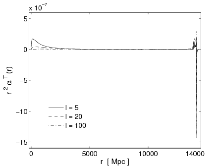
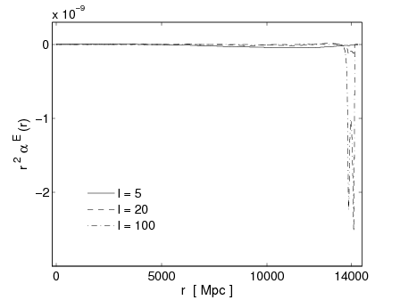
To be able to perform the steps outlined in the last section, we first have to precompute the necessary auxiliary data. This needs to be done only once for a given set of cosmological parameters. First, we obtained the transfer functions in momentum space from a modified version of the latest CAMB software package333Obtained from http://camb.info (Lewis et al. 2000). We then derived their equivalent expressions in real space using Eq. 6. Examples of temperature and polarization transfer functions as a function of conformal distance for several multipole moments are shown in 1.
As a next step, we calculate the covariance matrix of the gravitational potential on a fine grid with shells from the origin to the present time cosmic horizon (Eq. 7). As a start, we resolve the last scattering surface with uniform spacing using an increment of and chose a larger interval elsewhere (). This simple approach will be refined later. Using the derived quantities, it is now possible to generate and numerically solve the radial integral Eq. 5 to obtain simulated non–Gaussian CMB maps. However, significant improvement in the numerical evaluation of the integral is achievable by choosing both weights and quadrature points in an optimal way, as we will show in the following.
Keeping the multipole moment fixed for simplicity, we want to accurately compute the integral
| (10) |
This is done in a two step process: We first approximate Eq. 10 with a discrete sum over shells. Then, we try to obtain comparable accuracy with fewer shells introducing weights,
| (11) |
where the gravitational potential is evaluated at the nodes and weighted by the factors . Now, we can derive the expectation value of the quadratic error
| (12) |
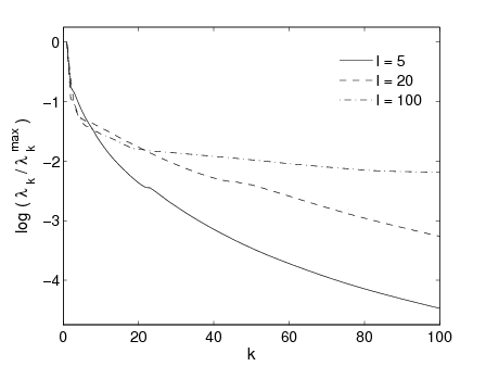
where we have introduced the eigenvalues and eigenvectors of the covariance matrix of the potential on the fine grid with elements. We show for several multipole moments in the left panel of 2. If the eigenvalues decrease sufficiently fast, the error is expected to be low already for a small number of quadrature points . This seems especially to be true on large angular scales. However, this finding is partially counterbalanced by the fact that the transfer functions are significantly different from zero at small radii for low multipole moments (late ISW effect, reionization), enforcing the inclusion of additional nodes.
Based on the expression for the expected quadratic error, it is straightforward to calculate optimal weights by satisfying the condition , which leads to a system of linear equations,
| (13) |
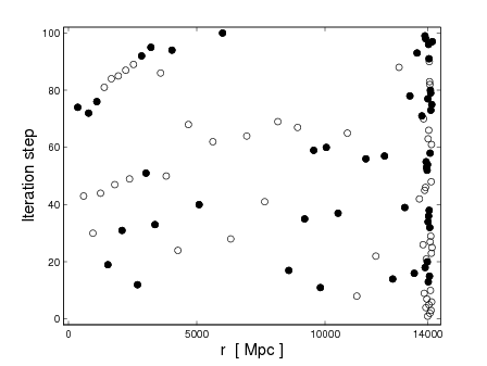
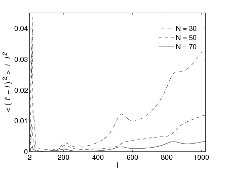
Even more important, Eq. 12 allows us to formulate a greedy algorithm to compute optimal quadrature points. We select a subset of nodes out of the fine radial grid with 400 elements iteratively, in each step including the point that most efficiently reduces the remaining error. To simultaneously optimize for temperature and polarization, we add the expectation values of the two errors with equal weights. We use the outcome of the procedure to tune the radii of the input grid with 400 elements. We choose a smaller spacing down to at the last scattering surface, where nodes were selected with the highest priority, and a larger step size up to at distances, where the quadrature points were classified as less important. Then, we repeated the optimization process a second time. In the right panel of 2, we visualize the first 100 iterations of the optimization scheme. We display the expectation value of the relative quadratic error for and quadrature points in 3. The raise in error towards the largest angular scales is caused by the increasing contribution from late ISW effect and reionization.

As a last step, we show how to reduce the memory consumption of the code. Whereas the potentials and can be co–added to the spherical harmonic coefficients of the CMB map and (Eq. 5) one shell after another, the radial correlation of forces one to generate it at all shells simultaneously, potentially requiring large amounts of memory. To circumvent this problem, we keep the random seeds that were used to draw the potential. By means of the seeds, we are able to easily regenerate the gravitational potential at any radii . Thus, we only store its real space representation at the radius that is currently added to the CMB map, substantially reducing the overall memory consumption of the algorithm.
Having optimized the simulation algorithm in this way, we generated realizations of temperature and polarization CMB maps. We chose a HEALPix resolution parameter of and a maximum multipole moment of . We used quadrature points for evaluation of Eq. 5, although we stress that this choice is conservative and it is possible to derive reasonable results with smaller values of .
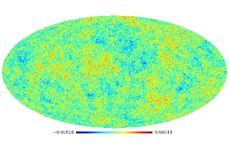
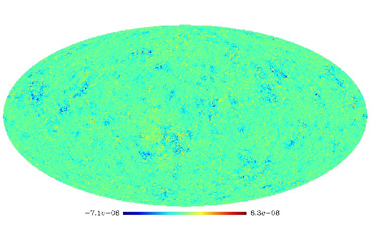
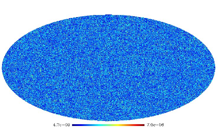
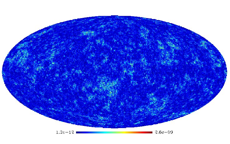
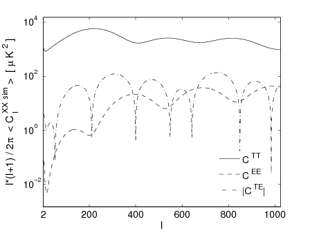
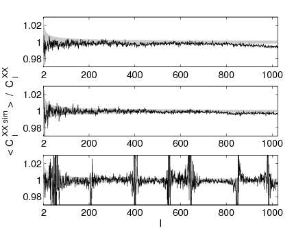
With these input parameters, we aim for sub–percentage accuracy of the final map over the entire range of multipole moments, guided by the intrinsic precision of the underlying transfer functions, running CAMB with RECFAST at standard accuracy. An example is displayed in 4, where we illustrate a realization of temperature and polarization maps of the linear and non–linear part of the CMB. We show the averaged power spectra of all simulations along with a comparison to the theoretical values in 5. A detailed comparison to the expected statistical fluctuations () reveals remaining slight systematic deviations for the TT and EE spectra at high at the level of less than 1% of the input power spectrum. If required this error could be further reduced by adding integration nodes. It takes about 20 minutes to generate a single map with the given resolution on a single Intel Xenon processor with a clock rate of 2.33 GHz, requiring only a modest amount of memory (). The most time consuming part is the evaluation of the spherical harmonic transforms necessary to compute the non–Gaussian potential.
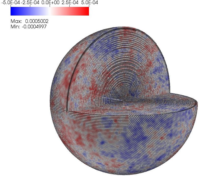
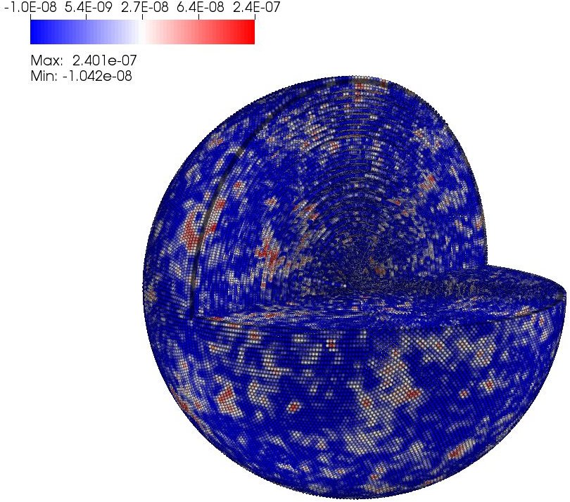
The algorithm described here generates valid realizations of primordial curvature perturbations in real space. This itself is an interesting quantity and can be used to e.g. test the performance of reconstruction techniques as we will show in the next section. We visualize the 3D gravitational potential and in 6; long–distance correlations on large scales are in evidence.
Our simulation algorithm is conceptually very similar to the method proposed in Liguori et al. (2007), where the authors generate the gravitational potential on 400 shells, requiring 800 spherical harmonic transforms to calculate a single non–Gaussian CMB map, and report a runtime of 3 hours for . By applying our optimized quadrature scheme, we have demonstrated that it is possible to reduce the number of transforms considerably, resulting in an increase of computational efficiency. Another, albeit more formal difference is the way the gravitational potential is generated. We use the real space covariance matrix to draw directly, whereas the authors of Liguori et al. (2007) compute the gravitational potential by performing an integral over uncorrelated random numbers weighted by ‘filter’ functions.
In Smith & Zaldarriaga (2006), where the authors focused on a perturbative reproduction of the correct bispectrum in the regime of weak non–Gaussianity, a runtime of about three minutes is reported to simulate one non–Gaussian CMB temperature map at an angular resolution of . Although slower by an order of magnitude, and tuned for local non–Gaussianity, the algorithm presented here is capable of simulating both temperature and polarization maps (i.e. three maps for the stokes parameter I, Q, and U) within the same framework and with nearly the same computational cost compared to temperature alone. Furthermore, as recently pointed out by Hanson et al. (2009), in the case of local non–Gaussianity an additional modification of the algorithm of Smith & Zaldarriaga (2006) is necessary to suppress the power spectrum of the non–Gaussian part of a simulated map, found to be artificially enhanced by several orders of magnitudes on large angular scales.
Notwithstanding the aforementioned higher computational costs, we regard our method as useful for the study of local non–Gaussianity, because the simulated maps are well suited to test any kind of estimator, e.g. based on Minkowsky functionals (Spergel et al. 2007; Hikage et al. 2008), or a wavelet analysis (Martínez-González et al. 2002; Mukherjee & Wang 2004). If a detection of nonzero is reported, it will be important to confirm the result with alternative statistical tools, as they are sensitive to different systematic effects.
In the following section, we apply the KSW estimator (Komatsu et al. 2005) to our set of simulated maps with known non–Gaussian contribution to test whether the input values for can be recovered.
4 Bispectrum Analysis
As we do not aim to describe the fast estimator in detail, we include a brief summary here and refer the reader to the extensive literature for further details and a comprehensive discussion (e.g. in Komatsu et al. 2005; Smith & Zaldarriaga 2006; Creminelli et al. 2007; Yadav et al. 2007).
To estimate the non–Gaussianity of a CMB map, one constructs the statistic out of a cubic combination of the data,
| (14) |
The radial integral runs over two filtered maps,
| (15) | ||||
| (16) |
that are constructed using the auxiliary functions
| (17) | ||||
| (18) |
and the inverse of the matrix containing the CMB power spectrum elements,
| (19) |
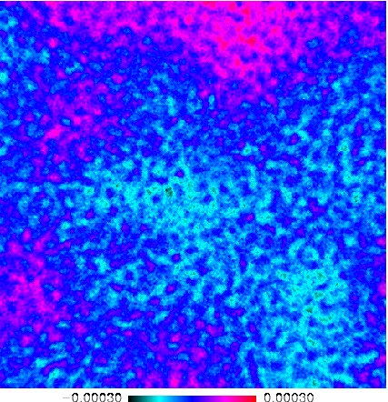
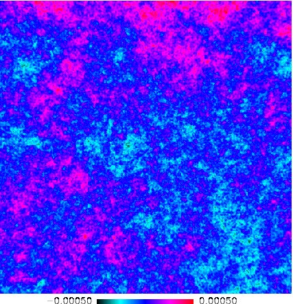
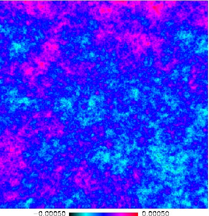
One of these maps, , is exactly the Wiener filter reconstruction of the underlying gravitational potential . With the simulation algorithm presented in Sect. 2, it is possible to compare the potential used to synthesize the map with its reconstruction directly. An example is shown in 7, where we depict the reconstruction of the potential around last scattering using only temperature, and using both, temperature and polarization information.
As the estimator is proportional to the non–Gaussianity parameter , we can calculate its expectation value by applying a suitable normalization,
| (20) |
where , when , 2, when or , and 1 otherwise. We further introduced the theoretical bispectrum for , which is defined as
| (21) |
where the prefactor is given by
| (22) |
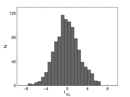
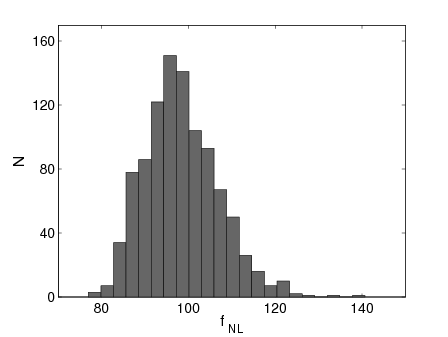
We used the equations above to implement the fast estimator for temperature and polarization. As our primary goal is to validate our simulation algorithm, we do not take into account possible instrumental effects, sky cut, or noise. To test our simulations, we generate two sets of 1000 CMB temperature and polarization maps with resolution parameter , and . We consider one sample of purely Gaussian realizations of the CMB sky (), and one non–Gaussian sample with a fiducial value of . We then run the fast estimator on the maps to compute an estimate of . We show the distribution of the derived values in 8. We find the input parameters to be recovered well, the means of the distributions are and for the Gaussian and non–Gaussian simulations, respectively. The estimated standard deviations are and , compared to the expected error predicted from a Fisher information matrix analysis of . We conclude that the algorithm outlined in Sect. 2 and implemented as described in Sect. 3 produces valid realizations of non–Gaussian CMB temperature and polarization maps.
5 Summary
In this paper, we introduced a new algorithm to simulate temperature and polarization CMB maps containing non–Gaussianity of arbitrary local type. In the proposed scheme, we generate spherical harmonic coefficients of the Gaussian potential as a function of conformal distance, taking into account the proper radial correlations. Then, the potential is transformed to pixel space to compute the associated non–Gaussian contribution. Finally, we make use of the real space representation of the transfer functions to perform the line of sight integral in order to calculate Gaussian and non–Gaussian contribution to the CMB maps.
We developed and applied a quadrature scheme that allows us to increase the numerical efficiency of the code. As a starting point, we derived an expression to quantitatively calculate the mean error introduced by replacing the radial integral by a finite sum. On that basis, we were able to choose both, nodes and weights for numerical quadrature in an optimal way. As a last step, we successfully reduced the memory consumption of the algorithm.
For WMAP5+BAO+SN cosmological parameters, we simulated 1000 realizations of non–Gaussian CMB temperature and polarization maps with resolution parameters and . To validate the algorithm, we applied the well studied and widely accepted fast cubic (bispectrum) estimator to the simulations. For both, a set of Gaussian and non–Gaussian realizations of CMB sky maps, the input parameters were consistently recovered. We make our simulations publicly available at http://planck.mpa-garching.mpg.de/cmb/fnl-simulations.
References
- Alishahiha et al. (2004) Alishahiha, M., Silverstein, E., & Tong, D. 2004, Phys. Rev. D, 70, 123505
- Bardeen et al. (1983) Bardeen, J. M., Steinhardt, P. J., & Turner, M. S. 1983, Phys. Rev. D, 28, 679
- Chen (2005) Chen, X. 2005, Phys. Rev. D, 72, 123518
- Creminelli et al. (2007) Creminelli, P., Senatore, L., & Zaldarriaga, M. 2007, Journal of Cosmology and Astro-Particle Physics, 3, 19
- Enqvist & Sloth (2002) Enqvist, K. & Sloth, M. S. 2002, Nucl. Phys., B626, 395
- Górski et al. (2005) Górski, K. M., Hivon, E., Banday, A. J., et al. 2005, ApJ, 622, 759
- Guth (1981) Guth, A. H. 1981, Phys. Rev. D, 23, 347
- Hanson et al. (2009) Hanson, D., Smith, K. M., Challinor, A., & Liguori, M. 2009, ArXiv e-prints
- Hikage et al. (2008) Hikage, C., Matsubara, T., Coles, P., et al. 2008, MNRAS, 389, 1439
- Khoury et al. (2001) Khoury, J., Ovrut, B. A., Steinhardt, P. J., & Turok, N. 2001, Phys. Rev. D, 64, 123522
- Komatsu et al. (2003) Komatsu, E., Kogut, A., Nolta, M. R., et al. 2003, ApJS, 148, 119
- Komatsu & Spergel (2001) Komatsu, E. & Spergel, D. N. 2001, Phys. Rev. D, 63, 063002
- Komatsu et al. (2005) Komatsu, E., Spergel, D. N., & Wandelt, B. D. 2005, ApJ, 634, 14
- Langlois et al. (2008) Langlois, D., Renaux-Petel, S., Steer, D. A., & Tanaka, T. 2008, Phys. Rev. D, 78, 063523
- Lehners & Steinhardt (2008) Lehners, J.-L. & Steinhardt, P. J. 2008, Phys. Rev. D, 77, 063533
- Lewis et al. (2000) Lewis, A., Challinor, A., & Lasenby, A. 2000, ApJ, 538, 473
- Liguori et al. (2003) Liguori, M., Matarrese, S., & Moscardini, L. 2003, ApJ, 597, 57
- Liguori et al. (2007) Liguori, M., Yadav, A., Hansen, F. K., et al. 2007, Phys. Rev. D, 76, 105016
- Lyth et al. (2003) Lyth, D. H., Ungarelli, C., & Wands, D. 2003, Phys. Rev. D, 67, 023503
- Martínez-González et al. (2002) Martínez-González, E., Gallegos, J. E., Argüeso, F., Cayón, L., & Sanz, J. L. 2002, MNRAS, 336, 22
- Moroi & Takahashi (2001) Moroi, T. & Takahashi, T. 2001, Phys. Lett., B522, 215
- Mukhanov et al. (1992) Mukhanov, V. F., Feldman, H. A., & Brandenberger, R. H. 1992, Phys. Rep., 215, 203
- Mukherjee & Wang (2004) Mukherjee, P. & Wang, Y. 2004, ApJ, 613, 51
- Senatore (2005) Senatore, L. 2005, Phys. Rev. D, 71, 043512
- Smith & Zaldarriaga (2006) Smith, K. M. & Zaldarriaga, M. 2006, ArXiv Astrophysics e-prints
- Spergel et al. (2007) Spergel, D. N., Bean, R., Doré, O., et al. 2007, ApJS, 170, 377
- Steinhardt & Turok (2002) Steinhardt, P. J. & Turok, N. 2002, Phys. Rev. D, 65, 126003
- Verde et al. (2000) Verde, L., Wang, L., Heavens, A. F., & Kamionkowski, M. 2000, MNRAS, 313, 141
- Yadav et al. (2007) Yadav, A. P. S., Komatsu, E., & Wandelt, B. D. 2007, ApJ, 664, 680