Quantitative and Conceptual Considerations for Extracting the Knudsen Number in Heavy Ion Collisions
Abstract
In this paper we examine the methodology for extracting the Knudsen number () and the ratio of shear viscosity to entropy density () developed by Drescher et al Drescher:2007cd . The final result for turns out to be quite sensitive to Glauber parameters, and particularly the parameter which controls the balance between and . We also explore how alternative formulations of the functional relation between the elliptic flow and Knudsen number () impacts the physics conclusions, based on Padé approximants. Finally, we extend the calculation to include a limiting minimum value on the mean free path proportional to the DeBroglie wavelength. These results emphasize the importance of clarifying the initial state used in different calculations, as well as the ambiguities inherent in using a transport approach in a strongly-coupled regime.
pacs:
25.75.DwI Introduction
The medium created in heavy ion collisions at the Relativistic Heavy Ion Collider (RHIC) defied expectations by showing a strong collective flow, characteristic of a perfect fluid Arsene:2004fa ; Adcox:2004mh ; Back:2004je ; Adams:2005dq . This behavior is particularly striking since even a modest amount of viscous damping, parametrized as the ratio of shear viscosity to the entropy density , is predicted to result in large deviations from ideal hydrodynamics Teaney:2003kp . Several methods, each subject to as-yet uncontrolled systematic uncertainties, have been developed to estimate the value of () from the experimental data on collective flow Lacey:2006bc ; Drescher:2007cd , fluctuations Gavin:2006xd , and heavy quark transport Adare:2006nq . A parallel effort in this direction has been the development of hydrodynamic codes in two and three dimensions with a properly causal and stable relativistic treatment of viscous effects to second order in the velocity gradients Song:2007ux ; Romatschke:2007mq ; Luzum:2008cw ; Molnar:2008xj ; Chaudhuri:2008sj . While recent work has resulted in a greatly improved understanding of the various formalisms used by these authors TECHQM , and direct comparison to experimental data has been made for a range of values in , there remains considerable debate regarding the sensitivity to initial conditions, equations of state, and precise freeze-out conditions.
These different approaches are in large part motivated by the conjecture Kovtun:2004de that there is a fundamental bound on the viscosity to entropy density ratio: . Intriguingly, all methods produce values for from the RHIC fluid that are within factors of 1-4 of the bound. This brings into sharp focus the need to understand in detail the utility and the limitations of each method. In this paper we concentrate on the approach of Drescher et al. Drescher:2007cd , which provides a useful framework for parameterizing departures from ideal hydrodynamic behavior in terms of the Knudsen number , where is the mean free path of particles or quasi-particles in the system and is a characteristic measure of the system size.
It has been realized since the earliest applications of hydrodynamics to nuclear collisions (see the first two footnotes of Ref. Belenkij:1956cd ) that the determination of is directly related to the viscosity of the fluid. For sufficiently small values of the hydrodynamic limit is reached, but larger values imply the presence of a non-trivial mean free path, leading to the damping of momentum anisotropies, and thus deviations from ideal fluid behavior. In Ref. Drescher:2007cd the Knudsen number is directly related to the elliptic flow scaled by the initial state eccentricity , thereby providing a convenient link between the experimental data and the transport properties of the medium.
II Methodology
In this section we review the previous extraction of the Knudsen number and the the ratio as formulated in Ref. Drescher:2007cd . In doing so, we demonstrate the sensitivity to various assumptions at different steps in the calculation. Following Bhalerao et al. Bhalerao:2005mm , Ref. Drescher:2007cd takes the characteristic size of the system as the scale of the strongest gradient in the initial matter configuration of the system, estimated by
| (1) |
This expression for is used to determine the Knudsen number, which in turn is assumed to describe deviations of the the elliptic flow parameter () scaled by the initial eccentricity from the corresponding ratio for ideal hydrodynamics via
| (2) |
where is a parameter estimated to be approximately 0.7 from varying the particle cross-section in a 3D transport code Chen:2005mr , or by comparison to a Monte Carlo solution of a two-dimensional Boltzmann equation Gombeaud:2007ub . The parametric dependence on in Eqn. 2 is not directly motivated by an underlying microscopic theory, but rather was proposed in Ref. Bhalerao:2005mm to have the correct limits in the two extremes of large and small . In the limit of large mean-free path (large ) , while in the small mean-free path (small ) limit approaches the limiting ideal fluid or hydrodynamic value with corrections linear in . If the functional form of Eqn. 2 was unique (to be discussed below), then it is clear that by combining the value of calculated using ideal hydrodynamics with an experimental measure of would permit a direct determination of (albeit with the embedded uncertainties of hydrodynamic calculations mentioned in the introduction). Even more appealing is the possibility developed in Ref. Drescher:2007cd of directly determining both and by fitting the experimental data on as a function of centrality.
The Knudsen number varies with centrality both directly via associated changes in and indirectly through changes in the particle number density :
| (3) |
where is the effective inter-particle cross-section. Please note that having well-defined values for , and implicitly assumes classical ballistic transport. The prescription for estimating from the experimental data comes from Ref. Bhalerao:2005mm
| (4) |
which relies on calculations (for example from Monte Carlo Glauber Alver:2008aq ) to determine the transverse area of the system and the assumption of Bjorken expansionBjorken:1982qr with as an appropriate proper time in a rapidity slice. The characteristic time over which the gradients develop was assumed in Ref. Bhalerao:2005mm to be where is the speed of sound from the equation of state, giving:
| (5) |
and thus (by Eqn. 3):
| (6) |
Note that with these assumptions the Knudsen number no longer requires knowledge of . One can then eliminate the Knudsen Number entirely and write Eqn. 2 in terms of these new quantities.
| (7) |
which indicates that fitting plots of the experimental values of as a function of another ‘experimental quantity can be used to determine ) and . This approach is then applied to PHOBOS measurements of in Cu+Cu and Au+Au collisions at GeV for unidentified hadrons at pseudo-rapidity as a function of the number of participating nucleons () Back:2004mh ; Alver:2006wh ; Alver:2008zza . We note here and below that the that appears in these equations is that for total particle (presumably parton) rapidity density, so that further (plausible) assumptions are required to express this in terms of the experimentally measured charged-particle pseudo-rapidity density .
III Details of the Input Parameters
In this section we describe the uncertainties associated with the determination of the eccentricity-scaled elliptic flow and the parton transverse areal density . Close examination finds that the PHOBOS data presented in Fig. 1 of Ref. Drescher:2007cd appears quite different from what is nominally the same data presented in Fig. 6 of Ref. Alver:2006wh . This is explained primarily by the fact that while the extraction of the Knudsen number is based on experimental data, the approach relies on various geometric quantities (e.g. the area , the eccentricity ) which are not measured directly, but which are only estimated for each centrality bin. Detailing the differences is instructive and points out systematic uncertainties that must be addressed before a fully quantitative estimate of can be made.
One significant source of uncertainty in all such calculations is the lack of knowledge about the initial distribution of energy and matter that is relevant for the calculation of the initial eccentricity and the overlap area . In Ref. Drescher:2007cd , two initial conditions are presented representing different assumptions about the initial state, one from a Monte Carlo Glauber (MCG) calculation and the other from a particular Color Glass Condensate (CGC) calculation Drescher:2006ca . For the MCG case the initial distribution of energy is defined by a combination of spatial coordinates of participating nucleons and binary collisions. The relative weights of the contributions follow the “two-component” model of Kharzeev and NardiKharzeev:2000ph :
| (8) |
with , the so-called “80:20” mixture. This nomenclature is potentially misleading: In central Au+Au collisions , which implies that the term contributes only 40% of the matter while contributes 60%. It is also notable that the chosen value of is not commonly used in the literature (e.g. Ref. Kharzeev:2000ph ) and the experimental data at mid-rapidity at all beam energies is best described by Back:2004dy .
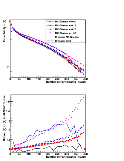
Fig. 1 shows a new calculation of the eccentricity values using a modified version of the PHOBOS MC code phobos_glauber_hepforge where we have incorporated the two-component model. Note that we use the standard nuclear parameters and no nucleon-nucleon hard core potential (). We calculate the eccentricity values from the Monte Carlo event-by-event by the following equation:
| (9) |
The notation will be used even for , i.e. when the weighting is not just for the participants. For comparisons with PHOBOS data, the second cumulant is used, since the event plane method is effectively a two particle correlation Alver:2008zza .
Fig. 1 shows the value of for Au+Au collisions as a function of for four values of = 0.0, 0.13, 0.20, and 1.00. The lower panel of Fig. 1 shows the ratio of each case relative to the case. Results from Ref. Drescher:2007cd for are also shown. We find that our results for are systematically larger than their results. This discrepancy has been traced to the fact that the analysis in Ref. Drescher:2007cd uses a non-standard form for Eqn. 8, with a weight of one (as opposed to ) for the term. This difference then gives a larger weighting for the spatial distribution of participants (i.e. lower value), though there is no mapping onto a different exact value given by Eqn. 8. We also show the eccentricity values for their Color Glass Condensate calculation for comparison, which interestingly track our case, i.e. follow the density of the binary collisions, except in the most central collisions.
We have also checked the eccentricity fluctuations for the different assumptions to see if this might offer an experimental method to discriminate between different values. The results show that the event-to-event fluctuations in eccentricity are the same for all cases within 3-6%. As one might expect, the fluctuations are somewhat smaller for the = 1.00 case, since there are a larger number of binary collisions to smooth out the fluctuations compared with participants. However, this difference is affected by the spatial correlations between binary collisions and might even be further modified with inclusion of a nucleon-nucleon hard core potential (i.e. a non-zero value of ).
In addition to the differences in eccentricities even for the case of identical values, there are a number of differences we have uncovered that we describe below.
-
•
The average overlap area is calculated using the following equation:
(10) corresponding to the area of the tilted ellipse. It should be noted that, in the literature, this equation appears in with various prefactors (e.g. Alver:2008zza , Bhalerao:2005mm , and Gombeaud:2007ub ). The prefactor gives a somewhat more intuitive result, as it yields the correct answer for the simple case of a disc with uniform density. This convention is utilized in the remainder of this paper. However, since the parton density is not uniform, it is possible that one should consider a smaller area (for example in a core/corona type picture).
In the extraction of the product from Eqn. 2, any multiplicative scaling of the vertical-axis quantity does not change the extracted results, but a multiplicative scaling of the horizontal-axis results in a linear change in . However, we later note that simple multiplicative scaling of these quantities cancels in the determination .
Finally, Ref. Drescher:2007cd does not calculate the overlap area in the tilted (i.e. fluctuating event-by-event) frame. This turns out to be a minor (1-2%) difference, since the cross term turns out to be relatively small compared to the other two moments.
-
•
The experiments do not measure the parton density at early times, but instead measure after freeze-out. The rapidity density is extracted from the measured by multiplying by a simple estimate of the Jacobian factor of 1.15. However, this factor depends on the particle mix and momentum spectra, which are not measured by PHOBOS over their full acceptance. In the calculations of Drescher et al., they have converted the to with a factor 1.25; however, in our calculations we have used the factor utilized by PHOBOS of 1.15Alver:2008zza . One can then convert from charged hadrons to all hadrons by assuming a multiplicative factor of 1.5. It should be noted that equating this hadron density to the parton density requires the additional assumption of local parton-hadron duality, with an exact factor of 1.0 scaling. Each of these factors enters as a linear scaling of the horizontal-axis quantity .
-
•
Ref. Drescher:2007cd calculates the average of the product (i.e. ) in the Monte Carlo approachm, for both CGC and Glauber. In contrast, since PHOBOS uses the measured and calculate for each centrality bin, they determine the product of averages (i.e. .). If one wants to use the average of the product, one cannot directly utilize the PHOBOS measured as a function of , since one no longer has a model of the correlated fluctuations between the two quantities. Instead one must use a parametrization based on the MCG calculation event-by-event. Throughout this paper, we calculate the average of the product. We have also checked in the MCG calculation that taking the product of the averages and find differences in the extracted fit parameters of order 20%.
In our calculations, even though and are calculated with different values, is always used to determine the charged particle multiplicity. This is because any case considered should have the correct particle multiplicity input (which is not described by significantly different values within the two-component model). Thus, one should think of varying as an arbitrary way of modifying the initial geometry while maintaining the correct multiplicity at a given centrality. If one were certain that the charged particle multiplicity constrains the geometry only around 0.13, then these other scenarios might be ruled out. It is also notable that for the Cu+Cu data, there is a disagreement between this parametrization of the charged particle multiplicity at mid-rapidity by approximately 10% in the most central events.
One final comment about the experimental uncertainties, and how they enter the fits. The PHOBOS data are presented graphically with vertical lines for the quadrature sum of statistical and systematic uncertainties at the 90% Confidence Level. Thus, they are scaled down by 1.6 to convert them into one standard deviation uncertainties for input to a fit. It is also not clear that the systematic uncertainties included here are uncorrelated point-to-point, which raises some issues about their inclusion in the standard fit. Were the correlations known, the modified fitting procedure developed in Adare:2008qa could be used to properly account for the correlations when determining the errors on the fitted parameters. We make an estimate of this possible systematic uncertainty correlation in the next section.
IV Extracting
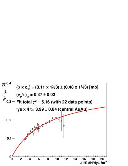
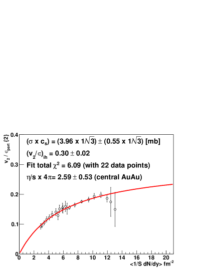
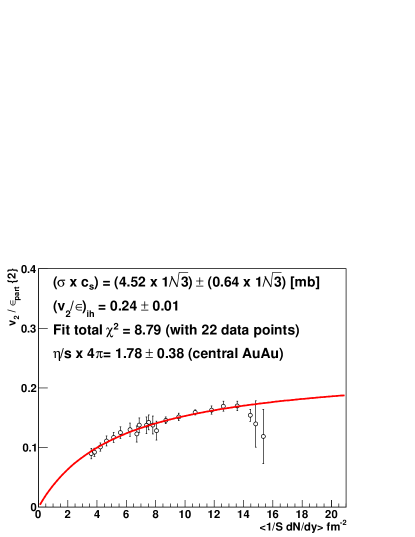
Fig. 2 shows the results from our calculations following the previously described prescription, using our MCG results with =0.00, =0.13, =1.00. Given the experimental data for as a function of transverse areal density, the fit procedure determines values and uncertainties for () and . Since only the product appears in the fit function, determination of the cross-section requires an explicit assumption for the sound speed. Taking for definiteness one obtains a cross-section value (in millibarns). The extracted values are shown in Fig. 2.
The extracted cross-section can be converted into a shear viscosity by using the results of a classical calculation Kox:76aa for massless particles at temperature interacting with isotropic cross-section
| (11) |
giving
| (12) |
In the second step the entropy was assumed to be given by , which follows from a definition of the number density using an ideal gas equation of state and the assumption of massless quanta with pressure (here only is the energy density). We note that there is already a 10% ambiguity here since it is common practice in astrophysics to compute the number densities directly from the Bose distribution functions KolbTurner , leading to 3.6 units of entropy per photon.
Taking MeV by assumption (another number with substantial uncertainty) and values for from the Monte Carlo Glauber, one can calculate for the most central Au+Au reactions at GeV. The resulting values are shown in each panel of Fig. 2, and are summarized with later results in Fig. 6. It is notable that the initial conditions with larger eccentricity (e.g. ) yield smaller values of . This is counterintuitive since a larger initial eccentricity should require a larger viscosity to reduce the down to the experimentally measured value. This result highlights that the extracted value of comes from the curvature of the data points as a function of centrality and the case indicates the largest degree of flattening (as seen in Fig. 2).
In principle each parameter has its own physics content, but it is interesting to check which parameters are necessary in order to extract directly. Since , one can directly write:
| (13) |
and quantities such as the speed of sound and the transverse overlap area do not explicitly appear. As a result, this form has the considerable advantage of explicitly demonstrating the parametric dependence of on the input parameters. Conversely, this simple expression holds only for the ’minimalist’ assumption for the -dependence given by Eqn. 2, and therefore imposes the need to investigate alternative parametrizations of this dependence, as discussed in the following section.
It is interesting to compare our results with those from Ref. Drescher:2007cd , who obtain = 2.38 using Monte Carlo Glauber = 0.20 (with the previously noted caveat regarding their non-standard definition) and = 1.38 using Color Glass Condensate initial conditions. Before comparing these values to our results, we note that there is a mistake in their calculation of in the CGC case. In the CGC case, in extracting the cross-section , they assume a speed of sound , but then use a density calculated with the input . As can be seen explicitly in our Eqn. 13, the speed of sound cancels out. Thus, the correct CGC value from their analysis is = 1.89. We also note that their quoted value of from reference Bhalerao:2005mm does not appear in that Letter, and must be converted for the difference in the prefactor, the use of optical Glauber versus Monte Carlo differences, and a missing Jacobian factor.
Taking these observations into account, we note that the values from our calculation for = 0.13 with for central Au+Au is similar to that from Ref. Drescher:2007cd for their = 0.20 with (despite the mismatch in exact eccentricities and other differences outlined above). Similarly, our calculation with = 1.00 gives , similar to Ref. Drescher:2007cd for the CGC case with (with the correction described above).
Here we re-visit the issue of the handling of the PHOBOS experimental systematic uncertainties. In the above we have considered them to be point-to-point uncorrelated. Since we do not know the full correlation matrix, we consider two cases to estimate of the systematic uncertainty on the extracted . If we allow the data points to move within the one standard deviation uncertainties in a correlated or anti-correlated manner (i.e. tilting the values around the mid-central point), we find that for the = 0.13 case, we obtain values of (moving the central points down and the peripheral points up) and (moving the central points up and the peripheral points down). We note that the total is very large in all cases in part because the statistical uncertainties are quite small and some part of the systematic uncertainty is likely uncorrelated. Thus, as an approximate estimate, the true fit uncertainty from the experimental uncertainties alone is most likely twice as large as that shown in Fig. 2. For the = 0.13 case, we then should state it as , instead of the previously quoted = .
V Other Parametrizations
It has already been noted that Eqn. 2 is not derived from any a priori theoretical expectation, but has been constructed to obey limiting functional forms at large and small . Given this, it is of interest whether an alternative functional form might fit the available data equally well and still obey the same two limits. A simple functional form (motivated by Padé approximants) is utilized here:
| (14) |
This equation obeys the large and small limits as the previous parametrization, if and . Of course one can obtain an infinite set of such equations by expanding the number of terms in the numerator and denominator. For this case, we constrain ourselves to the case where and . Fig. 3 shows the best fit where the additional parameter is allowed to vary (for the = 0.13 case). There is an approximately 25% decrease in the ideal hydrodynamic value , while the millibarns (assuming ) increases by about 25% relative to the previous value of , although with a larger uncertainty. This best fit corresponds to .
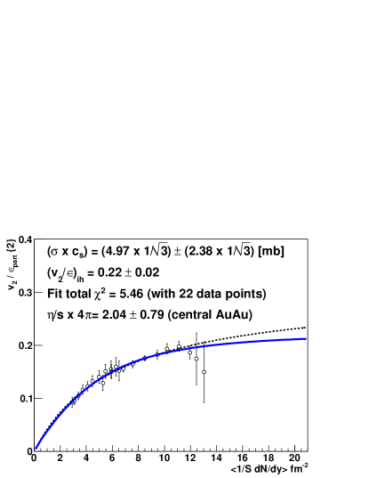
However, it turns out that the standard MINUIT fit has returned an incorrect uncertainty range because of a non-parabolic shape of the surface. The reason for this behavior is examined in Fig. 4, which shows all of the parameter fits with values within one standard deviation of the minimum, the total as a function of the extracted value, and the associated parameter values for and .
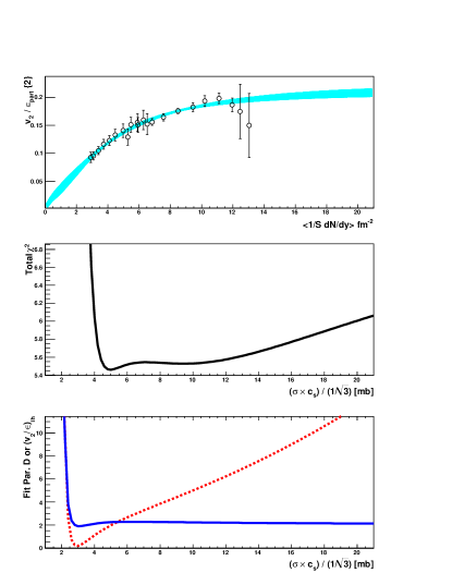
The presented as a function of () allows the determination of the uncertainty on at one-standard deviation to be millibarns. Almost any arbitrarily large value for the cross-section gives an equally good description of the experimental data with an almost identical value for and an increasing value of for larger values. Using Eqn. 12 to determine the corresponding values for we find an allowed range of from 2.55 all the way down 0.34 (well below the postulated bound).
These results indicate a certain fragility in the procedure outlined in Ref. Drescher:2007cd since a minimal modification of the parametrization amplifies the uncertainties in by an order of magnitude. It is therefore important to investigate if there are a priori theoretical restrictions on the functional dependence of on the Knudsen number. For example, are there theoretical arguments that might constrain . In a simple transport scenario with centrality independent cross-section , temperature , and speed of sound , one might question why the underlying dynamics would change significantly with centrality (i.e. ).
However, if obeying the two limits for is insufficient to determine the functional form, then one needs to make a proper theoretical argument about which types functional forms are truly relevant. There have been attempts to check the Knudsen number dependence with transport calculations and viscous hydrodynamic calculations Masui:2009pw , and these may lend support to the simple parametrization. However, if the parametrization is only tested in certain scenarios, then one has all the limitations of those particular scenarios and one cannot make more general conclusions.
VI Quantum Limits
One obvious feature of the above treatment is the lack of any explicit quantum bound on the value for . Clearly if such a bound exists, then the experimental values for cannot approach the ideal hydrodynamic limit, and it is unlikely that a transport formalism that allows violations of the bound would be applicable to the determination of in the vicinity of the bound. In this section we consider a modification of the formulation which explicitly incorporates the bound.
Following the original formulation of the bound Danielewicz:1984ww , we assume that the mean free path cannot be smaller than the DeBroglie wavelength of the particle. A simple prescription incorporating this limit is to modify the mean free path accordingly:
| (15) |
In the limit where , (the DeBroglie wavelength), while the limit gives the standard expression . Note that we are using natural units throughout.
In relating these values to we proceed as before
| (16) |
Taking (relevant for massless, non-interacting particles) the high density limit gives . Thus, there is a modest inconsistency (at the 40% level) between this implementation and the exact bound value. Note that it is possible to enforce the precise value of the bound by requiring , but in the interest of a simpler heuristic treatment we do not consider this additional modification. We highlight that even in the presence of quantum effects the Knudsen number itself can come arbitrarily close to zero, for example in a neutron star where any other scale in the problem.
The expression for as a function of is:
| (17) |
| (18) |
However, when using this expression into Eqn. 2 one needs to know the dependence of on before performing the fit. This dependence has been calculated with a Monte Carlo Glauber and then included in the fit to the experimental data.
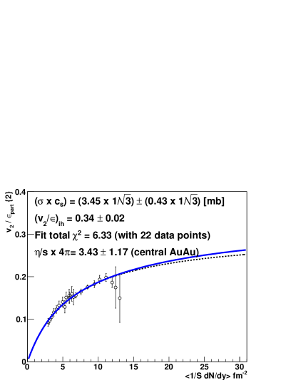
The resulting value of the fit is shown in Fig. 5. It gives a slightly smaller value of millibarns. This modest change is not surprising since the starting value without the correction is already a factor of 2.5 away from the quantum bound. For systems even closer to the bound, the impact would be much more significant. Note however that the extracted value of is almost larger than that extracted without incorporating the bound. This is not at all unexpected since one has re-interpreted the associated value with the asymptotic limit of the fit function.
VII Discussion
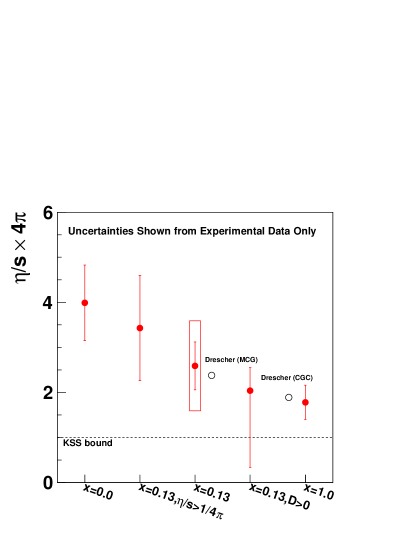
In this paper, we are not advocating the Knudsen number formalism as a rigorous method of extracting . Rather we are highlighting various issues with this methodology and note areas where systematic uncertainties are common to various methods that have been proposed for extracting . There are three main conclusions.
1. As has been previously observed, any method for extracting will be sensitive to the details of the initial conditions, and in particular the spatial distribution (and fluctuations) of the deposited energy density. This induces a strong sensitivity to the assumed ratio of binary collisions to participants in the Monte Carlo Glauber formalism since a modest centrality dependent change in the spatial distribution substantially changes the asymptotic behavior implied by the fit. This is particularly true because the experimental data does not have small enough uncertainties for central Au+Au events to determine whether an asymptotic limit has been reached. This is the main reason why choosing a different functional form for the Knudsen number parametrization allows almost any value for to be extracted, as demonstrated above.
In this paper we do not consider the Color Glass Condensate initial conditions in detail. However we note that there are at least two formulations that give significantly different results. These include calculations such as Ref. Lappi:2006xc which do not include fluctuations, and Ref. Drescher:2006ca which includes fluctuations and is the basis of the calculations by Drescher et al. shown in Fig. 1. The differences in CGC initial condition eccentricities are as large as the differences between Monte Carlo Glauber values, and thus this also needs to be addressed and reconciled.
These initial geometry uncertainties generally have a larger influence on this extraction method since a subtle difference in centrality dependence (i.e. curvature) can dramatically change the fit. Note that while Ref. Alver:2008zza finds the change in eccentricity from to for central Au+Au events to be 15% and thus considered small, we find that the change in the centrality dependence modifies the extracted value of by more than 50%.
These uncertainties certainly also influence other methods of extracting . We note that in the viscous hydrodynamic calculations in Ref. Luzum:2008cw , they consider two sets of initial conditions. In the Glauber case they utilize an optical model without fluctuations, and utilize the = 1.00 case. In contrast, Ref. Song:2007ux utilizes participants for initial conditions (i.e. ). In the case of constraints on from charm and bottom elliptic flow Adare:2006nq the extractions of will also depend on the initial conditions and the same scrutiny and propagation of uncertainties is needed. In Ref. Moore:2004tg they utilize an optical Glauber model without fluctuations and wounded nucleons (i.e. ), while in Ref. vanHees:2005wb they state that for impact parameter fm the eccentricity is .
These observations highlight the critical importance of a reproducible set of publicly available code for generating what are often simply referred to as “Glauber” initial conditions. All publications need a detailed specification of all relevant features of the Glauber calculation, including 1) the value, 2) Glauber parameters for the Woods-Saxon distribution, 3) any exclusion radius and re-weighting of the radius value, 4) any outer radius cut-off, 5) whether fluctuations in the reaction plane direction are included (as seen in Eqn. 9) 6) whether the result is not a Monte Carlo but instead an optical Glauber extraction. Many of the individual uncertainties related to these parameters have previously been considered minor (i.e. 20% or less).
2. Even if one accepts the assumptions of the formalism from Ref. Drescher:2007cd , there are significant uncertainties in the parameters characterizing the medium on time scales corresponding to the largest gradients, i.e. , and . Since these values vary as a function of both the space and time coordinates, one needs to specify the precise time and space interval over which the averaging is performed. It is also necessary to demonstate that such averaging of intermediate quantities is handled in a self-consistent fashion when deriving other averaged quantities (such as ). For example, the speed of sound is introduced into Eqn. 5 when estimating the characteristic time over which gradients develop. Absent a detailed simulation, the speed of sound in such an expression is an ill-determined average over times prior to the desired characteristic time. Nor is it obvious that this is same time-average assumed for other quantities such as , , , etc.
Moreover, there is also a potential inconsistency with the parameters used in studies up to this point. The temperature, parton density, speed of sound, and interaction cross-sections are not independent parameters. In fact at zero baryon density, the temperature determines all of the others. As an explicit example, a temperature of MeV is inconsistent with the speed of sound of when comparing with lattice QCD results at zero baryon chemical potential Karsch:2008fe . Also, temperature and parton density can be translated into and (energy density) via the QCD equation of state. While it seems reasonable that the temperature, density and speed of sound are approximately constant over the range of densities for Cu+Cu and Au+Au collisions at a single colliding energy (e.g. GeV) considered here, this is not expected to be true at asymptotically high densities. Even though there are no experimental data points at such densities, and one extracts and at the density corresponding to Au+Au central collisions, even small changes can systematically alter the centrality dependence, modifying the extracted value of , and thus . One must also consider the possibility of temperature dependent cross-sections in medium, something not addressed so far. Again, what are often dismissed as small centrality dependencies can modify the curvature of the data and have an unexpectedly large impact on .
We note that there has been a recent attempt to calibrate the simple analytic approach discussed here, utilizing viscous hydrodynamics calculations Masui:2009pw . These studies have already revealed an ambiguity in the value of and the equation of state. Additionally, any such calibration will have the same caveats and limitations of the existing viscous hydrodynamic calculations (with one such example being the absence of a hadronic phase after freeze-out).
3. In the formulation discussed in this paper, the extracted value of depends on whether or not a lower bound is explicitly introduced. Thus, if a lower bound on the viscosity does in fact exist, then extractions which do not incorporate it in their formalism will ultimately be unreliable. Conversely, approaches which enforce such a quantum bound on obviously cannot extract values below the bound. Thus one could never falsify the existence of such a bound. This is in contrast to full viscous hydrodynamic calculations and comparisons which do not rely on microscopic modeling of transport phenomena.
This raises the question at to whether the calculational framework discussed in Drescher et al., and this work, is valid in the strong-coupling limit, i.e. at . A standard Boltzmann transport calculation is the opposite limit from hydrodynamic calculation, which assume a continuum hypothesis. The theory community has explored both approaches with great benefit, and in both cases one can attempt to push the models past their nominal domains of applicability. If the viscous corrections to the ideal hydrodynamics are too large, then they violate the gradient expansion made in the small limit. In the Boltzmann transport approach (e.g. a parton cascade), the quasi-particle widths become of same order as the masses when the mean free paths are comparable to the DeBroglie wavelengths (i.e. ) LindenLevy:2007gd . As an example, if one ignored multi-particle quantum effects in a gas of cold atoms near the BEC transition that would have a dramatic impact on the physics picture. Thus, in this case, it is not clear how to determine the systematic uncertainties and overall physical picture.
VIII Summary
The formalism for relating to the Knudsen number has attracted much recent attention since it offers a tantalizing possibility of extracting transport properties almost directly from experimental data. However, several important issues need to be addressed consistently before one can consider this approach to produce anything more than order-of-magnitude estimates. The linearity of with , , and even makes a serious evaluation of their uncertainties of utmost important. One must also consider the fact that is a function of temperature due to the QCD equation of state itself. The final result for is quite sensitive to Monte Carlo Glauber parameters, and particularly the parameter which controls the balance between and . Finally, implementing a lower bound to , for instance as we have presented in this work, has a substantial effect on the extracted value, particularly since previous calculations find values so close to the bound already.
Acknowledgements.
We gratefully acknowledge useful discussions with Adrian Dmitru, Jean-Yves Ollitrault, Paul Romatschke, and Paul Stankus. JLN acknowledges support from the United States Department of Energy Division of Nuclear Physics grant DE-FG02-00ER41152. PAS is supported by U.S. Department of Energy grant DE-AC02-98CH10886. WAZ is supported by U.S. Department of Energy grant DE-FG02-86ER40281.References
- (1) H.-J. Drescher, A. Dumitru, C. Gombeaud, and J.-Y. Ollitrault, Phys. Rev. C76, 024905 (2007), 0704.3553.
- (2) BRAHMS, I. Arsene et al., Nucl. Phys. A757, 1 (2005), nucl-ex/0410020.
- (3) PHENIX, K. Adcox et al., Nucl. Phys. A757, 184 (2005), nucl-ex/0410003.
- (4) B. B. Back et al., Nucl. Phys. A757, 28 (2005), nucl-ex/0410022.
- (5) STAR, J. Adams et al., Nucl. Phys. A757, 102 (2005), nucl-ex/0501009.
- (6) D. Teaney, Phys. Rev. C68, 034913 (2003), nucl-th/0301099.
- (7) R. A. Lacey et al., Phys. Rev. Lett. 98, 092301 (2007), nucl-ex/0609025.
- (8) S. Gavin and M. Abdel-Aziz, Phys. Rev. Lett. 97, 162302 (2006), nucl-th/0606061.
- (9) PHENIX, A. Adare et al., Phys. Rev. Lett. 98, 172301 (2007), nucl-ex/0611018.
- (10) H. Song and U. W. Heinz, Phys. Rev. C77, 064901 (2008), 0712.3715.
- (11) P. Romatschke and U. Romatschke, Phys. Rev. Lett. 99, 172301 (2007), 0706.1522.
- (12) M. Luzum and P. Romatschke, (2008), 0804.4015.
- (13) D. Molnar and P. Huovinen, J. Phys. G35, 104125 (2008), 0806.1367.
- (14) A. K. Chaudhuri, (2008), 0801.3180.
- (15) https://wiki.bnl.gov/TECHQM/index.php/Bulk_Evolution.
- (16) P. Kovtun, D. T. Son, and A. O. Starinets, Phys. Rev. Lett. 94, 111601 (2005), hep-th/0405231.
- (17) S. Z. Belenkij and L. D. Landau, Nuovo Cim. Suppl. 3S10, 15 (1956).
- (18) R. S. Bhalerao, J.-P. Blaizot, N. Borghini, and J.-Y. Ollitrault, Phys. Lett. B627, 49 (2005), nucl-th/0508009.
- (19) L.-W. Chen and C. M. Ko, Phys. Lett. B634, 205 (2006), nucl-th/0505044.
- (20) C. Gombeaud and J.-Y. Ollitrault, Phys. Rev. C77, 054904 (2008), nucl-th/0702075.
- (21) B. Alver, M. Baker, C. Loizides, and P. Steinberg, (2008), 0805.4411.
- (22) J. D. Bjorken, Phys. Rev. D27, 140 (1983).
- (23) PHOBOS, B. B. Back et al., Phys. Rev. C72, 051901 (2005), nucl-ex/0407012.
- (24) PHOBOS, B. Alver et al., Phys. Rev. Lett. 98, 242302 (2007), nucl-ex/0610037.
- (25) B. Alver et al., Phys. Rev. C77, 014906 (2008), 0711.3724.
- (26) H. J. Drescher and Y. Nara, Phys. Rev. C75, 034905 (2007), nucl-th/0611017.
- (27) D. Kharzeev and M. Nardi, Phys. Lett. B507, 121 (2001), nucl-th/0012025.
- (28) PHOBOS, B. B. Back et al., Phys. Rev. C70, 021902 (2004), nucl-ex/0405027.
- (29) http://projects.hepforge.org/tglaubermc/.
- (30) PHENIX, A. Adare et al., Phys. Rev. Lett. 101, 232301 (2008), 0801.4020.
- (31) A. J. Kox, S. R. de Groot, and W. A. van Leeuwen, Physica A 84, 155 (1976).
- (32) E. W. Kolb and M. S. Turner, The Early Universe (Addison-Wesley, 1990).
- (33) H. Masui, J.-Y. Ollitrault, R. Snellings, and A. Tang, (2009), 0908.0403.
- (34) P. Danielewicz and M. Gyulassy, Phys. Rev. D31, 53 (1985).
- (35) T. Lappi and R. Venugopalan, Phys. Rev. C74, 054905 (2006), nucl-th/0609021.
- (36) G. D. Moore and D. Teaney, Phys. Rev. C71, 064904 (2005), hep-ph/0412346.
- (37) H. van Hees, V. Greco, and R. Rapp, Phys. Rev. C73, 034913 (2006), nucl-th/0508055.
- (38) RBC, F. Karsch, J. Phys. G35, 104096 (2008), 0804.4148.
- (39) L. A. Linden Levy, J. L. Nagle, C. Rosen, and P. Steinberg, Phys. Rev. C78, 044905 (2008), 0709.3105.