Statistical Topology via Morse Theory Persistence and Nonparametric Estimation

Peter Bubenik Department of Mathematics, Cleveland State University, Cleveland, Ohio 44115-2214 p.bubenik@csuohio.edu Gunnar Carlson Department of Mathematics, Stanford University, Stanford, California 94305 gunnar@math.stanford.edu Peter T. Kim Department of Mathematics and Statistics, University of Guelph, Guelph, Ontario N1G 2W1, Canada pkim@uoguelph.ca  and  Zhi–Ming Luo Department of Statistics, Keimyung University, Dalseo-Gu, Daegu, 704-701, Korea zluo@uoguelph.ca
Abstract.

In this paper we examine the use of topological methods for multivariate statistics. Using persistent homology from computational algebraic topology, a random sample is used to construct estimators of persistent homology. This estimation procedure can then be evaluated using the bottleneck distance between the estimated persistent homology and the true persistent homology. The connection to statistics comes from the fact that when viewed as a nonparametric regression problem, the bottleneck distance is bounded by the sup-norm loss. Consequently, a sharp asymptotic minimax bound is determined under the sup–norm risk over Hölder classes of functions for the nonparametric regression problem on manifolds. This provides good convergence properties for the persistent homology estimator in terms of the expected bottleneck distance.

Key words and phrases:
Bottleneck distance, critical values, geometric statistics, minimax, nonparametric regression, persistent homology, Plex, Riemannian manifold, sublevel sets.
2000 Mathematics Subject Classification:
Primary 62C10, 62G08; Secondary 41A15, 55N99, 58J90
Support for the second author was partially funded by DARPA, ONR, Air Force Office of Scientific Research, and NSF.
Support for the third author was partially funded by NSERC grant DG 46204.

1. Introduction

Quantitative scientists of diverse backgrounds are being asked to apply the techniques of their specialty to data which is greater in both size and complexity than that which has been studied previously. Massive, multivariate data sets, for which traditional linear methods are inadequate, pose challenges in representation, visualization, interpretation and analysis. A common finding is that these massive multivariate data sets require the development of new statistical methodology and that these advances are dependent on increasing technical sophistication. Two such data-analytic techniques that have recently come to the fore are computational algebraic topology and geometric statistics.

Commonly, one starts with data obtained from some induced geometric structure, such as a curved submanifold of a numerical space, or, a singular algebraic variety. The observed data is obtained as a random sample from this space, and the objective is to statistically recover features of the underlying space.

In computational algebraic topology, one attempts to recover qualitative global features of the underlying data, such as connectedness, or the number of holes, or the existence of obstructions to certain constructions, based upon the random sample. In other words, one hopes to recover the underlying topology. An advantage of topology is that it is stable under deformations and thus can potentially lead to robust statistical procedures. A combinatorial construction such as the alpha complex or the Čech complex, see for example [33], converts the data into an object for which it is possible to compute the topology. However, it is quickly apparent that such a construction and its calculated topology depend on the scale at which one considers the data. A multi–scale solution to this problem is the technique of persistent homology. It quantifies the persistence of topological features as the scale changes. Persistent homology is useful for visualization, feature detection and object recognition. Applications of persistent topology include protein structure analysis [30], gene expression [11], and sensor networks [8]. In a recent application to brain image data, a demonstration of persistent topology in discriminating between two populations is exhibited [5].

In geometric statistics one uses the underlying Riemannian structure to recover quantitative information concerning the underlying probability distribution and functionals thereof. The idea is to extend statistical estimation techniques to functions over Riemannian manifolds, utilizing the Riemannian structure. One then considers the magnitude of the statistical accuracy of these estimators. Considerable progress has been achieved in terms of optimal estimation [14, 12, 16, 26, 27, 19, 17]. Other related works include [28, 29, 23, 1, 3]. There is also a growing interest in function estimation over manifolds in the learning theory literature [7, 31, 2]; see also the references cited therein.

Although computational algebraic topology and geometric statistics appear dissimilar and seem to have different objectives, it has recently been noticed that they share a commonality through statistical sampling. In particular, a pathway between them can be established by using elements of Morse theory. This is achieved through the fact that persistent homology can be applied to Morse functions and comparisons between two Morse functions can be assessed by a metric called the bottleneck distance. Furthermore, the bottleneck distance is bounded by the sup–norm distance between the two Morse functions on some underlying manifold. This framework thus provides just enough structure for a statistical interpretation. Indeed, consider a nonparametric regression problem on some manifold. Given data in this framework one can construct a nonparametric regression function estimator such that the persistent homology associated with this estimated regression function is an estimator for the persistent homology of the true regression function, as assessed by the bottleneck distance. Since this will be bounded by the sup-norm loss, by providing a sharp sup–norm minimax estimator of the regression function, we can effectively bound the expected bottleneck distance between the estimated persistent homology and the true persistent homology. Consequently, by showing consistency in the sup-norm risk, we can effectively show consistency in the bottleneck risk for persistent homology which is what we will demonstrate. Let us again emphasize that the pathway that allows us to connect computational algebraic topology with geometric statistics is Morse theory. This is very intriguing in that a pathway between the traditional subjects of geometry and topology is also Morse theory.

We now summarize this paper. In Section 2 we will lay down the topological preliminaries needed to state our main results. In Section 3, we go over the preliminaries needed for nonparametric regression on a Riemannian manifold. Section 4 states the main results where sharp sup-norm minimax bounds consisting of constant and rate, and sharp sup-norm estimators are presented. The connection to bounding the persistent homology estimators thus ensues. Following this in Section 5, a brief discussion of the implementation is given. Proofs to the main results are collected in Section 6. An Appendix that contains some technical material is included for completeness.

2. Topological Preliminaries

Let us assume that 𝕄𝕄\mathbb{M} is a dlimit-from𝑑d-dimensional compact Riemannian manifold and suppose f:𝕄:𝑓𝕄f:\mathbb{M}\to\mathbb{R} is some smooth function. Consider the sublevel set, or, lower excursion set,

(2.1) 𝕄fr:={x𝕄|f(x)r}=f1((,r]).assignsubscript𝕄𝑓𝑟conditional-set𝑥𝕄𝑓𝑥𝑟superscript𝑓1𝑟\mathbb{M}_{f\leq r}:=\{x\in\mathbb{M}\ |\ f(x)\leq r\}=f^{-1}((-\infty,r]).

It is of interest to note that for certain classes of smooth functions, the topology of 𝕄𝕄\mathbb{M} can be approached by studying the geometry of the function.

To be more precise, for some smooth f:𝕄:𝑓𝕄f:\mathbb{M}\to\mathbb{R}, consider a point p𝕄𝑝𝕄p\in\mathbb{M} where in local coordinates the derivatives, f/xj𝑓subscript𝑥𝑗\partial f/\partial x_{j} vanishes. Then that point is called a critical point, and the evaluation f(p)𝑓𝑝f(p) is called a critical value. A critical point p𝕄𝑝𝕄p\in\mathbb{M} is called non-degenerate if the Hessian (2f/ij)superscript2𝑓subscript𝑖subscript𝑗(\partial^{2}f/\partial_{i}\partial_{j}) is nonsingular. Such functions are called Morse functions. Later we will see that differentiability is not needed when approached homologically.

The geometry of Morse functions can completely characterize the homotopy type of 𝕄𝕄\mathbb{M} by the way in which topological characteristics of sublevel sets (2.1) change at critical points. Indeed classical Morse theory tells us that the homotopy type of (2.1) is characterized by attaching a cell whose dimension is determined by the number of negative eigenvalues of the Hessian at a critical point to the boundary of the set (2.1) at the critical point. This indeed is a pathway that connects geometry with topology, and one in which we shall also use to bridge statistics. Some background material in topology and Morse theory is provided in Appendices A and B.

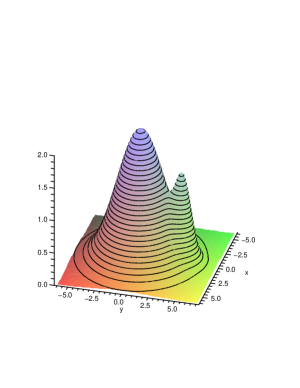
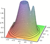
As motivation let us consider a real valued function f𝑓f that is a mixture of two bump functions on the disk of radius 101010 in 2superscript2\mathbb{R}^{2}, see Figure 2.1.

Refer to caption
Figure 2.1. A mixture of two bump functions and various contours below which are the sublevel sets.

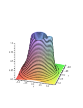
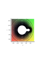
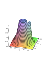
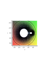
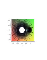
In this example, the maximum of f𝑓f equals 222, so 𝕄f2=𝕄subscript𝕄𝑓2𝕄\mathbb{M}_{f\leq 2}=\mathbb{M}. This sublevel set is the disk and therefore has no interesting topology since the disk is contractible. In contrast, consider the sublevel sets when r=1𝑟1r=1, 1.21.21.2, and 1.51.51.5 (see Figures 2.2, 2.3 and 2.4).

Refer to caption
Refer to caption
Figure 2.2. The sublevel set at r=1𝑟1r=1 has one hole.
Refer to caption
Refer to caption
Figure 2.3. The sublevel set at r=1.2𝑟1.2r=1.2 has two holes.
Refer to caption
Refer to caption
Figure 2.4. The sublevel set at r=1.5𝑟1.5r=1.5 has one hole.

In these cases, the sublevel sets 𝕄frsubscript𝕄𝑓𝑟\mathbb{M}_{f\leq r} have non-trivial topology, namely one, two and one hole(s) respectively, each of whose boundaries is one-dimensional. This topology is detected algebraically by the first integral homology group H1(𝕄fr)subscript𝐻1subscript𝕄𝑓𝑟H_{1}(\mathbb{M}_{f\leq r}) which will be referred to as the homology of degree 111 at level r𝑟r. This group enumerates the topologically distinct cycles in the sublevel set. In the first and third cases, for each integer z𝑧z\in\mathbb{Z}, there is a cycle which wraps around the hole z𝑧z times. We have H1(𝕄fr)=subscript𝐻1subscript𝕄𝑓𝑟H_{1}(\mathbb{M}_{f\leq r})=\mathbb{Z}. In the second case, we have two generating non-trivial cycles and so H1(𝕄fr)=subscript𝐻1subscript𝕄𝑓𝑟direct-sumH_{1}(\mathbb{M}_{f\leq r})=\mathbb{Z}\oplus\mathbb{Z}. For a review of homology the reader can consult Appendix A for related discussions.

2.1. Persistent topology

A computational procedure for determining how the homology persists as the level r𝑟r changes is provided in [10, 33]. In the above example there are two persistent homology classes (defined below). One class is born when r=1.1𝑟1.1r=1.1, the first sublevel set that has two holes, and dies at r=1.4𝑟1.4r=1.4 the first sublevel set for which the second hole disappears. The other class is born at r=0𝑟0r=0 and persists until r=2𝑟2r=2. Thus the persistent homology can be completely described by the two ordered pairs {(1.1,1.4),(0,2)}1.11.402\{(1.1,1.4),(0,2)\}. This is called the reduced persistence diagram (defined below) of f𝑓f, denoted 𝒟¯(f)¯𝒟𝑓\bar{\mathcal{D}}(f). For a persistent homology class described by (a,b)𝑎𝑏(a,b), call ba𝑏𝑎b-a its lifespan. From the point of view of an experimentalist, a long-lived persistent homology is evidence of a significant feature in the data, while a short-lived one is likely to be an artifact.

We now give some precise definitions.

Definition 2.1.

Let k𝑘k be a nonnegative integer. Given f:𝕄:𝑓𝕄f:\mathbb{M}\to\mathbb{R} and ab𝑎𝑏a\leq b\in\mathbb{R} the inclusion of sublevel sets iab:𝕄fa𝕄fb:superscriptsubscript𝑖𝑎𝑏subscript𝕄𝑓𝑎subscript𝕄𝑓𝑏i_{a}^{b}:\mathbb{M}_{f\leq a}\hookrightarrow\mathbb{M}_{f\leq b} induces a map on homology

Hk(iab):Hk(𝕄fa)Hk(𝕄fb).:subscript𝐻𝑘superscriptsubscript𝑖𝑎𝑏subscript𝐻𝑘subscript𝕄𝑓𝑎subscript𝐻𝑘subscript𝕄𝑓𝑏H_{k}(i_{a}^{b}):H_{k}(\mathbb{M}_{f\leq a})\to H_{k}(\mathbb{M}_{f\leq b}).

The image of Hk(iab)subscript𝐻𝑘superscriptsubscript𝑖𝑎𝑏H_{k}(i_{a}^{b}) is the persistent homology group from a𝑎a to b𝑏b. Let βabsuperscriptsubscript𝛽𝑎𝑏\beta_{a}^{b} be its dimension. This counts the independent homology classes which are born by time a𝑎a and die after time b𝑏b.

Call a real number a𝑎a a homological critical value of f𝑓f if for all sufficiently small ϵ>0italic-ϵ0\epsilon>0 the map Hk(iaϵa+ϵ)subscript𝐻𝑘superscriptsubscript𝑖𝑎italic-ϵ𝑎italic-ϵH_{k}(i_{a-\epsilon}^{a+\epsilon}) is not an isomorphism. Call f𝑓f tame if it has finitely many homological critical values, and for each a𝑎a\in\mathbb{R}, Hk(𝕄fa)subscript𝐻𝑘subscript𝕄𝑓𝑎H_{k}(\mathbb{M}_{f\leq a}) is finite dimensional. In particular, any Morse function on a compact manifold is tame.

Assume that f𝑓f is tame. Choose ϵitalic-ϵ\epsilon smaller than the distance between any two homological critical values. For each pair of homological critical values a<b𝑎𝑏a<b, we define their multiplicity μabsuperscriptsubscript𝜇𝑎𝑏\mu_{a}^{b} which we interpret as the number of independent homology classes that are born at a𝑎a and die at b𝑏b. We count the homology classes born by time a+ϵ𝑎italic-ϵa+\epsilon that die after time bϵ𝑏italic-ϵb-\epsilon. Among these subtract those born by aϵ𝑎italic-ϵa-\epsilon and subtract those that die after b+ϵ𝑏italic-ϵb+\epsilon. This double counts those born by aϵ𝑎italic-ϵa-\epsilon that die after b+ϵ𝑏italic-ϵb+\epsilon, so we add them back. That is,

μab=βa+ϵbϵβaϵbϵβa+ϵb+ϵ+βaϵb+ϵ.superscriptsubscript𝜇𝑎𝑏superscriptsubscript𝛽𝑎italic-ϵ𝑏italic-ϵsuperscriptsubscript𝛽𝑎italic-ϵ𝑏italic-ϵsuperscriptsubscript𝛽𝑎italic-ϵ𝑏italic-ϵsuperscriptsubscript𝛽𝑎italic-ϵ𝑏italic-ϵ\mu_{a}^{b}=\beta_{a+\epsilon}^{b-\epsilon}-\beta_{a-\epsilon}^{b-\epsilon}-\beta_{a+\epsilon}^{b+\epsilon}+\beta_{a-\epsilon}^{b+\epsilon}.

The persistent homology of f𝑓f may be encoded as follows. The reduced persistence diagram of f𝑓f, 𝒟¯(f)¯𝒟𝑓\bar{\mathcal{D}}(f), is the multiset of pairs (a,b)𝑎𝑏(a,b) together with their multiplicities μabsuperscriptsubscript𝜇𝑎𝑏\mu_{a}^{b}. We call this a diagram since it is convenient to plot these points on the plane. We will see that it is useful to add homology classes which are born and die at the same time. Let the persistence diagram of f𝑓f, 𝒟(f)𝒟𝑓\mathcal{D}(f), be given by the union of 𝒟¯(f)¯𝒟𝑓\bar{\mathcal{D}}(f) and {(a,a)}asubscript𝑎𝑎𝑎\{(a,a)\}_{a\in\mathbb{R}} where each (a,a)𝑎𝑎(a,a) has infinite multiplicity.

2.2. Bottleneck distance

Cohen–Steiner, Edelsbrunner and Harer [6] introduced the following metric on the space of persistence diagrams. This metric is called the bottleneck distance and it bounds the Hausdorff distance. It is given by

(2.2) dB(𝒟(f),𝒟(g))=infγsupp𝒟(f)pγ(p),subscript𝑑𝐵𝒟𝑓𝒟𝑔subscriptinfimum𝛾subscriptsupremum𝑝𝒟𝑓subscriptdelimited-∥∥𝑝𝛾𝑝d_{B}(\mathcal{D}(f),\mathcal{D}(g))=\inf_{\gamma}\sup_{p\in\mathcal{D}(f)}\lVert p-\gamma(p)\rVert_{\infty},

where the infimum is taken over all bijections γ:𝒟(f)𝒟(g):𝛾𝒟𝑓𝒟𝑔\gamma:\mathcal{D}(f)\to\mathcal{D}(g) and \|\cdot\|_{\infty} denotes supremum–norm over sets.

For example, let f𝑓f be the function considered at the start of this section. Let g𝑔g be a unimodal, radially-symmetric function on the same domain with maximum 2.22.22.2 at the origin and minimum 00. We showed that 𝒟¯(f)={(1.1,1.4),(0,2)}¯𝒟𝑓1.11.402\bar{\mathcal{D}}(f)=\{(1.1,1.4),(0,2)\}. Similarly, 𝒟¯(g)=(0,2.2)¯𝒟𝑔02.2\bar{\mathcal{D}}(g)=(0,2.2). The bottleneck distance is achieved by the bijection γ𝛾\gamma which maps (0,2)02(0,2) to (0,2.2)02.2(0,2.2) and (1.1,1.4)1.11.4(1.1,1.4) to (1.25,1.25)1.251.25(1.25,1.25) and is the identity on all ‘diagonal’ points (a,a)𝑎𝑎(a,a). Since the diagonal points have infinite multiplicity this is a bijection. Thus, dB(𝒟(f),𝒟(g))=0.2subscript𝑑𝐵𝒟𝑓𝒟𝑔0.2d_{B}(\mathcal{D}(f),\mathcal{D}(g))=0.2.

In [6], the following result is proven:

(2.3) dB(𝒟(f),𝒟(g))fgsubscript𝑑𝐵𝒟𝑓𝒟𝑔subscriptdelimited-∥∥𝑓𝑔d_{B}(\mathcal{D}(f),\mathcal{D}(g))\leq\lVert f-g\rVert_{\infty}

where f,g:𝕄:𝑓𝑔𝕄f,g:\mathbb{M}\to\mathbb{R} are tame functions and \|\cdot\|_{\infty} denotes sup–norm over functions.

2.3. Connection to Statistics

It is apparent that most articles on persistent topology do not as of yet incorporate statistical foundations although they do observe them heuristically. The approach in [25] combines topology and statistics and calculates how much data is needed to guarantee recovery of the underlying topology of the manifold. A drawback of that technique is that it supposes that the size of the smallest features of the data is known a priori. To date the most comprehensive parametric statistical approach is contained in [4]. In this paper, the unknown probability distribution is assumed to belong to a parametric family of distributions. The data is then used to estimate the level so as to recover the persistent topology of the underlying distribution.

As far as we are aware no statistical foundation for the nonparametric case has been formulated although [6] provide the topological machinery for making a concrete statistical connection. In particular, persistent homology of a function is encoded in its reduced persistence diagram. A metric on the space of persistence diagrams between two functions is available which bounds the Hausdorff distance and this in turn is bounded by the sup–norm distance between the two functions. Thus by viewing one function as the parameter, while the other is viewed as its estimator, the asymptotic sup–norm risk bounds the expected Hausdorff distance thus making a formal nonparametric statistical connection. This in turn lays down a framework for topologically classifying clusters in high dimensions.

3. Nonparametric regression on manifolds

Consider the following nonparametric regression problem

(3.1) y=f(x)+ε,x𝕄,formulae-sequence𝑦𝑓𝑥𝜀𝑥𝕄y=f(x)+\varepsilon,\ \ x\in\mathbb{M},

where 𝕄𝕄\mathbb{M} is a dlimit-from𝑑d-dimensional compact Riemannian manifold, f:𝕄:𝑓𝕄f:\mathbb{M}\to\mathbb{R} is the regression function and ε𝜀\varepsilon is a normal random variable with mean zero and variance σ2>0superscript𝜎20\sigma^{2}>0.

For a given sample (y1,x1),,(yn,xn)subscript𝑦1subscript𝑥1subscript𝑦𝑛subscript𝑥𝑛(y_{1},x_{1}),\ldots,(y_{n},x_{n}), let f~~𝑓\tilde{f} be an estimator of f𝑓f based on the regression model (3.1). We will assess the estimator’s performance by the sup–norm loss:

(3.2) f~f=supx𝕄|f~(x)f(x)|.subscriptnorm~𝑓𝑓subscriptsupremum𝑥𝕄~𝑓𝑥𝑓𝑥\parallel\tilde{f}-f\parallel_{\infty}=\sup_{x\in\mathbb{M}}|\tilde{f}(x)-f(x)|.

Furthermore, we will take as the parameter space, Λ(β,L)Λ𝛽𝐿\Lambda(\beta,L), the class of Ho¨¨o\ddot{\mbox{o}}lder functions

(3.3) Λ(β,L)={f:𝕄|f(x)f(z)|Lρ(x,z)β,x,z𝕄},\Lambda(\beta,L)=\{f:\mathbb{M}\to\mathbb{R}\mid|f(x)-f(z)|\leq L\rho(x,z)^{\beta},x,z\in\mathbb{M}\},

where 0<β10𝛽10<\beta\leq 1 and ρ𝜌\rho is the Riemannian metric on 𝕄𝕄\mathbb{M}, i.e., ρ(x,z)𝜌𝑥𝑧\rho(x,z) is the geodesic length (determined by the metric tensor) between x,z𝕄𝑥𝑧𝕄x,z\in\mathbb{M}.

For w(u)𝑤𝑢w(u), a continuous non-decreasing function which increases no faster than a power of its argument as u𝑢u\to\infty with w(0)=0𝑤00w(0)=0, we define the sup-norm minimax risk by

(3.4) rn(w,β,L)=inff~supfΛ(β,L)𝔼w(ψn1f~f),subscript𝑟𝑛𝑤𝛽𝐿subscriptinfimum~𝑓subscriptsupremum𝑓Λ𝛽𝐿𝔼𝑤superscriptsubscript𝜓𝑛1subscriptnorm~𝑓𝑓r_{n}(w,\beta,L)=\inf_{\tilde{f}}\sup_{f\in\Lambda(\beta,L)}\mathbb{E}w(\psi_{n}^{-1}\parallel\tilde{f}-f\parallel_{\infty}),

where the ψn0subscript𝜓𝑛0\psi_{n}\to 0 is the sup–norm minimax rate, as n𝑛n\rightarrow\infty, and 𝔼𝔼\mathbb{E} denotes expectation with respect to (3.1) where ε𝜀\varepsilon is normally distributed.

3.1. Asymptotic equidistance on manifolds

Consider a set of points zi𝕄subscript𝑧𝑖𝕄z_{i}\in\mathbb{M}, i=1,,m𝑖1𝑚i=1,\cdots,m. We will say that the set of points is asymptotically equidistant if

(3.5) infijρ(zi,zj)(vol𝕄)1/dmsimilar-tosubscriptinfimum𝑖𝑗𝜌subscript𝑧𝑖subscript𝑧𝑗superscriptvol𝕄1𝑑𝑚\inf_{i\neq j}\rho(z_{i},z_{j})\sim\frac{({\rm vol}\,\mathbb{M})^{1/d}}{m}

as m𝑚m\rightarrow\infty for all i,j=1,,mformulae-sequence𝑖𝑗1𝑚i,j=1,\ldots,m, where for two real sequences {am}subscript𝑎𝑚\{a_{m}\} and {bm}subscript𝑏𝑚\{b_{m}\}, ambmsimilar-tosubscript𝑎𝑚subscript𝑏𝑚a_{m}\sim b_{m} will mean |am/bm|1subscript𝑎𝑚subscript𝑏𝑚1|a_{m}/b_{m}|\rightarrow 1 as m𝑚m\rightarrow\infty, this implies that

(3.6) maxjminijρ(zi,zj)minjminijρ(zi,zj)1,similar-tosubscript𝑗subscript𝑖𝑗𝜌subscript𝑧𝑖subscript𝑧𝑗subscript𝑗subscript𝑖𝑗𝜌subscript𝑧𝑖subscript𝑧𝑗1\frac{\max_{j}\min_{i\neq j}\rho(z_{i},z_{j})}{\min_{j}\min_{i\neq j}\rho(z_{i},z_{j})}\sim 1\ ,

as m𝑚m\rightarrow\infty. It will be assumed throughout that the manifold admits a collection of asymptotically equidistant points. This is certainly true for the sphere (in any dimension), and will be true for all compact Riemannian manifolds since the injectivity radius is strictly positive. We note that [27] makes use of this condition as well.

We will need the following constants

(3.7) C0=Ld/(2β+d)(σ2vol𝕄(β+d)d2vol𝕊d1β2)β/(2β+d),subscript𝐶0superscript𝐿𝑑2𝛽𝑑superscriptsuperscript𝜎2vol𝕄𝛽𝑑superscript𝑑2volsuperscript𝕊𝑑1superscript𝛽2𝛽2𝛽𝑑C_{0}=L^{d/(2\beta+d)}\left(\frac{\sigma^{2}{\rm vol}\,\mathbb{M}\ (\beta+d)d^{2}}{{\rm vol}\,\mathbb{S}^{d-1}\beta^{2}}\right)^{\beta/(2\beta+d)},
(3.8) ψn=(lognn)β/(2β+d),subscript𝜓𝑛superscript𝑛𝑛𝛽2𝛽𝑑\psi_{n}=\left(\frac{\log n}{n}\right)^{\beta/(2\beta+d)},

and ‘vol’ denotes the volume of the object in question, where 𝕊d1superscript𝕊𝑑1\mathbb{S}^{d-1} is the (d1)limit-from𝑑1(d-1)-dimensional unit sphere with vol𝕊d1=2πd/2/Γ(d/2)volsuperscript𝕊𝑑12superscript𝜋𝑑2Γ𝑑2{\rm vol}\ \mathbb{S}^{d-1}=2\pi^{d/2}/\Gamma(d/2) and ΓΓ\Gamma is the gamma function.

Define the geodesic ball of radius r>0𝑟0r>0 centered at z𝕄𝑧𝕄z\in\mathbb{M} by

(3.9) Bz(r)={x𝕄|ρ(x,z)r}.subscript𝐵𝑧𝑟conditional-set𝑥𝕄𝜌𝑥𝑧𝑟B_{z}(r)=\left\{x\in\mathbb{M}\left|\rho(x,z)\leq r\right.\right\}.

We have the following result whose proof will be detailed in Section 6.1

Lemma 3.1.

Let zi𝕄,i=1,,mformulae-sequencesubscript𝑧𝑖𝕄𝑖1𝑚z_{i}\in\mathbb{M},i=1,\cdots,m, be asymptotically equidistant. Let λ=λ(m)𝜆𝜆𝑚\lambda=\lambda(m) be the largest number such that i=1mB¯zi(λ1)=𝕄subscriptsuperscript𝑚𝑖1subscript¯𝐵subscript𝑧𝑖superscript𝜆1𝕄\bigcup^{m}_{i=1}\overline{B}_{z_{i}}(\lambda^{-1})=\mathbb{M}, where B¯zi(λ1)subscript¯𝐵subscript𝑧𝑖superscript𝜆1\overline{B}_{z_{i}}(\lambda^{-1}) is the closure of the geodesic ball of radius λ1superscript𝜆1\lambda^{-1} around zisubscript𝑧𝑖z_{i}. Then there is a C1>0subscript𝐶10C_{1}>0 such that lim supmmλ(m)dC1.subscriptlimit-supremum𝑚𝑚𝜆superscript𝑚𝑑subscript𝐶1\limsup_{m\to\infty}m\lambda(m)^{-d}\leq C_{1}.

3.2. An estimator

Fix a δ>0𝛿0\delta>0 and let

m=[C1(L(2β+d)δC0dψn)d/β],𝑚delimited-[]subscript𝐶1superscript𝐿2𝛽𝑑𝛿subscript𝐶0𝑑subscript𝜓𝑛𝑑𝛽m=\left[C_{1}\left(\frac{L(2\beta+d)}{\delta C_{0}d\psi_{n}}\right)^{d/\beta}\right],

where C1subscript𝐶1C_{1} is a sufficiently large constant from Lemma 3.1, hence mn𝑚𝑛m\leq n and m𝑚m\to\infty when n𝑛n\to\infty and for s𝑠s\in\mathbb{R}, [s]delimited-[]𝑠[s] denotes the greatest integer part.

For the design points {xi:i=1,,n}conditional-setsubscript𝑥𝑖𝑖1𝑛\left\{x_{i}:i=1,\ldots,n\right\} on 𝕄𝕄\mathbb{M}, assume that {xij𝕄,j=1,,m}formulae-sequencesubscript𝑥subscript𝑖𝑗𝕄𝑗1𝑚\left\{x_{i_{j}}\in\mathbb{M},j=1,\ldots,m\right\} is an asymptotically equidistant subset on 𝕄𝕄\mathbb{M}. Let Aj,j=1,,mformulae-sequencesubscript𝐴𝑗𝑗1𝑚A_{j},j=1,\ldots,m, be a partition of 𝕄𝕄\mathbb{M} such that Ajsubscript𝐴𝑗A_{j} is the set of those x𝕄𝑥𝕄x\in\mathbb{M} for which xijsubscript𝑥subscript𝑖𝑗x_{i_{j}} is the closest point in the subset {xi1,,xim}subscript𝑥subscript𝑖1subscript𝑥subscript𝑖𝑚\{x_{i_{1}},\ldots,x_{i_{m}}\}. Thus, for j=1,,m𝑗1𝑚j=1,\ldots,m,

(3.10) Aj={x𝕄ρ(xij,x)=mink=1,,m{ρ(xik,x)}}.subscript𝐴𝑗conditional-set𝑥𝕄𝜌subscript𝑥subscript𝑖𝑗𝑥subscript𝑘1𝑚𝜌subscript𝑥subscript𝑖𝑘𝑥A_{j}=\left\{x\in\mathbb{M}\mid\rho(x_{i_{j}},x)=\min_{k=1,\ldots,m}\{\rho(x_{i_{k}},x)\}\right\}.

Let Ajsubscript𝐴𝑗A_{j}, j=1,,m𝑗1𝑚j=1,\ldots,m be as in (3.10) and define 1Aj(x)subscript1subscript𝐴𝑗𝑥\mathrm{1}_{A_{j}}(x) to be the indicator function on the set Ajsubscript𝐴𝑗A_{j} and consider the estimator

(3.11) f^(x)=j=1ma^j1Aj(x),^𝑓𝑥subscriptsuperscript𝑚𝑗1subscript^𝑎𝑗subscript1subscript𝐴𝑗𝑥\hat{f}(x)=\sum^{m}_{j=1}\hat{a}_{j}\mathrm{1}_{A_{j}}(x),

where for L>0𝐿0L>0, 0<β10𝛽10<\beta\leq 1,

a^j=i=1nKκ,xij(xi)yii=1nKκ,xij(xi),subscript^𝑎𝑗superscriptsubscript𝑖1𝑛subscript𝐾𝜅subscript𝑥subscript𝑖𝑗subscript𝑥𝑖subscript𝑦𝑖superscriptsubscript𝑖1𝑛subscript𝐾𝜅subscript𝑥subscript𝑖𝑗subscript𝑥𝑖\hat{a}_{j}=\frac{\sum_{i=1}^{n}K_{\kappa,x_{i_{j}}}(x_{i})y_{i}}{\sum_{i=1}^{n}K_{\kappa,x_{i_{j}}}(x_{i})},
Kκ,xij(ω)=(1(κρ(xij,ω))β)+,subscript𝐾𝜅subscript𝑥subscript𝑖𝑗𝜔subscript1superscript𝜅𝜌subscript𝑥subscript𝑖𝑗𝜔𝛽K_{\kappa,x_{i_{j}}}(\omega)=\left(1-(\kappa\rho(x_{i_{j}},\omega))^{\beta}\right)_{+},
κ=(C0ψnL)1/β,𝜅superscriptsubscript𝐶0subscript𝜓𝑛𝐿1𝛽\kappa=\left(\frac{C_{0}\psi_{n}}{L}\right)^{-1/\beta},

and s+=max(s,0)subscript𝑠𝑠0s_{+}=\max(s,0), s𝑠s\in\mathbb{R}. We remark that when m𝑚m is sufficiently large hence κ𝜅\kappa is also large, the support set of Kκ,xij(ω)subscript𝐾𝜅subscript𝑥subscript𝑖𝑗𝜔K_{\kappa,x_{i_{j}}}(\omega) is the closed geodesic ball B¯xij(κ1)subscript¯𝐵subscript𝑥subscript𝑖𝑗superscript𝜅1\overline{B}_{x_{i_{j}}}(\kappa^{-1}) around xijsubscript𝑥subscript𝑖𝑗x_{i_{j}} for j=1,,m𝑗1𝑚j=1,\ldots,m.

4. Main Results

We now state the main results of this paper. The first result provides an upper bound for the estimator (3.11), where the function w(u)𝑤𝑢w(u) satisfies w(0)=0𝑤00w(0)=0, w(u)=w(u)𝑤𝑢𝑤𝑢w(u)=w(-u), w(u)𝑤𝑢w(u) does not decrease, and w(u)𝑤𝑢w(u) increases not faster than a power as u𝑢u\rightarrow\infty.

Theorem 4.1.

For the regression model (3.1) and the estimator (3.11), we have

supfΛ(β,L)𝔼w(ψn1f^f)w(C0),subscriptsupremum𝑓Λ𝛽𝐿𝔼𝑤superscriptsubscript𝜓𝑛1subscriptnorm^𝑓𝑓𝑤subscript𝐶0\sup_{f\in\Lambda(\beta,L)}\mathbb{E}w\left(\psi_{n}^{-1}\left\|\hat{f}-f\right\|_{\infty}\right)\leq w\left(C_{0}\right),

as n0𝑛0n\to 0, where ψn=(n1logn)β/(2β+d)subscript𝜓𝑛superscriptsuperscript𝑛1𝑛𝛽2𝛽𝑑\psi_{n}=(n^{-1}\log n)^{\beta/(2\beta+d)}.

We have the asymptotic minimax result for the sup–norm risk.

Theorem 4.2.

For the regression model (3.1)

limnrn(w,β,L)=w(C0).subscript𝑛subscript𝑟𝑛𝑤𝛽𝐿𝑤subscript𝐶0\lim_{n\to\infty}r_{n}(w,\beta,L)=w\left(C_{0}\right).

In particular, we have the immediate result.

Corollary 4.3.

For the regression model (3.1) and the estimator (3.11),

supfΛ(β,L)𝔼f^fC0(lognn)β/(2β+d)similar-tosubscriptsupremum𝑓Λ𝛽𝐿𝔼subscriptnorm^𝑓𝑓subscript𝐶0superscript𝑛𝑛𝛽2𝛽𝑑\sup_{f\in\Lambda(\beta,L)}\mathbb{E}\left\|\hat{f}-f\right\|_{\infty}\sim C_{0}\,\left(\frac{\log n}{n}\right)^{\beta/(2\beta+d)}

as n𝑛n\to\infty.

We note that the above generalizes earlier one-dimensional results in [20, 21], where the domain is the unit interval, whereas [18] generalizes this result to higher dimensional unit spheres.

Now that a sharp sup–norm minimax estimator has been found we would like to see how we can use this for topological data analysis. The key is the sup–norm bound on the bottleneck distance for persistence diagrams. In particular, for the regression function f𝑓f in (3.1) and f^^𝑓\hat{f} the estimator (3.11), we have the persistence diagram 𝒟(f)𝒟𝑓\mathcal{D}(f) as well as an estimator of the persistence diagram 𝒟(f^)𝒟^𝑓\mathcal{D}({\hat{f}}). Using the results of Section 2.2, and in particular (2.3), we have

(4.1) dB(𝒟(f^),𝒟(f))f^f.subscript𝑑𝐵𝒟^𝑓𝒟𝑓subscriptnorm^𝑓𝑓d_{B}\left(\mathcal{D}({\hat{f}}),\mathcal{D}(f)\right)\leq\left\|{\hat{f}}-f\right\|_{\infty}.

Let Λt(β,L)subscriptΛ𝑡𝛽𝐿\Lambda_{t}(\beta,L) denote the subset of tame functions in Λ(β,L)Λ𝛽𝐿\Lambda(\beta,L). By corollary 4.3, the following result is immediate.

Corollary 4.4.

For the nonparametric regression model (3.1), let f^^𝑓\hat{f} be defined by (3.11). Then for 0<β10𝛽10<\beta\leq 1 and L>0𝐿0L>0,

supfΛt(β,L)𝔼dB(𝒟(f^),𝒟(f))Ld/(2β+d)(σ2vol𝕄(β+d)d2vol𝕊d1β2lognn)β/(2β+d)subscriptsupremum𝑓subscriptΛ𝑡𝛽𝐿𝔼subscript𝑑𝐵𝒟^𝑓𝒟𝑓superscript𝐿𝑑2𝛽𝑑superscriptsuperscript𝜎2vol𝕄𝛽𝑑superscript𝑑2volsuperscript𝕊𝑑1superscript𝛽2𝑛𝑛𝛽2𝛽𝑑\sup_{f\in\Lambda_{t}(\beta,L)}\mathbb{E}d_{B}\left(\mathcal{D}(\hat{f}),\mathcal{D}(f)\right)\leq L^{d/(2\beta+d)}\left(\frac{\sigma^{2}{\rm vol}\,\mathbb{M}\ (\beta+d)d^{2}}{{\rm vol}\,\mathbb{S}^{d-1}\beta^{2}}\ \frac{\log n}{n}\right)^{\beta/(2\beta+d)}

as n0𝑛0n\to 0.

5. Discussion

To calculate the persistence diagrams of the sublevel sets of f^^𝑓\widehat{f}, we suggest that because of the way f^^𝑓\widehat{f} is constructed, we can calculate its persistence diagrams using a triangulation, 𝒯𝒯{\mathcal{T}} of the manifold in question.

We can then filter 𝒯𝒯{\mathcal{T}} using f^^𝑓\widehat{f} as follows. Let r1r2rmsubscript𝑟1subscript𝑟2subscript𝑟𝑚r_{1}\leq r_{2}\leq\ldots\leq r_{m} be the ordered list of values of f^^𝑓\widehat{f} on the vertices of the triangulation. For 1im1𝑖𝑚1\leq i\leq m, let 𝒯isubscript𝒯𝑖{\mathcal{T}}_{i} be the subcomplex of 𝒯𝒯{\mathcal{T}} containing all vertices v𝑣v with f^(v)ri^𝑓𝑣subscript𝑟𝑖\widehat{f}(v)\leq r_{i} and all edges whose boundaries are in 𝒯isubscript𝒯𝑖{\mathcal{T}}_{i} and all faces whose boundaries are in 𝒯isubscript𝒯𝑖{\mathcal{T}}_{i}. We obtain the following filtration of 𝒯𝒯{\mathcal{T}},

ϕ=𝒯0𝒯1T2𝒯m=𝒯.italic-ϕsubscript𝒯0subscript𝒯1subscript𝑇2subscript𝒯𝑚𝒯\phi={\mathcal{T}}_{0}\subseteq{\mathcal{T}}_{1}\subseteq T_{2}\subseteq\cdots\subseteq{\mathcal{T}}_{m}={\mathcal{T}}.

Because the critical points of f^^𝑓\widehat{f} only occur at the vertices of 𝒯𝒯{\mathcal{T}}, Morse theory guarantees that the persistent homology of the sublevel sets of f^^𝑓\widehat{f} equals the persistent homology of the above filtration of 𝒯𝒯{\mathcal{T}}.

Using the software Plex, [9], we calculate the persistent homology, in degrees 00, 111, 222, …, d𝑑d of the triangulation 𝒯𝒯{\mathcal{T}} filtered according to the estimator. Since the data will be d𝑑d–dimensional, we do not expect any interesting homology in higher degrees, and in fact, most of the interesting features would occur in the lower degrees.

A demonstration of this is provided in [5] for brain image data, where the topology of cortical thickness in an autism study takes place. The persistent homology, in degrees 00, 111 and 222 is calculated for 27 subjects. Since the data is two–dimensional, we do not expect any interesting homology in higher degrees. For an initial comparison of the autistic subjects and control subjects, we take the union of the persistence diagrams, see Fig. 4 in [5] page 392. We note the difference in the topological structures as seen through the persistent homologies between the autistic and control group, particularly, as we move away from the diagonal line. A test using concentration pairings reveal group differences.

6. Proofs

Our proofs will use the ideas from [18] and [20].

6.1. Upper Bound

We first prove the earlier lemma.

Proof of Lemma 3.1.

Let (𝒰,(xi))𝒰superscript𝑥𝑖(\mathcal{U},(x^{i})) be any normal coordinate chart centered at xisubscript𝑥𝑖x_{i}, then the components of the metric at xisubscript𝑥𝑖x_{i} are gij=δijsubscript𝑔𝑖𝑗subscript𝛿𝑖𝑗g_{ij}=\delta_{ij}, so |gij(xi)|=1subscript𝑔𝑖𝑗subscript𝑥𝑖1\sqrt{|g_{ij}(x_{i})|}=1, see [22]. Consequently,

vol(B¯xi(λ1))volsubscript¯𝐵subscript𝑥𝑖superscript𝜆1\displaystyle{\rm vol}\,(\overline{B}_{x_{i}}(\lambda^{-1})) =\displaystyle= B(λ1)|gij(expxi(x))|𝑑x=|gij(expxi(t))|B(λ1)𝑑xsubscript𝐵superscript𝜆1subscript𝑔𝑖𝑗subscriptexpsubscript𝑥𝑖𝑥differential-d𝑥subscript𝑔𝑖𝑗subscriptsubscript𝑥𝑖𝑡subscript𝐵superscript𝜆1differential-d𝑥\displaystyle\int_{{B}(\lambda^{-1})}\sqrt{|g_{ij}(\mbox{exp}_{x_{i}}(x))|}dx=\sqrt{|g_{ij}(\exp_{x_{i}}(t))|}\int_{{B}(\lambda^{-1})}dx
similar-to\displaystyle\sim vol(𝔹(λ1))=vol(𝔹(1))λd=vol(𝕊d1)λd/d.vol𝔹superscript𝜆1vol𝔹1superscript𝜆𝑑volsuperscript𝕊𝑑1superscript𝜆𝑑𝑑\displaystyle{\rm vol}\,(\mathbb{B}(\lambda^{-1}))={\rm vol}\,(\mathbb{B}(1))\lambda^{-d}={\rm vol}\,(\mathbb{S}^{d-1})\lambda^{-d}/d\ .

The first line uses the integration transformation, where expxi:B(λ1)B¯xi(λ1):subscriptsubscript𝑥𝑖𝐵superscript𝜆1subscript¯𝐵subscript𝑥𝑖superscript𝜆1\exp_{x_{i}}:{B}(\lambda^{-1})\to\overline{B}_{x_{i}}(\lambda^{-1}) is the exponential map from the tangent space T𝕄xi𝕄Tsubscript𝕄subscript𝑥𝑖𝕄\mbox{T}\mathbb{M}_{x_{i}}\to\mathbb{M}. The second line uses the integral mean value theorem and r𝑟r is the radius from the origin to point x𝑥x in the Euclidean ball 𝔹(λ1)𝔹superscript𝜆1\mathbb{B}(\lambda^{-1}). The third line is asymptotic as λ𝜆\lambda\to\infty and uses the fact that |gij(expxi(t))|1subscript𝑔𝑖𝑗subscriptexpsubscript𝑥𝑖𝑡1|g_{ij}(\mbox{exp}_{x_{i}}(t))|\to 1 when λ𝜆\lambda\to\infty. In the fourth line vol(𝔹(1))vol𝔹1{\rm vol}\,(\mathbb{B}(1)) is the volume of d𝑑d-dimensional Euclidean unit ball. The last line uses the fact vol(𝔹(1))=vol(𝔹d1)/dvol𝔹1volsuperscript𝔹𝑑1𝑑{\rm vol}\,(\mathbb{B}(1))={\rm vol}\,(\mathbb{B}^{d-1})/d.

Let λ=λ(m)>0superscript𝜆superscript𝜆𝑚0\lambda^{\prime}=\lambda^{\prime}(m)>0 be the smallest number such that B¯xi((λ)1)subscript¯𝐵subscript𝑥𝑖superscriptsuperscript𝜆1\overline{B}_{x_{i}}((\lambda^{\prime})^{-1}) are disjoint. Then λ1=c(m)×(λ)1superscript𝜆1𝑐𝑚superscriptsuperscript𝜆1\lambda^{-1}=c(m)\times(\lambda^{\prime})^{-1}, where c(m)>1𝑐𝑚1c(m)>1 and c(m)1𝑐𝑚1c(m)\to 1 as m𝑚m\to\infty. Consequently

vol(𝕄)i=1mvol(B¯xi((λ)1))mvol(𝕊d1)(λ)d/d.vol𝕄subscriptsuperscript𝑚𝑖1volsubscript¯𝐵subscript𝑥𝑖superscriptsuperscript𝜆1similar-to𝑚volsuperscript𝕊𝑑1superscriptsuperscript𝜆𝑑𝑑{\rm vol}\,(\mathbb{M})\geq\sum^{m}_{i=1}{\rm vol}\,(\overline{B}_{x_{i}}((\lambda^{\prime})^{-1}))\sim m{\rm vol}\,(\mathbb{S}^{d-1})(\lambda^{\prime})^{-d}/d.

Thus lim supmmλ(m)d=lim supmc(m)dm(λ)ddvol(𝕄)vol(𝕊d1)subscriptlimit-supremum𝑚𝑚𝜆superscript𝑚𝑑subscriptlimit-supremum𝑚𝑐superscript𝑚𝑑𝑚superscriptsuperscript𝜆𝑑𝑑vol𝕄volsuperscript𝕊𝑑1\limsup_{m\to\infty}m\lambda(m)^{-d}=\limsup_{m\to\infty}c(m)^{d}m(\lambda^{\prime})^{-d}\leq\frac{d{\rm vol}\,(\mathbb{M})}{{\rm vol}\,(\mathbb{S}^{d-1})}. ∎

We now calculate the asymptotic variance of a^jsubscript^𝑎𝑗\hat{a}_{j} for j=1,,m𝑗1𝑚j=1,\ldots,m. Let

M=[nvol(B¯xij(κ1))vol(𝕄)].𝑀delimited-[]𝑛volsubscript¯𝐵subscript𝑥subscript𝑖𝑗superscript𝜅1vol𝕄M=\left[\frac{n{\rm vol}(\overline{B}_{x_{i_{j}}}(\kappa^{-1}))}{{\rm vol}(\mathbb{M})}\right].

Then,

var(a^j)varsubscript^𝑎𝑗\displaystyle\mbox{var}(\hat{a}_{j}) =\displaystyle= σ2i=1nKκ,xij2(xi)(i=1nKκ,xij(xi))2superscript𝜎2superscriptsubscript𝑖1𝑛superscriptsubscript𝐾𝜅subscript𝑥subscript𝑖𝑗2subscript𝑥𝑖superscriptsuperscriptsubscript𝑖1𝑛subscript𝐾𝜅subscript𝑥subscript𝑖𝑗subscript𝑥𝑖2\displaystyle\frac{\sigma^{2}\sum_{i=1}^{n}K_{\kappa,x_{i_{j}}}^{2}(x_{i})}{(\sum_{i=1}^{n}K_{\kappa,x_{i_{j}}}(x_{i}))^{2}}
similar-to\displaystyle\sim σ2vol(B¯xij(κ1))B¯xij(κ1)(1(κρ(xij,ω))β)2𝑑ωM(B¯xij(κ1)(1(κρ(xij,ω))β)𝑑ω)2superscript𝜎2volsubscript¯𝐵subscript𝑥subscript𝑖𝑗superscript𝜅1subscriptsubscript¯𝐵subscript𝑥subscript𝑖𝑗superscript𝜅1superscript1superscript𝜅𝜌subscript𝑥subscript𝑖𝑗𝜔𝛽2differential-d𝜔𝑀superscriptsubscriptsubscript¯𝐵subscript𝑥subscript𝑖𝑗superscript𝜅11superscript𝜅𝜌subscript𝑥subscript𝑖𝑗𝜔𝛽differential-d𝜔2\displaystyle\frac{\sigma^{2}{\rm vol}\,(\overline{B}_{x_{i_{j}}}(\kappa^{-1}))\int_{\overline{B}_{x_{i_{j}}}(\kappa^{-1})}(1-(\kappa\rho(x_{i_{j}},\omega))^{\beta})^{2}d\omega}{M(\int_{\overline{B}_{x_{i_{j}}}(\kappa^{-1})}(1-(\kappa\rho(x_{i_{j}},\omega))^{\beta})d\omega)^{2}}
=\displaystyle= σ2vol(B¯xij(κ1))B(κ1)(1(κr)β)2|giij(expxij(x))|𝑑xM(B(κ1)(1(κr)β)|giij(expxij(x)))|𝑑x)2.\displaystyle\frac{\sigma^{2}{\rm vol}\,(\overline{B}_{x_{i_{j}}}(\kappa^{-1}))\int_{{B}(\kappa^{-1})}(1-(\kappa r)^{\beta})^{2}\sqrt{|g_{ii_{j}}(\exp_{x_{i_{j}}}(x))|}dx}{M\ (\int_{{B}(\kappa^{-1})}(1-(\kappa r)^{\beta})\sqrt{|g_{ii_{j}}(\exp_{x_{i_{j}}}(x)))|}dx)^{2}}.

This last expression evaluates as

σ2vol(B¯xji(κ1))|giij(expxij(t))|0κ10π0π02π(1(κr)β)2rd1𝑑r𝑑σd1M|giij(expxij(t))|(0κ10π0κ10π0π02π(1(κr)β)2rd1drdσd1)2\frac{\sigma^{2}{\rm vol}\,(\overline{B}_{x_{j_{i}}}(\kappa^{-1}))\sqrt{|g_{ii_{j}}(\exp_{x_{i_{j}}}(t))|}\int_{0}^{\kappa^{-1}}\int_{0}^{\pi}\cdots\int_{0}^{\pi}\int_{0}^{2\pi}(1-(\kappa r)^{\beta})^{2}r^{d-1}drd\sigma_{d-1}}{M\ |g_{ii_{j}}(\exp_{x_{i_{j}}(t^{\prime}))|}(\int_{0}^{\kappa^{-1}}\int_{0}^{\pi}\cdots\int_{0}^{\kappa^{-1}}\int_{0}^{\pi}\cdots\int_{0}^{\pi}\int_{0}^{2\pi}(1-(\kappa r)^{\beta})^{2}r^{d-1}drd\sigma_{d-1})^{2}}

so that we have

var(a^j)varsubscript^𝑎𝑗\displaystyle\mbox{var}(\hat{a}_{j}) similar-to\displaystyle\sim σ2vol(B¯xij(κ1))dvol(𝔹d)0κ1(1(κr)β)2rd1𝑑rMd2vol(𝔹d)2(0κ1(1(κr)β)rd1𝑑r)2superscript𝜎2volsubscript¯𝐵subscript𝑥subscript𝑖𝑗superscript𝜅1𝑑volsuperscript𝔹𝑑superscriptsubscript0superscript𝜅1superscript1superscript𝜅𝑟𝛽2superscript𝑟𝑑1differential-d𝑟𝑀superscript𝑑2volsuperscriptsuperscript𝔹𝑑2superscriptsuperscriptsubscript0superscript𝜅11superscript𝜅𝑟𝛽superscript𝑟𝑑1differential-d𝑟2\displaystyle\frac{\sigma^{2}{\rm vol}\,(\overline{B}_{x_{i_{j}}}(\kappa^{-1}))d{\rm vol}\,(\mathbb{B}^{d})\int_{0}^{\kappa^{-1}}(1-(\kappa r)^{\beta})^{2}r^{d-1}dr}{M\ d^{2}{\rm vol}\,(\mathbb{B}^{d})^{2}(\int_{0}^{\kappa^{-1}}(1-(\kappa r)^{\beta})r^{d-1}dr)^{2}}
=\displaystyle= σ2κdvol(𝕄)2d(β+d)nvol(𝕊d1)(2β+d)superscript𝜎2superscript𝜅𝑑vol𝕄2𝑑𝛽𝑑𝑛volsuperscript𝕊𝑑12𝛽𝑑\displaystyle\sigma^{2}\kappa^{d}\frac{{\rm vol}\,(\mathbb{M})2d(\beta+d)}{n{\rm vol}\,(\mathbb{S}^{d-1})(2\beta+d)}

as n𝑛n\to\infty, where dσd1𝑑subscript𝜎𝑑1d\sigma_{d-1} is the spherical measure on 𝕊d1superscript𝕊𝑑1\mathbb{S}^{d-1}.

Lemma 6.1.
limn(ψn1fn^𝔼fn^>(1+δ)C02β2β+d)=0subscript𝑛subscriptsuperscript𝜓1𝑛subscriptnorm^subscript𝑓𝑛𝔼^subscript𝑓𝑛1𝛿subscript𝐶02𝛽2𝛽𝑑0\lim_{n\to\infty}\mathbb{P}\left(\psi^{-1}_{n}\parallel\hat{f_{n}}-\mathbb{E}\hat{f_{n}}\parallel_{\infty}>(1+\delta)C_{0}\frac{2\beta}{2\beta+d}\right)=0
Proof.

Denote Zn(x)=fn^(x)𝔼fn^(x)subscript𝑍𝑛𝑥^subscript𝑓𝑛𝑥𝔼^subscript𝑓𝑛𝑥Z_{n}(x)=\hat{f_{n}}(x)-\mathbb{E}\hat{f_{n}}(x). Define

Dn2=var(ψn1Zn(xj))=ψn2var(a^j)2β2C02d(2β+d)logn.subscriptsuperscript𝐷2𝑛varsubscriptsuperscript𝜓1𝑛subscript𝑍𝑛subscript𝑥𝑗subscriptsuperscript𝜓2𝑛varsubscript^𝑎𝑗similar-to2superscript𝛽2subscriptsuperscript𝐶20𝑑2𝛽𝑑𝑛D^{2}_{n}=\mbox{var}(\psi^{-1}_{n}Z_{n}(x_{j}))=\psi^{-2}_{n}\mbox{var}(\hat{a}_{j})\sim\frac{2\beta^{2}C^{2}_{0}}{d(2\beta+d)\log n}.

Denote y=(1+δ)C02β/(2β+d)𝑦1𝛿subscript𝐶02𝛽2𝛽𝑑y=(1+\delta)C_{0}2\beta/(2\beta+d). Then

y2Dn2=2d(1+δ)2logn2β+d.superscript𝑦2subscriptsuperscript𝐷2𝑛2𝑑superscript1𝛿2𝑛2𝛽𝑑\frac{y^{2}}{D^{2}_{n}}=\frac{2d(1+\delta)^{2}\log n}{2\beta+d}.

For sufficiently large n𝑛n, Zn(xj)N(0,ψn2Dn2)similar-tosubscript𝑍𝑛subscript𝑥𝑗𝑁0subscriptsuperscript𝜓2𝑛subscriptsuperscript𝐷2𝑛Z_{n}(x_{j})\sim N(0,\psi^{2}_{n}D^{2}_{n}), hence as n𝑛n\to\infty,

(ψn1Zn>y)subscriptnormsubscriptsuperscript𝜓1𝑛subscript𝑍𝑛𝑦\displaystyle\mathbb{P}\left(\parallel\psi^{-1}_{n}Z_{n}\parallel_{\infty}>y\right) \displaystyle\leq (maxi=1,,mψn1|Zn(xj)|>y)subscript𝑖1𝑚subscriptsuperscript𝜓1𝑛subscript𝑍𝑛subscript𝑥𝑗𝑦\displaystyle\mathbb{P}\left(\max_{i=1,\cdots,m}\psi^{-1}_{n}|Z_{n}(x_{j})|>y\right)
\displaystyle\leq m(Dn1ψn1|Zn(xj)|>yDn)𝑚subscriptsuperscript𝐷1𝑛subscriptsuperscript𝜓1𝑛subscript𝑍𝑛subscript𝑥𝑗𝑦subscript𝐷𝑛\displaystyle m\mathbb{P}\left(D^{-1}_{n}\psi^{-1}_{n}|Z_{n}(x_{j})|>\frac{y}{D_{n}}\right)
\displaystyle\leq mexp{12y2Dn2}=mexp{d(1+δ)2logn2β+d}.𝑚12superscript𝑦2subscriptsuperscript𝐷2𝑛𝑚𝑑superscript1𝛿2𝑛2𝛽𝑑\displaystyle m\exp\left\{-\frac{1}{2}\frac{y^{2}}{D^{2}_{n}}\right\}=m\exp\left\{-\frac{d(1+\delta)^{2}\log n}{2\beta+d}\right\}.

Therefore

(ψn1Zn>y)nd((1+δ)21)/(2β+d)(logn)d/(2β+d)Dn(L(2β+d)δC0d)d/β.subscriptnormsubscriptsuperscript𝜓1𝑛subscript𝑍𝑛𝑦superscript𝑛𝑑superscript1𝛿212𝛽𝑑superscript𝑛𝑑2𝛽𝑑subscript𝐷𝑛superscript𝐿2𝛽𝑑𝛿subscript𝐶0𝑑𝑑𝛽\mathbb{P}\left(\parallel\psi^{-1}_{n}Z_{n}\parallel_{\infty}>y\right)\leq n^{-d((1+\delta)^{2}-1)/(2\beta+d)}(\log n)^{-d/(2\beta+d)}D_{n}\left(\frac{L(2\beta+d)}{\delta C_{0}d}\right)^{d/\beta}.

Lemma 6.2.
lim supnsupfΛ(β,L)ψn1f𝔼fn^(1+δ)C0d2β+dsubscriptlimit-supremum𝑛subscriptsupremum𝑓Λ𝛽𝐿subscriptsuperscript𝜓1𝑛subscriptnorm𝑓𝔼^subscript𝑓𝑛1𝛿subscript𝐶0𝑑2𝛽𝑑\limsup_{n\to\infty}\sup_{f\in\Lambda(\beta,L)}\psi^{-1}_{n}\parallel f-\mathbb{E}\hat{f_{n}}\parallel_{\infty}\leq(1+\delta)C_{0}\frac{d}{2\beta+d}
Proof.

We note that

f𝔼f^subscriptnorm𝑓𝔼^𝑓\displaystyle\parallel f-\mathbb{E}\hat{f}\parallel_{\infty} =\displaystyle= maxj=1,,msupxAj|f(x)𝔼f^(x)|subscript𝑗1𝑚subscriptsupremum𝑥subscript𝐴𝑗𝑓𝑥𝔼^𝑓𝑥\displaystyle\max_{j=1,\ldots,m}\sup_{x\in A_{j}}|f(x)-\mathbb{E}\hat{f}(x)|
\displaystyle\leq maxj=1,,msupxAj(|f(x)f(xj)|+|𝔼f^(xj)f(xj)|)subscript𝑗1𝑚subscriptsupremum𝑥subscript𝐴𝑗𝑓𝑥𝑓subscript𝑥𝑗𝔼^𝑓subscript𝑥𝑗𝑓subscript𝑥𝑗\displaystyle\max_{j=1,\ldots,m}\sup_{x\in A_{j}}\left(|f(x)-f(x_{j})|+|\mathbb{E}\hat{f}(x_{j})-f(x_{j})|\right)
\displaystyle\leq maxj=1,,m(|𝔼f^(xj)f(xj)|+LsupxAjρ(x,xj)β).subscript𝑗1𝑚𝔼^𝑓subscript𝑥𝑗𝑓subscript𝑥𝑗𝐿subscriptsupremum𝑥subscript𝐴𝑗𝜌superscript𝑥subscript𝑥𝑗𝛽\displaystyle\max_{j=1,\ldots,m}\left(|\mathbb{E}\hat{f}(x_{j})-f(x_{j})|+L\sup_{x\in A_{j}}\rho(x,x_{j})^{\beta}\right).

When m𝑚m is sufficiently large, AjB¯xj(λ1)subscript𝐴𝑗subscript¯𝐵subscript𝑥𝑗superscript𝜆1A_{j}\subset\overline{B}_{x_{j}}(\lambda^{-1}), hence by Lemma 3.1

lim supnsupxAjρ(x,xj)lim supnλ1lim supn(C1m)1/d.subscriptlimit-supremum𝑛subscriptsupremum𝑥subscript𝐴𝑗𝜌𝑥subscript𝑥𝑗subscriptlimit-supremum𝑛superscript𝜆1subscriptlimit-supremum𝑛superscriptsubscript𝐶1𝑚1𝑑\limsup_{n\to\infty}\sup_{x\in A_{j}}\rho(x,x_{j})\leq\limsup_{n\to\infty}\lambda^{-1}\leq\limsup_{n\to\infty}\left(\frac{C_{1}}{m}\right)^{1/d}.

Thus

lim supnsupxAjψn1ρ(x,xj)βlim supnψn1(C1m)β/dδC0dL(2β+d).subscriptlimit-supremum𝑛subscriptsupremum𝑥subscript𝐴𝑗subscriptsuperscript𝜓1𝑛𝜌superscript𝑥subscript𝑥𝑗𝛽subscriptlimit-supremum𝑛subscriptsuperscript𝜓1𝑛superscriptsubscript𝐶1𝑚𝛽𝑑𝛿subscript𝐶0𝑑𝐿2𝛽𝑑\limsup_{n\to\infty}\sup_{x\in A_{j}}\psi^{-1}_{n}\rho(x,x_{j})^{\beta}\leq\limsup_{n\to\infty}\psi^{-1}_{n}\left(\frac{C_{1}}{m}\right)^{\beta/d}\leq\frac{\delta C_{0}d}{L(2\beta+d)}.

For j=1,,m𝑗1𝑚j=1,\cdots,m,

|𝔼f^(xij)f(xij)|𝔼^𝑓subscript𝑥subscript𝑖𝑗𝑓subscript𝑥subscript𝑖𝑗\displaystyle|\mathbb{E}\hat{f}(x_{i_{j}})-f(x_{i_{j}})| =\displaystyle= |Ea^jf(xij)|=|j=1mKκ,xi(xij)f(xij)j=1mKκ,xi(xij)f(xi)|𝐸subscript^𝑎𝑗𝑓subscript𝑥subscript𝑖𝑗superscriptsubscript𝑗1𝑚subscript𝐾𝜅subscript𝑥𝑖subscript𝑥subscript𝑖𝑗𝑓subscript𝑥subscript𝑖𝑗superscriptsubscript𝑗1𝑚subscript𝐾𝜅subscript𝑥𝑖subscript𝑥subscript𝑖𝑗𝑓subscript𝑥𝑖\displaystyle|E\hat{a}_{j}-f(x_{i_{j}})|=\left|\frac{\sum_{j=1}^{m}K_{\kappa,x_{i}}(x_{i_{j}})f(x_{i_{j}})}{\sum_{j=1}^{m}K_{\kappa,x_{i}}(x_{i_{j}})}-f(x_{i})\right|
\displaystyle\leq j=1mKκ,xi(xij)|f(xij)f(xi)|j=1mKκ,xi(xij)superscriptsubscript𝑗1𝑚subscript𝐾𝜅subscript𝑥𝑖subscript𝑥subscript𝑖𝑗𝑓subscript𝑥subscript𝑖𝑗𝑓subscript𝑥𝑖superscriptsubscript𝑗1𝑚subscript𝐾𝜅subscript𝑥𝑖subscript𝑥subscript𝑖𝑗\displaystyle\frac{\sum_{j=1}^{m}K_{\kappa,x_{i}}(x_{i_{j}})|f(x_{i_{j}})-f(x_{i})|}{\sum_{j=1}^{m}K_{\kappa,x_{i}}(x_{i_{j}})}
\displaystyle\leq LB¯xi(κ1)(1(κρ(xi,ω))β)ρ(xi,ω))βdωB¯xi(κ1)(1(κρ(xi,ω))β)𝑑ω\displaystyle\frac{L\int_{\overline{B}_{x_{i}}(\kappa^{-1})}(1-(\kappa\rho(x_{i},\omega))^{\beta})\rho(x_{i},\omega))^{\beta}d\omega}{\int_{\overline{B}_{x_{i}}(\kappa^{-1})}(1-(\kappa\rho(x_{i},\omega))^{\beta})d\omega}
similar-to\displaystyle\sim Lκβd2β+d=C0ψnd2β+d𝐿superscript𝜅𝛽𝑑2𝛽𝑑subscript𝐶0subscript𝜓𝑛𝑑2𝛽𝑑\displaystyle\frac{L}{\kappa^{\beta}}\frac{d}{2\beta+d}=C_{0}\psi_{n}\frac{d}{2\beta+d}

as n𝑛n\to\infty. ∎

Proof of the upper bound.
limn(ψn1f^f>(1+δ)C0)subscript𝑛subscriptsuperscript𝜓1𝑛subscriptnorm^𝑓𝑓1𝛿subscript𝐶0\displaystyle\lim_{n\to\infty}\mathbb{P}\left(\psi^{-1}_{n}\parallel\hat{f}-f\parallel_{\infty}>(1+\delta)C_{0}\right)
limn(ψn1f^𝔼f^+ψn1𝔼f^f>(1+δ)C0)absentsubscript𝑛subscriptsuperscript𝜓1𝑛subscriptnorm^𝑓𝔼^𝑓subscriptsuperscript𝜓1𝑛subscriptnorm𝔼^𝑓𝑓1𝛿subscript𝐶0\displaystyle\leq\lim_{n\to\infty}\mathbb{P}\left(\psi^{-1}_{n}\parallel\hat{f}-\mathbb{E}\hat{f}\parallel_{\infty}+\psi^{-1}_{n}\parallel\mathbb{E}\hat{f}-f\parallel_{\infty}>(1+\delta)C_{0}\right)
limn(ψn1f^𝔼f^+(1+δ)C0d2β+d>(1+δ)C0)absentsubscript𝑛subscriptsuperscript𝜓1𝑛subscriptnorm^𝑓𝔼^𝑓1𝛿subscript𝐶0𝑑2𝛽𝑑1𝛿subscript𝐶0\displaystyle\leq\lim_{n\to\infty}\mathbb{P}\left(\psi^{-1}_{n}\parallel\hat{f}-\mathbb{E}\hat{f}\parallel_{\infty}+(1+\delta)C_{0}\frac{d}{2\beta+d}>(1+\delta)C_{0}\right)
=limn(ψn1f^𝔼f^>(1+δ)C02β2β+d)=0absentsubscript𝑛subscriptsuperscript𝜓1𝑛subscriptnorm^𝑓𝔼^𝑓1𝛿subscript𝐶02𝛽2𝛽𝑑0\displaystyle=\lim_{n\to\infty}\mathbb{P}\left(\psi^{-1}_{n}\parallel\hat{f}-\mathbb{E}\hat{f}\parallel_{\infty}>(1+\delta)C_{0}\frac{2\beta}{2\beta+d}\right)=0

the second inequality uses Lemma 6.2 and the last line uses Lemma 6.1.

Let gnsubscript𝑔𝑛g_{n} be the density function of ψn1f^fsubscriptsuperscript𝜓1𝑛subscriptnorm^𝑓𝑓\psi^{-1}_{n}\parallel\hat{f}-f\parallel_{\infty}, then

lim supn𝔼w2(ψn1f^nf)subscriptlimit-supremum𝑛𝔼superscript𝑤2superscriptsubscript𝜓𝑛1subscriptnormsubscript^𝑓𝑛𝑓\displaystyle\limsup_{n\to\infty}\mathbb{E}w^{2}(\psi_{n}^{-1}\parallel\hat{f}_{n}-f\parallel_{\infty})
=lim supn(0(1+δ)C0w2(x)gn(x)𝑑x+(1+δ)C0w2(x)gn(x)𝑑x)absentsubscriptlimit-supremum𝑛superscriptsubscript01𝛿subscript𝐶0superscript𝑤2𝑥subscript𝑔𝑛𝑥differential-d𝑥subscriptsuperscript1𝛿subscript𝐶0superscript𝑤2𝑥subscript𝑔𝑛𝑥differential-d𝑥\displaystyle=\limsup_{n\to\infty}\left(\int_{0}^{(1+\delta)C_{0}}w^{2}(x)g_{n}(x)dx+\int^{\infty}_{(1+\delta)C_{0}}w^{2}(x)g_{n}(x)dx\right)
w2((1+δ)C0)+lim supn(1+δ)C0xαgn(x)𝑑x=w2((1+δ)C0)B<,absentsuperscript𝑤21𝛿subscript𝐶0subscriptlimit-supremum𝑛subscriptsuperscript1𝛿subscript𝐶0superscript𝑥𝛼subscript𝑔𝑛𝑥differential-d𝑥superscript𝑤21𝛿subscript𝐶0𝐵\displaystyle\leq w^{2}((1+\delta)C_{0})+\limsup_{n\to\infty}\int^{\infty}_{(1+\delta)C_{0}}x^{\alpha}g_{n}(x)dx=w^{2}((1+\delta)C_{0})\leq B<\infty,

where the constant B𝐵B does not depend on f𝑓f, the third lines uses the assumption on the power growth and non-decreasing property of the loss function w(u)𝑤𝑢w(u). Using the Cauchy-Schwartz inequality, we have

lim supn𝔼w(ψn1f^nf)subscriptlimit-supremum𝑛𝔼𝑤superscriptsubscript𝜓𝑛1subscriptnormsubscript^𝑓𝑛𝑓\displaystyle\limsup_{n\to\infty}\mathbb{E}w(\psi_{n}^{-1}\parallel\hat{f}_{n}-f\parallel_{\infty})
w((1+δ)C0)lim supn(ψn1f^f(1+δ)C0)absent𝑤1𝛿subscript𝐶0subscriptlimit-supremum𝑛subscriptsuperscript𝜓1𝑛subscriptnorm^𝑓𝑓1𝛿subscript𝐶0\displaystyle\leq w((1+\delta)C_{0})\limsup_{n\to\infty}\mathbb{P}\left(\psi^{-1}_{n}\parallel\hat{f}-f\parallel_{\infty}\leq(1+\delta)C_{0}\right)
+lim supn{𝔼w2(ψn1f^nf)(ψn1f^f>(1+δ)C0)}1/2subscriptlimit-supremum𝑛superscript𝔼superscript𝑤2superscriptsubscript𝜓𝑛1subscriptnormsubscript^𝑓𝑛𝑓subscriptsuperscript𝜓1𝑛subscriptnorm^𝑓𝑓1𝛿subscript𝐶012\displaystyle+\limsup_{n\to\infty}\left\{\mathbb{E}w^{2}(\psi_{n}^{-1}\parallel\hat{f}_{n}-f\parallel_{\infty})\mathbb{P}(\psi^{-1}_{n}\parallel\hat{f}-f\parallel_{\infty}>(1+\delta)C_{0})\right\}^{1/2}
=w((1+δ)C0).absent𝑤1𝛿subscript𝐶0\displaystyle=w((1+\delta)C_{0}).

6.2. The lower bound

We now prove the lower bound result on 𝕄𝕄\mathbb{M}.

Lemma 6.3.

For sufficiently large κ𝜅\kappa, let N=N(κ)𝑁𝑁𝜅N=N(\kappa) be such that N𝑁N\to\infty when κ𝜅\kappa\to\infty and xi𝕄,i=1,,Nformulae-sequencesubscript𝑥𝑖𝕄𝑖1𝑁x_{i}\in\mathbb{M},i=1,\cdots,N, be such that xisubscript𝑥𝑖x_{i} are asymptotically equidistant,and such that B¯xi(κ1)subscript¯𝐵subscript𝑥𝑖superscript𝜅1\overline{B}_{x_{i}}(\kappa^{-1}) are disjoint. There is a constant 0<D<0𝐷0<D<\infty such that

(6.1) lim infκN(κ)κdD.subscriptlimit-infimum𝜅𝑁𝜅superscript𝜅𝑑𝐷\liminf_{\kappa\to\infty}N(\kappa)\kappa^{-d}\geq D.
Proof.

Let κ>0superscript𝜅0\kappa^{\prime}>0 be the largest number such that i=1N(κ)B¯xi((κ)1)=𝕄subscriptsuperscript𝑁𝜅𝑖1subscript¯𝐵subscript𝑥𝑖superscriptsuperscript𝜅1𝕄\bigcup^{N(\kappa)}_{i=1}\overline{B}_{x_{i}}((\kappa^{\prime})^{-1})=\mathbb{M}. Then

(κ)1=c(κ)×κ1superscriptsuperscript𝜅1𝑐𝜅superscript𝜅1(\kappa^{\prime})^{-1}=c(\kappa)\times\kappa^{-1}

where c(κ)>1𝑐𝜅1c(\kappa)>1 and c(κ)const.1𝑐𝜅const.1c(\kappa)\to\mbox{const.}\geq 1 as κ𝜅\kappa\to\infty.

vol(𝕄)i=1Nvol(B¯xi((κ)1))Nvol(𝐒d1)(κ)d/dvol𝕄subscriptsuperscript𝑁𝑖1volsubscript¯𝐵subscript𝑥𝑖superscriptsuperscript𝜅1similar-to𝑁volsuperscript𝐒𝑑1superscriptsuperscript𝜅𝑑𝑑{\rm vol}\,(\mathbb{M})\leq\sum^{N}_{i=1}{\rm vol}\,(\overline{B}_{x_{i}}((\kappa^{\prime})^{-1}))\sim N{\rm vol}\,(\mathbf{S}^{d-1})(\kappa^{\prime})^{-d}/d

Thus

lim infκN(κ)κd=lim infκc(κ)dN(κ)dconst.×dvol(𝕄)vol(𝐒d1).subscriptlimit-infimum𝜅𝑁𝜅superscript𝜅𝑑subscriptlimit-infimum𝜅𝑐superscript𝜅𝑑𝑁superscriptsuperscript𝜅𝑑const.𝑑vol𝕄volsuperscript𝐒𝑑1\liminf_{\kappa\to\infty}N(\kappa)\kappa^{-d}=\liminf_{\kappa\to\infty}c(\kappa)^{-d}N(\kappa^{\prime})^{-d}\geq\mbox{const.}\times\frac{d{\rm vol}\,(\mathbb{M})}{{\rm vol}\,(\mathbf{S}^{d-1})}.

Let Jκ,x:𝕄:subscript𝐽𝜅𝑥𝕄J_{\kappa,x}:\mathbb{M}\to\mathbb{R}, and

Jκ,x=LκβKκ,x(x)=Lκβ(1(κd(x,x))β)+,subscript𝐽𝜅𝑥𝐿superscript𝜅𝛽subscript𝐾𝜅𝑥𝑥𝐿superscript𝜅𝛽subscript1superscript𝜅𝑑𝑥𝑥𝛽J_{\kappa,x}=L\kappa^{-\beta}K_{\kappa,x}(x)=L\kappa^{-\beta}(1-(\kappa d(x,x))^{\beta})_{+},

where κ>0,x𝕄formulae-sequence𝜅0𝑥𝕄\kappa>0,x\in\mathbb{M}. Let N=N(κ)𝑁𝑁𝜅N=N(\kappa) be the greatest integer such that there exists observations xi𝕄,i=1,,Nformulae-sequencesubscript𝑥𝑖𝕄𝑖1𝑁x_{i}\in\mathbb{M},i=1,\cdots,N (with possible relabeling) in the observation set {xi,i=1,,n}formulae-sequencesubscript𝑥𝑖𝑖1𝑛\{x_{i},i=1,\cdots,n\} such that the functions Jκ,xisubscript𝐽𝜅subscript𝑥𝑖J_{\kappa,x_{i}} have disjoint supports. From (6.1)

lim infκN(κ)κdconst.subscriptlimit-infimum𝜅𝑁𝜅superscript𝜅𝑑const\liminf_{\kappa\to\infty}N(\kappa)\kappa^{-d}\geq\mbox{const}.

Let

𝒞(κ,{xi})={i=1NθiJκ,xi:|θi|1,i=1,,N},𝒞𝜅subscript𝑥𝑖conditional-setsuperscriptsubscript𝑖1𝑁subscript𝜃𝑖subscript𝐽𝜅subscript𝑥𝑖formulae-sequencesubscript𝜃𝑖1𝑖1𝑁\mathcal{C}(\kappa,\{x_{i}\})=\left\{\sum_{i=1}^{N}\theta_{i}J_{\kappa,x_{i}}:|\theta_{i}|\leq 1,i=1,\cdots,N\right\},

where 𝒞(κ,{xi})Λ(β,L)𝒞𝜅subscript𝑥𝑖Λ𝛽𝐿\mathcal{C}(\kappa,\{x_{i}\})\subset\Lambda(\beta,L) when 0<β10𝛽10<\beta\leq 1. The complete class of estimators for estimating f𝒞(κ,{xi})𝑓𝒞𝜅subscript𝑥𝑖f\in\mathcal{C}(\kappa,\{x_{i}\}) consists of all of the form

(6.2) f^n=i=1Nθ^iJκ,xisubscript^𝑓𝑛superscriptsubscript𝑖1𝑁subscript^𝜃𝑖subscript𝐽𝜅subscript𝑥𝑖\hat{f}_{n}=\sum_{i=1}^{N}\hat{\theta}_{i}J_{\kappa,x_{i}}

where θ^i=δi(z1,,zN),i=1,,Nformulae-sequencesubscript^𝜃𝑖subscript𝛿𝑖subscript𝑧1subscript𝑧𝑁𝑖1𝑁\hat{\theta}_{i}=\delta_{i}(z_{1},\cdots,z_{N}),i=1,\cdots,N, and

zi=j=1nJκ,xi(xj)yjj=1nJκ,xi2(xj).subscript𝑧𝑖superscriptsubscript𝑗1𝑛subscript𝐽𝜅subscript𝑥𝑖subscript𝑥𝑗subscript𝑦𝑗superscriptsubscript𝑗1𝑛subscriptsuperscript𝐽2𝜅subscript𝑥𝑖subscript𝑥𝑗z_{i}=\frac{\sum_{j=1}^{n}J_{\kappa,x_{i}}(x_{j})y_{j}}{\sum_{j=1}^{n}J^{2}_{\kappa,x_{i}}(x_{j})}.

When f^nsubscript^𝑓𝑛\hat{f}_{n} is of the form (6.2) and f𝒞(κ,{xi})𝑓𝒞𝜅subscript𝑥𝑖f\in\mathcal{C}(\kappa,\{x_{i}\}) then

f^nfsubscriptnormsubscript^𝑓𝑛𝑓\displaystyle\parallel\hat{f}_{n}-f\parallel_{\infty} \displaystyle\geq maxi=1,,N|f^n(xi)f(xi)|=|Jκ,x1(x1)|θ^θsubscript𝑖1𝑁subscript^𝑓𝑛subscript𝑥𝑖𝑓subscript𝑥𝑖subscript𝐽𝜅subscript𝑥1subscript𝑥1subscriptnorm^𝜃𝜃\displaystyle\max_{i=1,\cdots,N}|\hat{f}_{n}(x_{i})-f(x_{i})|=|J_{\kappa,x_{1}}(x_{1})|\parallel\hat{\theta}-\theta\parallel_{\infty}
=\displaystyle= Lκβθ^θ𝐿superscript𝜅𝛽subscriptnorm^𝜃𝜃\displaystyle L\kappa^{-\beta}\parallel\hat{\theta}-\theta\parallel_{\infty}

Hence

rnsubscript𝑟𝑛\displaystyle r_{n} \displaystyle\geq inff^nsupf𝒞(κ,{xi})𝔼w(ψn1f^nf)subscriptinfimumsubscript^𝑓𝑛subscriptsupremum𝑓𝒞𝜅subscript𝑥𝑖𝔼𝑤superscriptsubscript𝜓𝑛1subscriptnormsubscript^𝑓𝑛𝑓\displaystyle\inf_{\hat{f}_{n}}\sup_{f\in\mathcal{C}(\kappa,\{x_{i}\})}\mathbb{E}w(\psi_{n}^{-1}\parallel\hat{f}_{n}-f\parallel_{\infty})
\displaystyle\geq infθ^sup|θi|1𝔼w(ψε1Lκβθ^θ),subscriptinfimum^𝜃subscriptsupremumsubscript𝜃𝑖1𝔼𝑤superscriptsubscript𝜓𝜀1𝐿superscript𝜅𝛽subscriptnorm^𝜃𝜃\displaystyle\inf_{\hat{\theta}}\sup_{|\theta_{i}|\leq 1}\mathbb{E}w(\psi_{\varepsilon}^{-1}L\kappa^{-\beta}\parallel\hat{\theta}-\theta\parallel_{\infty}),

where the expectation is with respect to a multivariate normal distribution with mean vector θ𝜃\theta and the variance-covariance matrix σN2𝐈Nsuperscriptsubscript𝜎𝑁2subscript𝐈𝑁\sigma_{N}^{2}{\bf I}_{N}, where 𝐈Nsubscript𝐈𝑁{\bf I}_{N} is the N×N𝑁𝑁N\times N identity matrix and σN2=var(z1)=σ2/j=1NJκ,xi2(xj)subscriptsuperscript𝜎2𝑁varsubscript𝑧1superscript𝜎2superscriptsubscript𝑗1𝑁subscriptsuperscript𝐽2𝜅subscript𝑥𝑖subscript𝑥𝑗\sigma^{2}_{N}=\mbox{var}(z_{1})=\sigma^{2}/\sum_{j=1}^{N}J^{2}_{\kappa,x_{i}}(x_{j}).

Fix a small number δ𝛿\delta such that 0<δ<20𝛿20<\delta<2 and

C0=Ld/(2β+d)((2δ)vol(𝕄)(β+d)d22vol(𝐒d1)β2)β/(2β+d)subscriptsuperscript𝐶0superscript𝐿𝑑2𝛽𝑑superscript2𝛿vol𝕄𝛽𝑑superscript𝑑22volsuperscript𝐒𝑑1superscript𝛽2𝛽2𝛽𝑑C^{\prime}_{0}=L^{d/(2\beta+d)}\left(\frac{(2-\delta){\rm vol}\,(\mathbb{M})(\beta+d)d^{2}}{2{\rm vol}\,(\mathbf{S}^{d-1})\beta^{2}}\right)^{\beta/(2\beta+d)}

and

κ=(C0ψεL)1/β.𝜅superscriptsuperscriptsubscript𝐶0subscript𝜓𝜀𝐿1𝛽\kappa=\left(\frac{C_{0}^{\prime}\psi_{\varepsilon}}{L}\right)^{-1/\beta}.

Since

σN1subscriptsuperscript𝜎1𝑁\displaystyle\sigma^{-1}_{N} =\displaystyle= σ1j=1NJκ,xi2(xj)(2δ)d2β+dlognsimilar-tosuperscript𝜎1superscriptsubscript𝑗1𝑁subscriptsuperscript𝐽2𝜅subscript𝑥𝑖subscript𝑥𝑗2𝛿𝑑2𝛽𝑑𝑛\displaystyle\sigma^{-1}\sqrt{\sum_{j=1}^{N}J^{2}_{\kappa,x_{i}}(x_{j})}\sim\sqrt{\frac{(2-\delta)d}{2\beta+d}\log n}
\displaystyle\leq (2δ)(log(logn/n)d/(2β+d))\displaystyle\sqrt{(2-\delta)(\log(\log n/n)^{-d/(2\beta+d)})}
=\displaystyle= 2δlog(cons×κd)=2δlogN2𝛿conssuperscript𝜅𝑑2𝛿𝑁\displaystyle\sqrt{2-\delta}\sqrt{\log(\mbox{cons}\times\kappa^{d})}=\sqrt{2-\delta}\sqrt{\log N}

by (6.1), it follows that if

σN12δlogNsubscriptsuperscript𝜎1𝑁2𝛿𝑁\sigma^{-1}_{N}\leq\sqrt{2-\delta}\sqrt{\log N}

for some 0<δ<20𝛿20<\delta<2, then

infθ^sup|θi|1𝔼w(θ^θ)w(1),subscriptinfimum^𝜃subscriptsupremumsubscript𝜃𝑖1𝔼𝑤subscriptnorm^𝜃𝜃𝑤1\inf_{\hat{\theta}}\sup_{|\theta_{i}|\leq 1}\mathbb{E}w(\parallel\hat{\theta}-\theta\parallel_{\infty})\to w(1),

as N𝑁N\rightarrow\infty, but

ψn1Lκβ=C0.superscriptsubscript𝜓𝑛1𝐿superscript𝜅𝛽superscriptsubscript𝐶0\psi_{n}^{-1}L\kappa^{-\beta}=C_{0}^{\prime}.

By the continuity of the function w𝑤w, we have

infθ^sup|θi|1𝔼w(ψn1Lκβθ^θ)w(C0),subscriptinfimum^𝜃subscriptsupremumsubscript𝜃𝑖1𝔼𝑤superscriptsubscript𝜓𝑛1𝐿superscript𝜅𝛽subscriptnorm^𝜃𝜃𝑤superscriptsubscript𝐶0\inf_{\hat{\theta}}\sup_{|\theta_{i}|\leq 1}\mathbb{E}w(\psi_{n}^{-1}L\kappa^{-\beta}\parallel\hat{\theta}-\theta\parallel_{\infty})\to w(C_{0}^{\prime}),

when N𝑁N\to\infty. Since δ𝛿\delta was chosen arbitrarily, the result follows.


Appendix A Background on Topology

In this appendix we present a technical overview of homology as used in our procedures. For an intensive treatment we refer the reader to the excellent text [32].

Homology is an algebraic procedure for counting holes in topological spaces. There are numerous variants of homology: we use simplicial homology with \mathbb{Z} coefficients. Given a set of points V𝑉V, a k𝑘k-simplex is an unordered subset {v0,v1,,vk}subscript𝑣0subscript𝑣1subscript𝑣𝑘\{v_{0},v_{1},\ldots,v_{k}\} where viVsubscript𝑣𝑖𝑉v_{i}\in V and vivjsubscript𝑣𝑖subscript𝑣𝑗v_{i}\neq v_{j} for all ij𝑖𝑗i\neq j. The faces of this k𝑘k-simplex consist of all (k1)𝑘1(k-1)-simplices of the form {v0,,vi1,vi+1,,vk}subscript𝑣0subscript𝑣𝑖1subscript𝑣𝑖1subscript𝑣𝑘\{v_{0},\ldots,v_{i-1},v_{i+1},\ldots,v_{k}\} for some 0ik0𝑖𝑘0\leq i\leq k. Geometrically, the k𝑘k-simplex can be described as follows: given k+1𝑘1k+1 points in msuperscript𝑚\mathbb{R}^{m} (mk𝑚𝑘m\geq k), the k𝑘k-simplex is a convex body bounded by the union of (k1)𝑘1(k-1) linear subspaces of msuperscript𝑚\mathbb{R}^{m} of defined by all possible collections of k𝑘k points (chosen out of k+1𝑘1k+1 points). A simplicial complex is a collection of simplices which is closed with respect to inclusion of faces. Triangulated surfaces form a concrete example, where the vertices of the triangulation correspond to V𝑉V. The orderings of the vertices correspond to an orientation. Any abstract simplicial complex on a (finite) set of points V𝑉V has a geometric realization in some msuperscript𝑚\mathbb{R}^{m}. Let X𝑋{X} denote a simplicial complex. Roughly speaking, the homology of X𝑋X, denoted H(X)subscript𝐻𝑋H_{\ast}(X), is a sequence of vector spaces {Hk(X):k=0,1,2,3,}conditional-setsubscript𝐻𝑘𝑋𝑘0123\{H_{k}(X):k=0,1,2,3,\ldots\}, where Hk(X)subscript𝐻𝑘𝑋H_{k}(X) is called the k𝑘k-dimensional homology of X𝑋X. The dimension of Hk(X)subscript𝐻𝑘𝑋H_{k}(X), called the k𝑘k-th Betti number of X𝑋X, is a coarse measurement of the number of different holes in the space X𝑋X that can be sensed by using subcomplexes of dimension k𝑘k.

For example, the dimension of H0(X)subscript𝐻0𝑋H_{0}(X) is equal to the number of connected components of X𝑋X. These are the types of features (holes) in X𝑋X that can be detected by using points and edges– with this construction one is answering the question: are two points connected by a sequence of edges or not? The simplest basis for H0(X)subscript𝐻0𝑋H_{0}(X) consists of a choice of vertices in X𝑋X, one in each path-component of X𝑋X. Likewise, the simplest basis for H1(X)subscript𝐻1𝑋H_{1}(X) consists of loops in X𝑋X, each of which surrounds a hole in X𝑋X. For example, if X𝑋X is a graph, then the space H1(X)subscript𝐻1𝑋H_{1}(X) encodes the number and types of cycles in the graph, this space has the structure of a vector space. Let X𝑋X denote a simplicial complex. Define for each k0𝑘0k\geq 0, the vector space Ck(X)subscript𝐶𝑘𝑋C_{k}(X) to be the vector space whose basis is the set of oriented k𝑘k-simplices of X𝑋X; that is, a k𝑘k-simplex {v0,,vk}subscript𝑣0subscript𝑣𝑘\{v_{0},\ldots,v_{k}\} together with an order type denoted [v0,,vk]subscript𝑣0subscript𝑣𝑘[v_{0},\ldots,v_{k}] where a change in orientation corresponds to a change in the sign of the coefficient: [v0,,vi,,vj,,vk]=[v0,,vj,,vi,,vk]subscript𝑣0subscript𝑣𝑖subscript𝑣𝑗subscript𝑣𝑘subscript𝑣0subscript𝑣𝑗subscript𝑣𝑖subscript𝑣𝑘[v_{0},\ldots,v_{i},\ldots,v_{j},\ldots,v_{k}]=-[v_{0},\ldots,v_{j},\ldots,v_{i},\ldots,v_{k}] if odd permutation is used.

For k𝑘k larger than the dimension of X𝑋X, we set Ck(X)=0subscript𝐶𝑘𝑋0C_{k}(X)=0. The boundary map is defined to be the linear transformation :CkCk1:subscript𝐶𝑘subscript𝐶𝑘1\partial:C_{k}\rightarrow C_{k-1} which acts on basis elements [v0,,vk]subscript𝑣0subscript𝑣𝑘[v_{0},\ldots,v_{k}] via

(A.1) [v0,,vk]:=i=0k(1)i[v0,,vi1,vi+1,,vk].assignsubscript𝑣0subscript𝑣𝑘superscriptsubscript𝑖0𝑘superscript1𝑖subscript𝑣0subscript𝑣𝑖1subscript𝑣𝑖1subscript𝑣𝑘\partial[v_{0},\ldots,v_{k}]:=\sum_{i=0}^{k}(-1)^{i}[v_{0},\ldots,v_{i-1},v_{i+1},\ldots,v_{k}].

This gives rise to a chain complex: a sequence of vector spaces and linear transformations

Ck+1CkCk1C2C1C0superscriptsubscript𝐶𝑘1superscriptsubscript𝐶𝑘superscriptsubscript𝐶𝑘1superscriptsubscript𝐶2superscriptsubscript𝐶1superscriptsubscript𝐶0\cdots\stackrel{{\scriptstyle\partial}}{{\rightarrow}}C_{k+1}\stackrel{{\scriptstyle\partial}}{{\rightarrow}}C_{k}\stackrel{{\scriptstyle\partial}}{{\rightarrow}}C_{k-1}\cdots\stackrel{{\scriptstyle\partial}}{{\rightarrow}}C_{2}\stackrel{{\scriptstyle\partial}}{{\rightarrow}}C_{1}\stackrel{{\scriptstyle\partial}}{{\rightarrow}}C_{0}

Consider the following two subspaces of Cksubscript𝐶𝑘C_{k}: the cycles (those subcomplexes without boundary) and the boundaries (those subcomplexes which are themselves boundaries) formally defined as:

  • kcycles𝑘cyclesk-\mbox{cycles}: Zk(X)=ker(:CkCk1)Z_{k}(X)=\mbox{ker}(\partial:C_{k}\rightarrow C_{k-1})

  • kboundaries𝑘boundariesk-\mbox{boundaries}: Bk(X)=im(:Ck+1Ck)B_{k}(X)=\mbox{im}(\partial:C_{k+1}\rightarrow C_{k})

A simple lemma demonstrates that =00\partial\circ\partial=0; that is, the boundary of a chain has empty boundary. It follows that Bksubscript𝐵𝑘B_{k} is a subspace of Zksubscript𝑍𝑘Z_{k}. This has great implications. The k𝑘k-cycles in X𝑋X are the basic objects which count the presence of a “hole of dimension k” in X𝑋X. But, certainly, many of the k𝑘k-cycles in X𝑋X are measuring the same hole; still other cycles do not really detect a hole at all – they bound a subcomplex of dimension k+1𝑘1k+1 in X𝑋X. We say that two cycles ζ𝜁\zeta and η𝜂\eta in Zk(X)subscript𝑍𝑘𝑋Z_{k}(X) are homologous if their difference is a boundary:

[ζ]=[η]ζηBk(X).delimited-[]𝜁delimited-[]𝜂𝜁𝜂subscript𝐵𝑘𝑋[\zeta]=[\eta]\,\,\,\leftrightarrow\,\,\,\zeta-\eta\in B_{k}(X).

The k𝑘k-dimensional homology of X𝑋X, denoted Hk(X)subscript𝐻𝑘𝑋H_{k}(X) is the quotient vector space

(A.2) Hk(X):=Zk(X)Bk(X).assignsubscript𝐻𝑘𝑋subscript𝑍𝑘𝑋subscript𝐵𝑘𝑋H_{k}(X):=\frac{Z_{k}(X)}{B_{k}(X)}.

Specifically, an element of Hk(X)subscript𝐻𝑘𝑋H_{k}(X) is an equivalence class of homologous k𝑘k-cycles. This inherits the structure of a vector space in the natural way [ζ]+[η]=[ζ+η]delimited-[]𝜁delimited-[]𝜂delimited-[]𝜁𝜂[\zeta]+[\eta]=[\zeta+\eta] and c[ζ]=[cζ]𝑐delimited-[]𝜁delimited-[]𝑐𝜁c[\zeta]=[c\zeta].

A map f:XY:𝑓𝑋𝑌f:X\rightarrow Y is a homotopy equivalence if there is a map g:YX:𝑔𝑌𝑋g:Y\rightarrow X so that fg𝑓𝑔f\circ g is homotopic to the identity map on Y𝑌Y and gf𝑔𝑓g\circ f is homotopic to the identity map on X𝑋X. This notion is a weakening of the notion of homeomorphism, which requires the existence of a continuous map g𝑔g so that fg𝑓𝑔f\circ g and gf𝑔𝑓g\circ f are equal to the corresponding identity maps. The less restrictive notion of homotopy equivalence is useful in understanding relationships between complicated spaces and spaces with simple descriptions. We say two spaces X𝑋X and Y𝑌Y are homotopy equivalent, or have the same homotopy type if there is a homotopy equivalence from X𝑋X to Y𝑌Y . This is denoted by XYsimilar-to𝑋𝑌X\sim Y.

By arguments utilizing barycentric subdivision, one may show that the homology H(X)subscript𝐻𝑋H_{\ast}(X) is a topological invariant of X𝑋X: it is indeed an invariant of homotopy type. Readers familiar with the Euler characteristic of a triangulated surface will not find it odd that intelligent counting of simplices yields an invariant. For a simple example, the reader is encouraged to contemplate the “physical” meaning of H1(X)subscript𝐻1𝑋H_{1}(X). Elements of H1(X)subscript𝐻1𝑋H_{1}(X) are equivalence classes of (finite collections of) oriented cycles in the 111-skeleton of X𝑋X, the equivalence relation being determined by the 222-skeleton of X.

Is it often remarked that homology is functorial, by which it is meant that things behave the way they ought. A simple example of this which is crucial to our applications arises as follows. Consider two simplicial complexes X𝑋X and Xsuperscript𝑋X^{\prime}. Let f:XX:𝑓𝑋superscript𝑋f:X\rightarrow X^{\prime} be a continuous simplicial map: f𝑓f takes each k𝑘k-simplex of X𝑋X to a ksuperscript𝑘k^{\prime}-simplex of Xsuperscript𝑋X^{\prime}, where kksuperscript𝑘𝑘k^{\prime}\leq k. Then, the map f𝑓f induces a linear transformation f#:Ck(X)Ck(X):subscript𝑓#subscript𝐶𝑘𝑋subscript𝐶𝑘superscript𝑋f_{\#}:C_{k}(X)\rightarrow C_{k}(X^{\prime}). It is a simple lemma to show that f#subscript𝑓#f_{\#} takes cycles to cycles and boundaries to boundaries; hence there is a well-defined linear transformation on the quotient spaces

f:Hk(X)Hk(X),f([ζ])=[f#(ζ)].:subscript𝑓formulae-sequencesubscript𝐻𝑘𝑋subscript𝐻𝑘superscript𝑋subscript𝑓delimited-[]𝜁delimited-[]subscript𝑓#𝜁f_{\ast}:H_{k}(X)\rightarrow H_{k}(X^{\prime}),\,\,f_{\ast}([\zeta])=[f_{\#}(\zeta)].

This is called the induced homomorphism of f𝑓f on Hsubscript𝐻H_{\ast}. Functoriality means that (1) if f:XY:𝑓𝑋𝑌f:X\rightarrow Y is continuous then f:Hk(X)Hk(Y):subscript𝑓subscript𝐻𝑘𝑋subscript𝐻𝑘𝑌f_{\ast}:H_{k}(X)\rightarrow H_{k}(Y) is a group homomorphism; and (2) the composition of two maps gf𝑔𝑓g\circ f induces the composition of the linear transformation: (gf)=gfsubscript𝑔𝑓subscript𝑔subscript𝑓(g\circ f)_{\ast}=g_{\ast}\circ f_{\ast}.

Appendix B Background on Geometry

The development of Morse theory has been instrumental in classifying manifolds and represents a pathway between geometry and topology. A classic reference is Milnor [24].

For some smooth f:𝕄:𝑓𝕄f:\mathbb{M}\to\mathbb{R}, consider a point p𝕄𝑝𝕄p\in\mathbb{M} where in local coordinates the derivative vanishes, f/x1=0,,f/xd=0formulae-sequence𝑓subscript𝑥10𝑓subscript𝑥𝑑0\partial f/\partial x_{1}=0,\ldots,\partial f/\partial x_{d}=0. Then that point is called a critical point, and the evaluation f(p)𝑓𝑝f(p) is called a critical value. A critical point p𝕄𝑝𝕄p\in\mathbb{M} is called non-degenerate if the Hessian (2f/ij)superscript2𝑓subscript𝑖subscript𝑗(\partial^{2}f/\partial_{i}\partial_{j}) is nonsingular. Such functions are called Morse functions.

Since the Hessian at a critical point is nondegenerate, there will be a mixture of positive and negative eigenvalues. Let η𝜂\eta be the number of negative eigenvalues of the Hessian at a critical point called the Morse index. The basic Morse lemma states that at a critical point p𝕄𝑝𝕄p\in\mathbb{M} with index η𝜂\eta and some neighborhood 𝒰𝒰\mathcal{U} of p𝑝p, there exists local coordinates x=(x1,,xd)𝑥subscript𝑥1subscript𝑥𝑑x=(x_{1},\ldots,x_{d}) so that x(p)=0𝑥𝑝0x(p)=0 and

f(q)=f(p)x1(q)2xη(q)2+xη+1(q)2+xd(q)2𝑓𝑞𝑓𝑝subscript𝑥1superscript𝑞2subscript𝑥𝜂superscript𝑞2subscript𝑥𝜂1superscript𝑞2subscript𝑥𝑑superscript𝑞2f(q)=f(p)-x_{1}(q)^{2}-\cdots-x_{\eta}(q)^{2}+x_{\eta+1}(q)^{2}+\cdots x_{d}(q)^{2}

for all q𝒰𝑞𝒰q\in\mathcal{U}.

Based on this result one is able to show that at a critical point p𝕄𝑝𝕄p\in\mathbb{M}, with f(p)=a𝑓𝑝𝑎f(p)=a say, that the sublevel set 𝕄fasubscript𝕄𝑓𝑎\mathbb{M}_{f\leq a} has the same homotopy type as that of the sublevel set 𝕄faεsubscript𝕄𝑓𝑎𝜀\mathbb{M}_{f\leq a-\varepsilon} (for some small ε>0𝜀0\varepsilon>0) with an η𝜂\eta-dimensional cell attached to it. In fact, for a compact 𝕄𝕄\mathbb{M}, its homotopy type is that of a cell complex with one η𝜂\eta-dimensional cell for each critical point of index η𝜂\eta. This cell complex is known as a CW complex in homotopy theory, if the cells are attached in the order of their dimension.

The famous set of Morse inequalities states that if βksubscript𝛽𝑘\beta_{k} is the klimit-from𝑘k-th Betti number and mksubscript𝑚𝑘m_{k} is the number of critical points of index k𝑘k, then

β0subscript𝛽0\displaystyle\beta_{0} \displaystyle\leq m0subscript𝑚0\displaystyle m_{0}
β1β0subscript𝛽1subscript𝛽0\displaystyle\beta_{1}-\beta_{0} \displaystyle\leq m1m0subscript𝑚1subscript𝑚0\displaystyle m_{1}-m_{0}
β2β1+β0subscript𝛽2subscript𝛽1subscript𝛽0\displaystyle\beta_{2}-\beta_{1}+\beta_{0} \displaystyle\leq m2m1+m0subscript𝑚2subscript𝑚1subscript𝑚0\displaystyle m_{2}-m_{1}+m_{0}
\displaystyle\cdots
χ(M)=k=0d(1)kβk𝜒𝑀superscriptsubscript𝑘0𝑑superscript1𝑘subscript𝛽𝑘\displaystyle\chi(M)=\sum_{k=0}^{d}(-1)^{k}\beta_{k} =\displaystyle= k=0d(1)kmksuperscriptsubscript𝑘0𝑑superscript1𝑘subscript𝑚𝑘\displaystyle\sum_{k=0}^{d}(-1)^{k}m_{k}

where χ𝜒\chi denotes the Euler characteristic.

References

  • [1] Angers, J.F., Kim, P.T. (2005). Multivariate Bayesian function estimation. Ann Statist 33, 2967-2999.
  • [2] Belkin, M., Niyogi,P. (2004). Semi-Supervised Learning on Riemannian Manifolds. Mach Learn 56, 209-239.
  • [3] Bissantz, N., Hohage, T., Munk, A., Ruymgaart, F. (2007). Convergence rates of general regularization methods for statistical inverse problems and applications. SIAM J Numerical Analysis 45, 2610-2636.
  • [4] Bubenik, P., Kim, P.T. (2007). A statistical approach to persistent homology. Homology Homotopy and Applications 9, 337-362.
  • [5] Chung, M.K., Bubenik, P., Kim, P.T. (2009). Persistence Diagrams of Cortical Surface Data. LNCS: Proceedings of IPMI 2009, 5636, 386–397.
  • [6] Cohen-Steiner, D., Edelsbrunner, H., and Harer, J. (2005). Stability of persistence diagrams. In SCG ’05: Proceedings of the twenty-first annual symposium on Computational geometry. New York: ACM Press, 263–271.
  • [7] Cucker, F., Smale, S. (2002). On the mathematical foundations of learning. Bull Amer Math Soc 39, 1-49.
  • [8] de Silva, V., Ghrist, R. (2007). Homological sensor networks. Notic Amer Math Soc 54, 10-17.
  • [9] de Silva, V. and Perry, P. (2005). Plex version 2.5. Available online at
    http://math.stanford.edu/comptop/programs/plex.
  • [10] Edelsbrunner, H., Letscher, D., and Zomorodian, A. (2001). Topological persistence and simplification. Discrete Comput. Geom. 28, 511-533.
  • [11] Edelsbrunner, H., Dequent, M-L., Mileyko, Y. and Pourquie, O. Assessing periodicity in gene expression as measured by microarray data. Preprint.
  • [12] Efromovich, S. (2000). On sharp adaptive estimation of multivariate curves. Math Methods Statist 9, 117–139.
  • [13] Essen, D.C. van (1997). A tension–based theory of morphogenesis and compact wiring in the central nervous system. Nature 385, 313–318.
  • [14] Hendriks, H. (1990). Nonparametric estimation of a probability density on a Riemannian manifold using Fourier expansions. Ann Statist 18, 832–849.
  • [15] Hilgetag, C.C. and Barbas, H. (2006) Role of mechanical factors in the morphology of the primate cerebral cortex. PLoS Computational Biology. 2, 146–159.
  • [16] Kim, P.T., Koo, J.Y. (2005). Statistical inverse problems on manifolds. J Fourier Anal Appl 11, 639–653.
  • [17] Kim, P.T, Koo, J.Y. and Luo, Z. (2009). Weyl eigenvalue asymptotics and sharp adaptation on vector bundles. J Multivariate Anal. In press.
  • [18] Klemelä, J. (1999). Asymptotic minimax risk for the white noise model on the sphere. Scand J Statist 26, 465–473.
  • [19] Koo, J.Y., Kim, P.T. (2008). Asymptotic minimax bounds for stochastic deconvolution over groups. IEEE Transactions on Information Theory 54, 289 - 298.
  • [20] Korostelev, A. P. (1993). An asymptotically minimax regression estimator in the uniform norm up to exact constant. Theory Probab. Appl. 38, 737-743.
  • [21] Korostelev, A. P., Nussbaum, M. (1996). The asymptotic minimax constant for sup-norm loss in nonparametric density estimation. Bernoulli 5, 1099-1118.
  • [22] Lee, J. M. (1997). Riemannian Manifolds: An introduction to curvature. Springer.
  • [23] Mair, B.A., Ruymgaart, F.H. (1996). Statistical inverse estimation in Hilbert scales. SIAM J Appl Math 56, 1424-1444.
  • [24] Milnor, J. (1963). Morse Theory. Annals of Math Studies. 51, Princeton University Press, Princeton.
  • [25] Niyogi, P., Smale, S., and Weinberger, S. (2008). Finding the homology of submanifolds with high confidence from random samples. Discrete and Computational Geometry 39, 419–441.
  • [26] Pelletier, B. (2005). Kernel density estimation on Riemannian manifolds. Stat Prob Letter 73, 297-304.
  • [27] Pelletier, B. (2006). Non-parametric regression estimation on a closed Riemannian manifold. J Nonparametric Statist 18, 57-67.
  • [28] Rooij, A.C.M. van, Ruymgaart, F.H. (1991). Regularized deconvolution on the circle and the sphere. In Nonparametric Functional Estimation and Related Topics (G. Roussas, ed.) 679–690. Kluwer, Amsterdam.
  • [29] Ruymgaart, F.H. (1993). A unified approach to inversion problems in statistics. Math Methods Statist, 2, 130-146.
  • [30] Sacan, A., Ozturk, O., Ferhatosmanoglu, H. and Wang, Y. (2007). Lfm-pro: A tool for detecting significant local structural sites in proteins. Bioinformatics 6 709-716
  • [31] Smale, S., Zhou, D.-X. (2004). Shannon sampling and function reconstruction from point values. Bull Amer Math Soc 41 279-305.
  • [32] Spanier, E. H. (1966). Algebraic Topology. New York: Springer.
  • [33] Zomorodian, A., Carlsson, G. (2005). Computing persistent homology. Discrete Comput. Geom. 33, 249-274.