Bayesian estimation of a bivariate copula using the Jeffreys prior

Abstract

A bivariate distribution with continuous margins can be uniquely decomposed via a copula and its marginal distributions. We consider the problem of estimating the copula function and adopt a Bayesian approach. On the space of copula functions, we construct a finite-dimensional approximation subspace that is parametrized by a doubly stochastic matrix. A major problem here is the selection of a prior distribution on the space of doubly stochastic matrices also known as the Birkhoff polytope. The main contributions of this paper are the derivation of a simple formula for the Jeffreys prior and showing that it is proper. It is known in the literature that for a complex problem like the one treated here, the above results are difficult to obtain. The Bayes estimator resulting from the Jeffreys prior is then evaluated numerically via Markov chain Monte Carlo methodology. A rather extensive simulation experiment is carried out. In many cases, the results favour the Bayes estimator over frequentist estimators such as the standard kernel estimator and Deheuvels’ estimator in terms of mean integrated squared error.

and

1 Introduction

Copulas have received considerable attention recently because of their increasing use in multiple fields such as environmental studies, genetics and data networks. They are also currently very popular in quantitative finance and insurance; see Genest et al. [10]. Since it is precisely the copula that describes the dependence structure among various random quantities, estimating a copula is part of many techniques employed in these fields. For instance, in risk measurement, the value at risk (VaR) is computed by simulating asset log returns from a fitted joint distribution, for which the dependence structure between the assets is modelled by a copula. Further financial examples in which copulas are estimated are provided in Embrechts et al. [7] and the books written by Cherubini et al. [4], McNeil et al. [19] and Trivedi and Zimmer [29]. In this paper, we provide new generic methodology for estimating copulas within a Bayesian framework.

Let us first recall that a bivariate copula $C$ is a cumulative distribution function on $S=[0,1]\times[0,1]$ with uniform margins. In this paper, we denote the space of all copulas by $\mathcal{C}$. Every $C\in\mathcal{C}$ is Lipschitz continuous, with a common Lipschitz constant equal to one:

$$|C(u_{1},v_{1})-C(u_{2},v_{2})|\leq|u_{1}-u_{2}|+|v_{1}-v_{2}|\qquad\mbox{for all }(u_{i},v_{i})\in S,i\in\{1,2\}.$$ (1)

The space $\mathcal{C}$ is bounded above and below by the so-called Fréchet–Hoeffding copulas, that is, for every $C\in\mathcal{C}$,

$$\max(0,u+v-1)\leq C(u,v)\leq\min(u,v)\qquad\mbox{for all }(u,v)\in S.$$

Sklar’s theorem states that a bivariate cumulative distribution function $F$ is completely characterized by its marginal cumulative distribution functions $F_{X},F_{Y}$ and its copula $C$. More precisely, we have the representation

$$F(x,y)=C(F_{X}(x),F_{Y}(y))\qquad\mbox{for all }(x,y)\in\mathbb{R}^{2},$$ (2)

where $C$ is well defined on $\operatorname{Ran}(F_{X})\times\operatorname{Ran}(F_{Y})$; see Nelsen [22]. In particular, the copula is unique if $F_{X}$ and $F_{Y}$ are continuous and, in this case, we have the following expression for the copula:

$$C(u,v)=F(F_{X}^{-1}(u),F_{Y}^{-1}(v))\qquad\mbox{for all }(u,v)\in S.$$ (3)

Let $\{(x_{i},y_{i}),i=1,\ldots,n\}$ be a sample where every $(x_{i},y_{i})$ is a realization of the random couple $(X_{i},Y_{i})$, $i=1,\ldots,n$, with joint cumulative distribution function $F$, and continuous marginal cumulative distribution functions $F_{X}$ and $F_{Y}$. We consider the problem of estimating the unknown copula $C$ of $F$ by a copula $\hat{C}$, where $\hat{C}$ depends on the sample. In this problem, the individual marginal distributions are treated as nuisance parameters. The literature presents three generic approaches for estimating $C$, namely the fully parametric, the semi-parametric and the nonparametric approaches. Below, we briefly describe each approach and focus on two nonparametric estimators, since we will subsequently compare our estimator with these.

The fully parametric approach. In this framework, parametric models are assumed for both the marginal distribution functions $F_{X}$ and $F_{Y}$ and for the copula $C$. See Joe [15]; Cherubini et al. [4], Joe [16], and, in a Bayesian setup, Silva and Lopes [27].

The semi-parametric approach. Here, a parametric model is assumed only for the copula function $C$, not for the margins. In this setup, Genest et al. [11] have proposed the use of rescaled empirical distribution functions, such as the estimates $\hat{F}_{X}$ and $\hat{F}_{Y}$ and a pseudo-likelihood estimator for $C$. The authors show that the resulting estimator is consistent and asymptotically normal. In Kim et al. [17], comparisons are made between the fully parametric approach and the semi-parametric approach proposed by Genest et al. [11]. More recently, in a Bayesian setup, Hoff [14] proposes a general estimation procedure, via a likelihood based on ranks, that does not depend on any parameters describing the marginal distributions. The latter methodology can accommodate both continuous and discrete data.

The nonparametric approach. This approach exploits equation (3). Here, we describe Deheuvels’ estimator and the kernel estimator. Let $\hat{F}$ be the empirical cumulative distribution function, and let $\hat{F}_{X}^{-1}$ and $\hat{F}_{Y}^{-1}$ be the generalized inverses of its marginal cumulative distribution functions. Any copula $\hat{C}\in\mathcal{C}$ is said to satisfy the Deheuvels constraint associated with $\hat{F}$ provided that for all $i,j=1,\ldots,n$,

$$\hat{C}({i/n},{j/n}) = \hat{F}\bigl{(}\hat{F}_{X}^{-1}({i/n}),\hat{F}_{Y}^{-1}({j/n})\bigr{)}$$

$$= (1/n)\sum_{k=1}^{n}\mathbf{1}\bigl{(}\operatorname{rank}(x_{k})\leq i,\operatorname{rank}(y_{k})\leq j\bigr{)}\qquad\mbox{(Deheuvels' constraint). }$$

In Deheuvels [5], the asymptotic behaviour of the class of copulas $\mathcal{C}_{\hat{F}}\subset\mathcal{C}$ satisfying the Deheuvels constraint associated with $\hat{F}$ is described. Note that, in the literature, the so-called empirical copula $\hat{C}_{\mathrm{emp}}(u,v)=\hat{F}(\hat{F}_{X}^{-1}(u),\hat{F}_{Y}^{-1}(v))$, for all $(u,v)\in S,$ is a function that satisfies the Deheuvels constraint and is often used as an estimator for $C$ even though it is not a genuine copula. In Lemma 3, we propose an estimator $\hat{C}_{\mathrm{DEH}}$ that satisfies Deheuvels’ constraint and which, unlike $\hat{C}_{\mathrm{emp}}$, is itself a copula so that $\hat{C}_{\mathrm{DEH}}\in\mathcal{C}_{\hat{F}}$. This estimator, which we call Deheuvels’ estimator henceforth, is based on ranks. One nice property of rank-based estimators is their invariance under strictly increasing transformations of the margins. Therefore, if $\varphi$ and $\psi$ are two strictly increasing functions, then the Deheuvels estimator based on the original sample and the one based on the sample $\{(\varphi(x_{i}),\psi(y_{i}))\colon\ i=1,\ldots,n\}$ are identical. This is a desirable property for a copula estimator since it is inherent to copulas themselves.

Moreover, if $\hat{F}$ is a smooth kernel estimator of $F$ ($\hat{F}_{X}$ and $\hat{F}_{Y}$ are continuous say), then

$$\hat{C}(u,v)=\hat{F}(\hat{F}_{X}^{-1}(u),\hat{F}_{Y}^{-1}(v))\qquad\mbox{for all }(u,v)\in S,$$ (4)

is called a kernel estimator for $C$, and we have $\hat{C}\in\mathcal{C}$. Asymptotic properties of such estimators are discussed in Fermanian and Scaillet [8], and the reader is referred to Charpentier et al. [3] for a recent review. In particular, the so-called Gaussian kernel estimator is given by (4) using

$$\hat{F}(x,y)=(1/n)\sum_{i=1}^{n}\Phi\biggl{(}\frac{x-x_{i}}{h}\biggr{)}\Phi\biggl{(}\frac{y-y_{i}}{h}\biggr{)}\qquad\mbox{for all }x,y,$$

where $\Phi$ denotes the standard univariate Gaussian cumulative distribution function and $h>0$ is the value of the bandwidth.

Both of the nonparametric estimators discussed above have good asymptotic properties. On the other hand, they may not be optimal for small sample sizes. This could be an inconvenience when working with small samples, and we think practitioners should be aware of this. We illustrate some of these situations by a simulation study in Section 5.

Our aim is to develop a Bayesian alternative for the estimation of $C$ that circumvents this problem. Following Genest et al. [11], when the marginal distributions are unknown, we use rescaled empirical distribution functions as their estimates. In view of this, our methodology can be called empirical Bayes. When the marginal distributions are known, the sample $\{(x_{i},y_{i}),i=1,\ldots,n\}$ is replaced by $\{(F_{X}(x_{i}),F_{Y}(y_{i})),i=1,\ldots,n\}$, which is a sample from the uniform distribution $\mathcal{U}(0,1)$. In this case, our procedure is purely Bayesian. In both cases, our estimator has the property of being invariant under monotone transformations of the margins, just like Deheuvels’ estimator.

Our model is obtained as follows. First, in Section 2 we construct an approximation subspace $\mathcal{C}^{*}\subset\mathcal{C}$. This is achieved by considering the sup-norm $\|\cdot\|_{\infty}$ and setting a precision $\varepsilon>0$ so that for every copula $C\in\mathcal{C}$ there exists a copula $C^{*}\in\mathcal{C}^{*}$ such that $\|C^{*}-C\|_{\infty}\leq\varepsilon$. Moreover, $\mathcal{C}^{*}$ is finite dimensional; it is parametrized by a doubly stochastic matrix $P$. Then, our estimator $\hat{C}$ is obtained by concentrating a prior on $\mathcal{C}^{*}$ and computing the posterior mean, that is, the Bayes estimator under squared error loss. Now two problems arise, the first one is the prior selection on $\mathcal{C}^{*}$ and the second one concerns the numerical evaluation of the Bayes estimator. These are the topics of Sections 3 and 4, respectively. While the problem of evaluating the Bayes estimator is solved using a Metropolis-within-Gibbs algorithm, the choice of the prior distribution is a much more delicate problem. A copula from our model can be written as a finite mixture of cumulative distribution functions. The mixing weights form a matrix $W$ that is proportional to a doubly stochastic matrix. Therefore, specifying a prior on $\mathcal{C}^{*}$ boils down to specifying a prior for the mixing weights. We assume that we do not have any information that we could use for the construction of a subjective prior. It is not our intention to obtain a Bayes estimator better than some other given estimator. For these reasons we shall rely on an objective prior, and a natural candidate is the Jeffreys prior. The main contributions of our paper are the derivation of a simple expression for the Jeffreys prior and showing that it is proper. The fact that these results are generally difficult to come up with, for finite mixture problems, has been raised before in the literature; see Titterington et al. [28] and Bernardo and Girón [2]. Moreover, here we face the additional difficulty that the mixing weights are further constrained, since their sum is fixed along the rows and the columns of $W$. To the best of our knowledge, nothing has yet been published on this problem. In Section 5, we report the results of an extensive simulation study in which we compare our estimator with Deheuvels’ estimator and the Gaussian kernel estimator. Finally, a discussion is provided in Section 6 to conclude the paper.

2 The model for the copula function

For every $m>1$, we construct a finite-dimensional approximation subspace $\mathcal{C}_{m}\subset\mathcal{C}$. The construction of $\mathcal{C}_{m}$ uses a basis that forms a partition of unity. A partition of unity is a set of nonnegative functions $g=\{g_{i}\}_{i=1}^{m},$ such that $mg_{i}$ is a probability density function on $[0,1]$ for all $i=1,\ldots,m,$ and

$$\sum_{i=1}^{m}g_{i}(u)=1\qquad\mbox{for all }u\in[0,1].$$

Particular examples are given by indicator functions

$$\cases{g_{1}=\mathbf{1}_{[0,1/m]},\cr g_{i}=\mathbf{1}_{((i-1)/m,i/m]},&\quad$i=2,\ldots,m,$}$$ (5)

and Bernstein polynomials

$$g_{i}=B_{i-1}^{m-1},\qquad i=1,\ldots,m,$$ (6)

where

$$B_{i}^{m}(u)={m\choose i}u^{i}(1-u)^{m-i}\qquad\mbox{for all }u\in[0,1].$$

See Li et al. [18] for more examples of partitions of unity. In the following, let $G=(G_{1},\ldots,G_{m})^{\top}$, where $G_{i}(u)=\int_{0}^{u}g_{i}(t)\,\mathrm{d}t$, for all $u\in[0,1]$, $i=1,\ldots,m$, and let

$$C_{P}^{*}(u,v)=mG(u)^{\top}PG(v)\qquad\mbox{for all }(u,v)\in S,$$ (7)

where $P$ is an ${m\times m}$ doubly stochastic matrix. The following lemma is straightforward to prove.

Lemma 1

For every doubly stochastic matrix $P$, $C_{P}^{*}$ is an absolutely continuous copula.

For a fixed partition of unity, we now define the approximation space as

$$\mathcal{C}_{m}=\{C_{P}^{*}\mathchoice{\nobreak\,\colon}{\nobreak\,\colon}{\nobreak\,\colon\;}{\nobreak\,\colon\;}P\mbox{ is an $m\times m$ doubly stochastic matrix}\}.$$

The approximation order of $\mathcal{C}_{m}$ is now discussed. It depends on the choice of the basis $G$. Let $\mathcal{G}_{m}=\{(i/m,j/m)\colon\ i,j=1,\ldots,m\}$ be a uniformly spaced grid on the unit square $S$. For a given copula $C$, let $R_{C}=(C(i/m,j/m))_{i,j=1}^{m}$ be the restriction of $C$ on $\mathcal{G}_{m}$. Let

$$D=\pmatrix{1&0&0&0&\cdots&0\cr-1&1&0&0&\cdots&0\cr 0&-1&1&0&\cdots&0\cr 0&0&-1&1&\cdots&\vdots\cr\vdots&\vdots&\vdots&\vdots&\ddots&0\cr 0&0&0&0&-1&1}.$$

Then $P_{C}=mDR_{C}D^{\top}$ is a doubly stochastic matrix. Upper bounds for $\|C_{P_{C}}^{*}-C\|_{\infty}$ are given in the following lemma.

Lemma 2

Let $C$ be a copula and let $C^{*}=C_{P_{C}}^{*}\in\mathcal{C}_{m}$, where $C_{P_{C}}^{*}$ is obtained by (7). [

• (a)] For a model using indicator functions basis (5), we have $R_{C^{*}}=R_{C}$ and $\|C^{*}-C\|_{\infty}\leq 2/m$.

• For a model using the Bernstein basis (6), we have $\|C^{*}-C\|_{\infty}\leq 1/\sqrt{m}$.

[Proof.] (a) A direct evaluation shows that $R_{C^{*}}=R_{C}$. From the Lipschitz condition (1), if two copulas $C_{1}$ and $C_{2}$ satisfy the constraint $R_{C_{1}}=R_{C_{2}}$, then $\|C_{1}-C_{2}\|_{\infty}\leq 2/m$.

(b) First, it is well known that $mG^{\top}D=(B_{1}^{m},\ldots,B_{m}^{m})$. For any $(u,v)\in S$, consider two independent random variables, $X$ and $Y$, where $X$ follows a $\operatorname{Binomial}(m,u)$ distribution and $Y$ follows a $\operatorname{Binomial}(m,v)$ distribution. We have

$$C^{*}(u,v)=\mathrm{E}_{u,v}[C(X/m,Y/m)].$$

Therefore,

$$\sup_{(u,v)\in S}|C^{*}(u,v)-C(u,v)| = \sup_{(u,v)\in S}|\mathrm{E}_{u,v}[C(X/m,Y/m)-C(u,v)]|$$

$$\leq \sup_{(u,v)\in S}\mathrm{E}_{u,v}[|C(X/m,Y/m)-C(u,v)|]$$

$$\leq \sup_{(u,v)\in S}\mathrm{E}_{u,v}[|X/m-u|+|Y/m-v|]$$

$$= (2/m)\sup_{u\in[0,1]}\mathrm{E}_{u}[|X-mu|].$$

In Lemma 6 of the Appendix, we give the exact value of $\sup_{u\in[0,1]}\mathrm{E}_{u}[|X-mu|]$. However, a simple expression for an upper bound is given by Hölder’s inequality

$$\sup_{u\in[0,1]}2\mathrm{E}_{u}[|X-mu|]/m \leq \sup_{u\in[0,1]}2\sqrt{\operatorname{Var}_{u}[X]}/m$$

$$= 1/\sqrt{m}.$$

Bernstein copulas have appeared in the past literature and their properties have been extensively studied in Sancetta and Satchell [24] and Sancetta and Satchell [25]. However, in view of Lemma 2 and of the simplicity of indicator functions, we subsequently use the indicator functions basis given in (5) for $G$ in our model $C^{*}_{P}$ given by equation (7), and $\mathcal{C}_{m}$ is the family of copulas generated by this model. Since $P_{C_{P}^{*}}=P$ for any doubly stochastic matrix $P$, our model is rich in the sense that we have $\{P_{C}\colon\ C\in\mathcal{C}\}=\{P_{C^{*}}\colon\ C^{*}\in\mathcal{C}_{m}\}$, which is the set of doubly stochastic matrices.

Notice that in a data reduction perspective, if $\{(u_{k},v_{k}),k=1,\ldots,n\}$ is a sample from our model $C_{P}^{*}$, and if $g=(g_{1},\ldots,g_{m})^{\top}$ represents the indicator functions in (5), then $\{g(u_{k})g(v_{k})^{\top},k=1,\ldots,n\}$ is a sample from the $\operatorname{multinomial}(1,m^{-1}P)$ distribution. As in a multinomial experiment with probabilities given by $m^{-1}P$, the vector $(n_{ij})$ of cell count statistics $n_{ij}=\sum_{k=1}^{n}g_{i}(u_{k})g_{j}(v_{k}),$ $i,j=1,\ldots,m,$ follows a $\operatorname{multinomial}(n,m^{-1}P)$ distribution and is sufficient for $P$.

The following lemma is used to define what we call Deheuvels’ estimator. The estimator corresponds to the so-called bilinear extension of the empirical copula and has been considered by Deheuvels [6], Nelsen [22], Lemma 2.3.5, Genest and Nešlehová [12] and Nešlehová [23], Section 5.

Lemma 3

Let $\{(x_{i},y_{i})\colon\ i=1,\ldots,n\}$ be a sample, and let $R=(r_{ij})$ be the $n\times n$ matrix given by

$$r_{ij}=(1/n)\sum_{k=1}^{n}\mathbf{1}\bigl{(}\operatorname{rank}(x_{k})\leq i,\operatorname{rank}(y_{k})\leq j\bigr{)}\qquad\mbox{for }i,j=1,\ldots,n.$$

If we use the indicator basis (5) with $m=n$ for $G$, then the copula

$$\hat{C}_{\mathrm{DEH}}=n^{2}G^{\top}DRD^{\top}G\qquad\mbox{(Deheuvels' estimator) }$$

satisfies Deheuvels’ constraint.

3 The prior distribution

The choice of a prior concentrated on the approximation space is delicate. The prior distribution is specified on $\mathcal{B}$, the set of doubly stochastic matrices of order $m$, $m>1$. Here, we adopt an objective point of view and derive the Jeffreys prior. We also discuss two representations of doubly stochastic matrices that can be useful for the specification of other prior distributions on $\mathcal{B}$.

The set $\mathcal{B}$ is a convex polytope of dimension $(m-1)^{2}$. It is known in the literature as the Birkhoff polytope and has been the object of much research. For instance, computing the exact value of its volume is an outstanding problem in mathematics; it is known only for $m\leq 10$ (see Beck and Pixton [1]).

The Fisher information matrix is obtained as follows. For $m>1$, let $P\in\mathcal{B}$, and let $\mathcal{W}=(1/m)\mathcal{B}$. The copula (7) is a mixture of $m^{2}$ bivariate distribution functions

$$C_{P}^{*}(u,v) = mG(u)^{\top}PG(v)$$

$$= H(u)^{\top}WH(v)$$

$$= \sum_{i=1}^{m}\sum_{j=1}^{m}w_{ij}H_{i}(u)H_{j}(v),$$

where $W=(1/m)P\in\mathcal{W}$, and $H_{i}(u)=\int_{0}^{u}h_{i}(t)\,\mathrm{d}t$, for all $u\in[0,1]$, with $h_{i}(\cdot)=mg_{i}(\cdot),i=1,\ldots,m$. The probability density function $c_{P}^{*}$ of the copula is thus

$$c_{P}^{*}(u,v) = \sum_{i=1}^{m}\sum_{j=1}^{m}w_{ij}h_{i}(u)h_{j}(v)$$

$$= 1+\sum_{i=1}^{m}\sum_{j=1}^{m}(w_{ij}-1/m^{2})h_{i}(u)h_{j}(v)$$

$$= 1+\sum_{i=1}^{m-1}\sum_{j=1}^{m-1}(w_{ij}-1/m^{2})\bigl{(}h_{i}(u)-h_{m}(u)\bigr{)}\bigl{(}h_{j}(v)-h_{m}(v)\bigr{)}.$$

The last equality expresses the fact that there are $(m-1)^{2}$ free parameters in the model. Recall that we are considering the indicator functions basis (5) in our model. It follows that for all $i_{1},j_{1},i_{2},j_{2}=1,\ldots,m-1$,

$$\mathrm{E}\biggl{[}\frac{-\partial^{2}\log c_{P}^{*}(u,v)}{\partial w_{i_{1}j_{1}}\,\partial w_{i_{2}j_{2}}}\biggr{]} = \int_{0}^{1}\int_{0}^{1}\frac{(h_{i_{1}}(u)h_{i_{2}}(u)+h_{m}^{2}(u))(h_{j_{1}}(v)h_{j_{2}}(v)+h_{m}^{2}(v))}{c_{P}^{*}(u,v)}\,\mathrm{d}u\,\mathrm{d}v$$

$$= \cases{1/w_{i_{1}j_{1}}+1/w_{i_{1}m}+1/w_{mj_{1}}+1/w_{mm},&\quad if $i_{1}=i_{2},j_{1}=j_{2}$,\cr 1/w_{i_{1}m}+1/w_{mm},&\quad if $i_{1}=i_{2},j_{1}\neq j_{2}$,\cr 1/w_{mj_{1}}+1/w_{mm},&\quad if $i_{1}\neq i_{2},j_{1}=j_{2}$,\cr 1/w_{mm},&\quad if $i_{1}\neq i_{2},j_{1}\neq j_{2}$.}$$

Although the information matrix is of order $(m-1)^{2}\times(m-1)^{2}$, the following result shows how to reduce the computation of its determinant to that of a matrix of order $(m-1)\times(m-1)$. The important reduction provided by (8) is greatly appreciated when running an MCMC algorithm, which computes the determinant at every iteration. Most important, this expression enables us to derive the main result of this paper, that is, Theorem 1. The proofs of these two results are quite technical, so we have put them in the Appendix.

Lemma 4

The Fisher information for $W=(w_{ij})_{i,j=1,\ldots,m}\in\mathcal{W}$ is given by

$$I(W)=\frac{\det((1/m)I-mV^{\top}V)}{m^{m}\det{(D_{0})}\det{(D_{1})}},$$ (8)

where

$$V = (w_{ij})_{i=1,\ldots,m;j=1,\ldots,m-1},$$

$$D_{0} = \operatorname{diag}\bigl{(}w_{11},\ldots,w_{1(m-1)},\ldots,w_{(m-1)1},\ldots,w_{(m-1)(m-1)}\bigr{)}$$

and

$$D_{1}=\operatorname{diag}\bigl{(}w_{mm},w_{1m},\ldots,w_{(m-1)m},w_{m1},\ldots,w_{m(m-1)}\bigr{)}.$$

Theorem 1

The Jeffreys prior $\pi\varpropto I^{1/2}$ is proper.

Now, in order to specify different priors, we can consider the two following representations.

The Hilbert space representation. Let $\mathcal{B}_{0}=\{P-(1/m)\mathbf{1}\mathbf{1}^{\top}\colon\ P\in\mathcal{B}\}$ and $\mathcal{V}=\operatorname{Span}{(\mathcal{B}_{0})}$. Consider the Frobenius inner product $\langle V_{1},V_{2}\rangle=\operatorname{tr}(V_{1}V_{2}^{\top})$ on $\mathcal{V}$. Thus, $\mathcal{V}$ is an $(m-1)^{2}$-dimensional Hilbert space and an orthonormal basis is given by $\{v_{i}v_{j}^{\top}\}_{i,j=1,\ldots,m-1},$ with

$$v_{i}=\frac{1}{\sqrt{i(i+1)}}(\underbrace{1,\ldots,1}_{i},-i,0,\ldots,0)^{\top},\qquad i=1,\ldots,m-1.$$

For every $P\in\mathcal{B}$, there exists a unique $(m-1)\times(m-1)$ matrix $A$ such that

$$P=m^{-1}\mathbf{1}\mathbf{1}^{\top}+GAG^{\top},$$ (9)

where $G$ is the $m\times(m-1)$ matrix given by $G=(v_{1},v_{2},\ldots,v_{m-1})$. In this representation $A=G^{\top}PG$. Therefore, if we let $\mathcal{B}^{\prime}=G^{\top}\mathcal{B}G$, then we have a bijection between $\mathcal{B}$ and $\mathcal{B}^{\prime}$. The set $\mathcal{B}^{\prime}$ is a bounded convex subset of $\mathbb{R}^{(m-1)^{2}}$ with positive Lebesgue measure. From this, priors on $\mathcal{B}$ can be induced by priors on $\mathcal{B}^{\prime}$, and later on, we shall refer to the uniform prior on the polytope $\mathcal{B}$ as the uniform distribution on $\mathcal{B}^{\prime}$. The above representation is also particularly useful to construct a Gibbs sampler for distributions on the polytope.

The Birkhoff–von Neumann representation. Another decomposition is obtained by making use of the Birkhoff–von Neumann theorem. Doubly stochastic matrices can be decomposed via convex combinations of permutation matrices. In fact, $\mathcal{B}$ is the convex hull of the permutation matrices and these are precisely the extreme points (or vertices) of $\mathcal{B}$. Furthermore, every $m\times m$ doubly stochastic matrix $P$ is a convex combination of, at most, $k=(m-1)^{2}+1$ permutation matrices; see Mirsky [21]. In other words, if $\{\sigma_{i}\}_{i=1}^{m!}$ is the set of permutation matrices and if $P\in\mathcal{B}$, then there exists $1\leq i_{1}<\cdots<i_{k}\leq m!$ such that $P=\sum_{j=1}^{k}\lambda_{i_{j}}\sigma_{i_{j}},$ for some weight vector $(\lambda_{i_{1}},\ldots,\lambda_{i_{k}})$ lying in the $(k-1)$-dimensional simplex $\Lambda_{k}=\{(\lambda_{1},\ldots,\lambda_{k})\colon\ 0\leq\lambda_{j},\mbox{ for all }j\mbox{ and }\sum_{j=1}^{k}\lambda_{j}=1\}$. A prior distribution over the polytope can be selected using a discrete distribution over the set $\{1\leq i_{1}<\cdots<i_{k}\leq m!\}$ and a continuous distribution over the simplex $\Lambda_{k}$, such as a Dirichlet distribution. See Melilli and Petris [20] for work in this direction.

4 The MCMC algorithm

Let $\{(x_{i},y_{i}),i=1,\ldots,n\}$ be a sample, where each $(x_{i},y_{i})$ is a realization of the random couple $(X_{i},Y_{i})$, $i=1,\ldots,n$, with dependence structure given by a copula $C$, and with continuous marginal distributions $F_{X}$ and $F_{Y}$. If the marginal distributions are known, then the transformed observations $\tilde{x}_{i}=F_{X}(x_{i})$ and $\tilde{y}_{i}=F_{Y}(y_{i})$, $i=1,\ldots,n$, are both samples from a uniform distribution on $(0,1)$. If the marginal distributions are unknown, then we follow Genest et al. [11] and consider the pseudo-observations $\tilde{x}_{i}=(n/(n+1))\hat{F}_{X}(x_{i})$ and $\tilde{y}_{i}=(n/(n+1))\hat{F}_{Y}(y_{i}),{i=1,\ldots,n}$, where $\hat{F}_{X}$ and $\hat{F}_{Y}$ are the empirical distributions. The algorithm below describes the transition kernel for the Markov chain used to numerically evaluate the Bayesian estimator $\hat{C}$ associated to the Jeffreys prior $\pi$. The type of algorithm is called Metropolis-within-Gibbs; see Gamerman and Lopes [9]. An individual estimate is approximated by the sampling mean of the chain.

Let $T\geq 1$ be the length of the chain, and at each iteration $t$, $1\leq t\leq T$, let $P_{t}$ be the current doubly stochastic matrix. From representation (9) in the previous section with $A=(a_{kl})_{k,l=1,\ldots,m-1}$,

$$P_{t}-(1/m)\mathbf{1}\mathbf{1}^{\top}=\sum_{k=1}^{m-1}\sum_{l=1}^{m-1}a_{kl}v_{k}v_{l}^{\top}.$$

Repeat for $i,j=1,\ldots,m-1$:

1. [1.]

2. Select direction $v_{i}v_{j}^{\top}$ and compute the interval $I_{ij}\subset\mathbb{R}$ as follows:

   1. [1.1]

   2. For every $p,q=1,\ldots,m$, find the largest interval $I_{ij}^{(p,q)}$ such that

      $$\varepsilon_{ij}v_{i}^{(p)}v_{j}^{(q)}\geq-1/m-\sum_{k=1}^{m-1}\sum_{l=1}^{m-1}a_{kl}v_{k}^{(p)}v_{l}^{(q)}\qquad\mbox{for all }\varepsilon_{ij}\in I_{ij}^{(p,q)}.$$

   3. Take $\Gamma_{ij}=\bigcap_{p,q}\Gamma_{ij}^{(p,q)}.$

3. Draw $\varepsilon_{ij}$ from the uniform distribution on $I_{ij},$ and set $a_{ij}^{\prime}=a_{ij}+\varepsilon_{ij}$ and $a_{kl}^{\prime}=a_{kl}$, for every $k\neq i,l\neq j$. The proposed doubly stochastic matrix is given by

   $$P_{t}^{\mathrm{prop}}=(1/m)\mathbf{1}\mathbf{1}^{\top}+\sum_{k=1}^{m-1}\sum_{l=1}^{m-1}a_{kl}^{\prime}v_{k}v_{l}^{\top}.$$

4. Accept $P_{t+1}=P_{t}^{\mathrm{prop}}$ with probability

   $$\alpha(P_{t},P_{t}^{\mathrm{prop}})=\min\biggl{\{}1,\frac{\pi(P_{t}^{\mathrm{prop}})L(P_{t}^{\mathrm{prop}}\mid\tilde{x},\tilde{y})}{\pi(P_{t})L(P_{t}\mid\tilde{x},\tilde{y})}\biggr{\}},$$ (10)

   where $L(\cdot\mid\tilde{x},\tilde{y})$ is the likelihood derived from expression (7).

Note that the above algorithm could also be used with any prior specified via the Hilbert space representation described in the previous section, including the uniform prior on the polytope $\mathcal{B}$ described in the previous section. In particular, it could be adapted to draw random doubly stochastic matrices according to such priors by replacing the acceptance probability (10) with

$$\alpha(P_{t},P_{t}^{\mathrm{prop}})=\min\biggl{\{}1,\frac{\pi(P_{t}^{\mathrm{prop}})}{\pi(P_{t})}\biggr{\}}.$$

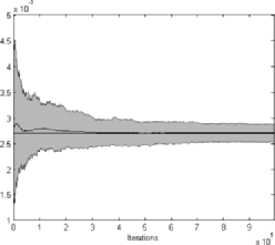
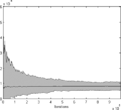
In order to further describe the Jeffreys prior, we use the algorithm to approximate the probability of the largest ball contained in $\mathcal{B}$ with respect to the Euclidean distance on $\mathcal{B}$. This distance may be computed using the Frobenius inner product described in the previous section. The largest ball has radius $1/(m-1)$, where $m>1$ is the size of the doubly stochastic matrix. Although this probability can be obtained exactly for the uniform distribution, we nevertheless approximate it using our algorithm, meanwhile providing some validation of the MCMC algorithm. Figure 1 shows the results we get for $m=4$.

(a)	(b)

Figure 1: Convergence of 1000 parallel MCMC runs for the probability of the largest ball contained in the polytope $\mathcal{B}$ with $m=4$. Shaded region represents the range of the entire set of approximations at each iteration. Figure (a) is the convergence for the probability in the case of the uniform distribution. The flat line, in this case, corresponds to the true probability $p\approx 0.0027$. Figure (b) is the same for the Jeffreys prior.

Notice that this probability is much smaller for the Jeffreys prior, because it distributes more mass towards the extremities of the polytope than the uniform prior does. This may also be observed by plotting the density estimates of the radius of the doubly stochastic matrix, that is, the Euclidean distance of the doubly stochastic matrix from the center of the polytope $\mathcal{B}$. These are shown in Figure 2.

(a)	(b)
(c)	(d)

Figure 2: Plots of samples and density estimates of the radius (Euclidean distance of the doubly stochastic matrix from the center of the polytope $\mathcal{B}$), on the interval $[0,q_{95}]$, where $q_{95}$ is the 95th quantile of its distribution. Figures (a) and (b) are results when sampling from the uniform prior and figures (c) and (d) are those of the Jeffreys prior. Here $m=4$.

5 Simulation experiments

The goal of the experiment is to study the performance of our estimator on artificial data sets generated from various bivariate distributions. We provide evidence that the estimators derived from our model give good results in general, and most important, that the Jeffreys prior is a reasonable choice.

Six parametric families of copulas are considered: [

• 1.]Clayton family: $C_{\theta}(u,v)=\{\max(0,u^{-\theta}+v^{-\theta}-1)\}^{-1/\theta},\ \theta\geq-1,\theta\neq 0,$

• Gumbel family: $C_{\theta}(u,v)=\exp[-\{(-\log u)^{\theta}+(-\log v)^{\theta}\}^{1/\theta}],\ \theta\geq 1,$

• Frank family: $C_{\theta}(u,v)=-\frac{1}{\theta}\log\{1+\frac{(\mathrm{e}^{-\theta u}-1)(\mathrm{e}^{-\theta v}-1)}{\mathrm{e}^{-\theta}-1}\},\ \theta\neq 0,$

• Gaussian family: $C_{\theta}(u,v)=\Phi_{\theta}(\Phi^{-1}(u),\Phi^{-1}(v)),\ |\theta|\leq 1,$ where $\Phi_{\theta}$ is the standard bivariate Gaussian cumulative distribution function with correlation coefficient $\theta$, and $\Phi^{-1}$ is the inverse of the univariate standard normal cumulative distribution function.

• Gaussian cross family: $C_{\theta}^{\times}(u,v)=1/2(C_{\theta}(u,v)-C_{\theta}(u,1-v)+u),\ |\theta|\leq 1$, where $C_{\theta}$ belongs to the Gaussian family.

• Gaussian diamond family:

  $$C_{\theta}^{\diamond}(u,v)=\cases{C_{\theta}^{\times}(u+1/2,v)-C_{\theta}^{\times}(1/2,v),&\quad if $u\leq 1/2$,\cr C_{\theta}^{\times}(u-1/2,v)+v-C_{\theta}^{\times}(1/2,v),&\quad if $u>1/2$,}$$

  where $|\theta|\leq 1$ and $C_{\theta}^{\times}$ belongs to the Gaussian cross family.

(a)	(b)

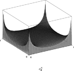
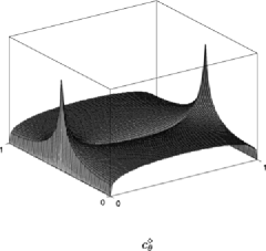
Figure 3: Densities of the Gaussian cross copula and the Gaussian diamond copula with $\theta=0.5$.

For the Clayton, Frank and Gaussian families, values of the parameter away from 0 indicate departure from independence, while a parameter away from 1 indicates departure from independence for the Gumbel family. These four families are among the popular ones in the literature, but the last two families are not, and so we now describe them in more detail. The Gaussian cross family is obtained by the following: Let $(U,V)$ be a random vector with uniform margins and with the Gaussian copula $C_{\theta}$ as its joint distribution. Let $W$ be an independent uniformly distributed random variable, and consider the random vector

$$(U_{\theta}^{\times},V_{\theta}^{\times})=(U,V)\mathbf{1}(W\leq 1/2)+(U,1-V)\mathbf{1}(W>1/2).$$

The distribution of $(U_{\theta}^{\times},V_{\theta}^{\times})$ is given by the Gaussian cross copula. Here, the superscript $\times$ is to highlight the “cross-like” dependence structure; see Figure 3(a) for a plot of its density when $\theta=0.5$. The Gaussian diamond family corresponds to the distributions of the random vectors

$$(U_{\theta}^{\diamond},V_{\theta}^{\diamond})=\bigl{(}U_{\theta}^{\times}+1/2(\mbox{mod }1),V_{\theta}^{\times}\bigr{)}\qquad\mbox{for each }|\theta|\leq 1.$$

See Figure 3(b) for an illustration of its density when $\theta=0.5$.

An extensive simulation experiment is carried out in two parts. In the first part, we consider the case of known marginal distributions and use bivariate data sampled from the copula families above. For each family, we consider 11 models corresponding to equally spaced parameter values in some interval. For the first four families, the interval is determined so that the Kendall’s $\tau$ values associated to the particular models range between 0 and $2/3$; see the simulation in Silva and Lopes [27]. Kendall’s $\tau$ associated with a copula $C$ is the dependence measure defined by

$$\tau=4\int_{0}^{1}\int_{0}^{1}C(u,v)\,\mathrm{d}C(u,v)-1.$$

The values of Kendall’s $\tau$ for the first four families are respectively given by $\tau=\theta/(\theta+2)$, $\tau=1-1/\theta$, $\tau=1-(4/\theta)[1-D_{1}(\theta)]$, where $D_{1}$ is the Debye function and $\tau=(2/\pi)\arcsin(\theta)$. For families 5 and 6, we consider the models corresponding to 11 values of $\theta$ ranging between 0 and 1. In the second part of the experiment, we simulate an unknown margins situation. We focus on families 4, 5 and 6 and consider 11 equally spaced values of $\theta$ ranging between 0 and 1 for the copula models. Here, a Student $t$ with seven degrees of freedom and a chi-square with four degrees of freedom are considered as the first and second margins, respectively.

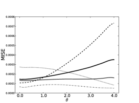
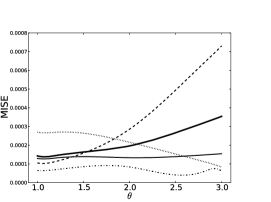
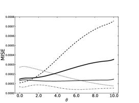
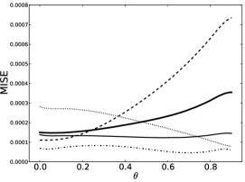
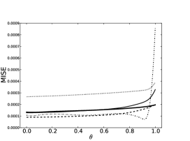
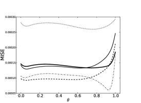
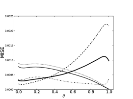
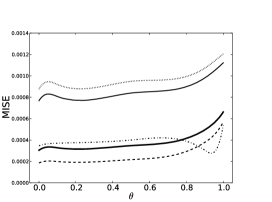
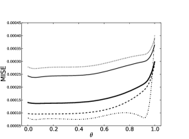
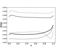
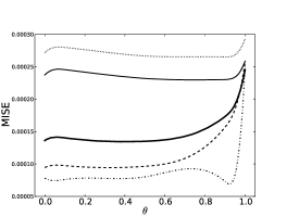
In the experiment, 1000 samples of both sizes $n=30$ and $n=100$ are generated from each model. For every data set, the copula function is estimated using five estimators. The first two are the Bayes estimators associated to the Jeffreys and the uniform priors, respectively. For the uniform prior, we mean the uniform distribution on $\mathcal{B}^{\prime}$ defined in Section 3, we use the bijection $\mathcal{B}=m^{-1}\mathbf{1}\mathbf{1}^{\top}+G\mathcal{B}^{\prime}G^{\top}$ given by expression (9). The third estimator is the maximum likelihood estimator (MLE) from our model $C_{\hat{P}}^{*}$, where $\hat{P}$ maximizes the likelihood derived from expression (7). This estimator is evaluated numerically. For the above three estimators, we take $m=6$ as the order of the doubly stochastic matrix in our model. Finally, we consider the two frequentist estimators, that is, Deheuvels’ estimator given in Theorem 3 and the Gaussian kernel estimator described in the Introduction. Values of the bandwidth for the latter estimator are based on the commonly used rule of thumb: $h=s_{i}n^{-1/5}$, where $s_{i}$, $i=1,2$, is the sample standard deviation of the $i$th margin; see Fermanian and Scaillet [8] and Sheather [26]. Figures 4, 5 and 6 report the values of the mean integrated squared errors,

$$\operatorname{MISE}(\widehat{C})=\mathrm{E}\biggl{[}\int_{0}^{1}\int_{0}^{1}\bigl{(}\widehat{C}(u,v)-C(u,v)\bigr{)}^{2}\,\mathrm{d}u\,\mathrm{d}v\biggr{]},$$

for the five estimators as a function of the parameter $\theta$.

(a) Family 1	(b) Family 2
(c) Family 3	(d) Family 4
(e) Family 5	(f) Family 6

Figure 4: Plots of MISE against $\theta$ in the known margins case. The MISE is approximated using 1000 samples of size $n=30$. Thick solid line is the MISE of the Bayes estimator using the Jeffreys prior, dashed line is that of the Bayes estimator using the uniform prior, dashed–dotted line is the MISE of the MLE, while dotted and thin solid line is the MISE of Deheuvels’ and the Gaussian kernel estimators, respectively.

(a) Family 1	(b) Family 2
(c) Family 3	(d) Family 4
(e) Family 5	(f) Family 6

Figure 5: Plots of MISE against $\theta$ in the known margins case. The MISE is approximated using 1000 samples of size $n=100$. Thick solid line is the MISE of the Bayes estimator using the Jeffreys prior, dashed line is that of the Bayes estimator using the uniform prior, dashed–dotted line is the MISE of the MLE, while dotted and thin solid line is the MISE of Deheuvels’ and the Gaussian kernel estimator, respectively.

(a) Model 4, $n=30$	(b) Model 4, $n=100$
(c) Model 5, $n=30$	(d) Model 5, $n=100$
(e) Model 6, $n=30$	(f) Model 6, $n=100$

Figure 6: Plots of MISE against $\theta$ in the unknown margins case. The MISE is approximated using 1000 samples each of sizes $n=30$ and $n=100$. Thick solid line is the MISE of the Bayes estimator using the Jeffreys prior, dashed line is that of the Bayes estimator using the uniform prior, dashed–dotted line is the MISE of the MLE, while dotted and thin solid line is the MISE of Deheuvels’ and the Gaussian kernel estimators, respectively.

As the results indicate, the Bayesian approach outperforms Deheuvels’ estimator and the kernel estimator near independence for the Clayton, Gumbel, Frank and Gaussian families. Unfortunately, this is not necessarily the case when the value of the parameter increases, that is, when the true copula approaches the Fréchet–Hoeffding upper bound, also called the comonotone copula, corresponding to (almost sure) perfect positive linear dependence. For families 5 and 6, the Bayes estimators outperform both frequentist estimators when the sample size is small ($n=30$). One remarkable feature that appears when comparing the results obtained in the known margins case with the results obtained in the unknown margins case is the decrease in performance of the kernel estimator. Recall that the latter estimator is the only one for which the invariance property mentioned in the Introduction does not hold. The other estimators seem to behave similarly when comparing their resulting MISE in the known margins case with their MISE in the unknown margins case. Notice the resemblance in shape of the MISE for Deheuvels’ estimator and the kernel estimator in the unknown margins cases. Finally, the performance of the MLE is worth mentioning, since in many cases it has the smallest MISE, especially for large values of $\theta$. This is because the MLE will go on the boundary of the parameter space easily, while the Bayes estimator will always stay away from the boundary with the types of priors that we have selected. However, if such an extreme case is to happen in a real life problem, it is probable that the practitioner has some insight on the phenomenon beforehand, and may choose to work with a more appropriate (subjective) prior.

6 Discussion

Two points need to be further discussed. First, our methodology is purely Bayesian only when the marginal distributions are known. When these are unknown, our methodology is empirical Bayes. In fact, in this case we propose a two-step procedure by first estimating the marginsvia the empirical marginal distributions and then plugging them in as the true distributions thereafter. We have chosen to do this because it is common practice to do so (see Genest et al. [11]), it is simple to implement, it is robust against outliers and our estimator is consequently invariant under increasing transformations of the margins. One way to propose a purely Bayesian estimator by using our model for the copula is to use finite mixtures for the margins. This way, if the densities used in the latter mixtures have disjoint supports, then the Jeffreys prior for the mixing weights has a simple form and is proper; see Bernardo and Girón [2]. Now by selecting independent Jeffreys priors for the margins and for the copula, the resulting prior is proper as well.

Finally, our models given by the approximation spaces $\mathcal{C}_{m}$, $m>1$, are called sieves by some authors; see Grenander [13]. In the present paper, we have chosen to work with a fixed sieve, so this makes our model finite dimensional. In this case, the methodology falls in the semi-parametric approach described in the Introduction. Here, the rather subjective choice of the sieve to work with can be viewed as a weakness of the proposed methodology. On the other hand, by using the entire set of sieves, we can construct a nonparametric model for the copula that can, in some sense, respect the infinite-dimensional nature of the copula functions. In fact, if we take $\mathcal{C}=\bigcup_{m>1}\mathcal{C}_{m}$, then $\mathcal{C}$ is dense in the space of copulas. Our Bayesian methodology can be easily adapted here. This can be achieved by selecting an infinite support prior for the model index $m$ and using our methodology inside each model. The Bayesian estimator becomes an infinite mixture of the estimators proposed in this paper (one for each model $m$), where the mixing weights are given by the posterior probabilities of the models.

Appendix

Proof of Lemma 4 Here we show how to compute $I(W)=\det(\mathrm{E}[\frac{-\partial^{2}\log c_{P}^{*}(u,v)}{\partial W^{2}}])$ efficiently. First, notice that $A=\mathrm{E}[\frac{-\partial^{2}\log c_{P}^{*}(u,v)}{\partial W^{2}}]$ can be written as $A=D_{0}^{-1}+CD_{1}^{-1}C^{\top},$ where

$$D_{0} = \operatorname{diag}\bigl{(}w_{11},\ldots,w_{1(m-1)},\ldots,w_{(m-1)1},\ldots,w_{(m-1)(m-1)}\bigr{)},$$

$$D_{1} = \operatorname{diag}\bigl{(}w_{mm},w_{1m},\ldots,w_{(m-1)m},w_{m1},\ldots,w_{m(m-1)}\bigr{)}$$

and

$$C_{(m-1)^{2}\times(2m-1)}=\pmatrix{\mathbf{1}_{m-1}&\mathbf{1}_{m-1}&0\mathbf{1}_{m-1}&\cdots&I_{m-1}\cr\mathbf{1}_{m-1}&0\mathbf{1}_{m-1}&\mathbf{1}_{m-1}&\cdots&I_{m-1}\cr\mathbf{1}_{m-1}&0\mathbf{1}_{m-1}&0\mathbf{1}_{m-1}&\cdots&I_{m-1}\cr\vdots&\vdots&\vdots&\vdots&\vdots\cr\mathbf{1}_{m-1}&0\mathbf{1}_{m-1}&0\mathbf{1}_{m-1}&\cdots&I_{m-1}\cr}.$$

Thus, $\det A=\det(D_{1}+C^{\top}D_{0}C)/(\det D_{0}\det D_{1})$. If we let $B=(w_{ij})_{i,j=1,\ldots,m-1}$, then since $\sum_{i=1}^{m}w_{ij}=1/m$, for all $j=1,\ldots,m$, and $\sum_{j=1}^{m}w_{ij}=1/m$ for all $i=1,\ldots,m$,

$$D_{1}+C^{\top}D_{0}C=\pmatrix{1-2(1/m-w_{mm})&\mathbf{1}^{\top}B^{\top}&\mathbf{1}^{\top}B\cr B\mathbf{1}&(1/m)I&B\cr B^{\top}\mathbf{1}&B^{\top}&(1/m)I\cr}.$$

By elementary row and column operations, we get

$$\det(D_{1}+C^{\top}D_{0}C)=\det\pmatrix{1&(1/m)\mathbf{1}^{\top}&(1/m)\mathbf{1}^{\top}\cr(1/m)\mathbf{1}&(1/m)I&B\cr(1/m)\mathbf{1}&B^{\top}&(1/m)I\cr},$$

so that

$$\det(D_{1}+C^{\top}D_{0}C)$$

$$\quad=\det\left(\pmatrix{(1/m)I&B\cr B^{\top}&(1/m)I}-(1/m^{2})\mathbf{1}_{2(m-1)}\mathbf{1}_{2(m-1)}^{\top}\right)$$

$$\quad=\det\pmatrix{(1/m)\bigl{(}I-(1/m)\mathbf{1}\mathbf{1}^{\top}\bigr{)}&B-(1/m^{2})\mathbf{1}\mathbf{1}^{\top}\cr B^{\top}-(1/m^{2})\mathbf{1}\mathbf{1}^{\top}&(1/m)\bigl{(}I-(1/m)\mathbf{1}\mathbf{1}^{\top}\bigr{)}}$$

$$\quad=\det\bigl{(}(1/m)\bigl{(}I-(1/m)\mathbf{1}\mathbf{1}^{\top}\bigr{)}\bigr{)}\det\bigl{(}\bigl{[}(1/m)\bigl{(}I-(1/m)\mathbf{1}\mathbf{1}^{\top}\bigr{)}\bigr{]}$$

$$\qquad\phantom{\det\bigl{(}}{}-[B^{\top}-(1/m^{2})\mathbf{1}\mathbf{1}^{\top}]\bigl{[}(1/m)\bigl{(}I-(1/m)\mathbf{1}\mathbf{1}^{\top}\bigr{)}\bigr{]}^{-1}[B-(1/m^{2})\mathbf{1}\mathbf{1}^{\top}]\bigr{)}.$$

Finally, $\det((1/m)(I-(1/m)\mathbf{1}\mathbf{1}^{\top}))=(1/m)^{m}\mbox{ and }[(1/m)(I-(1/m)\mathbf{1}\mathbf{1}^{\top})]^{-1}=m(I+\mathbf{1}\mathbf{1}^{\top})$, thus

$$\det(D_{1}+C^{\top}D_{0}C)=(1/m)^{m}\det\bigl{(}(1/m)I-mV^{\top}V\bigr{)},$$

where $V=(w_{ij})_{i=1,\ldots,m;j=1,\ldots,m-1}$.

Proof of Theorem 1 We prove that the Jeffreys prior is proper. Consider the following partition of $V$, $V=(V_{1}V_{2}\cdots V_{m-1})$, where each $V_{j}$ is a vector, $j=1,\ldots,m-1$. The matrix $(1/m)I-mV^{\top}V$ is symmetric, non-negative and semi-definite, so that by Hadamard’s inequality, we have

$$\det\bigl{(}(1/m)I-mV^{\top}V\bigr{)} \leq \prod_{j=1}^{m-1}(1/m-m\|V_{j}\|^{2})$$

$$= \prod_{j=1}^{m-1}\biggl{(}2m\sum_{1\leq i<k\leq m}w_{ij}w_{kj}\biggr{)}$$

$$= (2m)^{m-1}\sum_{1\leq i_{m-1}<k_{m-1}\leq m}\cdots\sum_{1\leq i_{1}<k_{1}\leq m}\prod_{j=1}^{m-1}w_{i_{j}j}w_{k_{j}j}.$$

For any $W\in\mathcal{W}$, we have

$$\sqrt{I(W)} = \sqrt{\det\bigl{(}(1/m)I-mV^{\top}V\bigr{)}}\Big{/}\sqrt{m^{m}\prod_{i,j=1}^{m}w_{ij}}$$

$$\leq \sqrt{2^{m-1}/m}\Biggl{\{}\sum_{1\leq i_{m-1}<k_{m-1}\leq m}\cdots\sum_{1\leq i_{1}<k_{1}\leq m}\prod_{j=1}^{m-1}w_{i_{j}j}w_{k_{j}j}\Biggr{\}}^{1/2}\bigg{/}\sqrt{\prod_{i,j=1}^{m}w_{ij}}$$

$$\leq \sqrt{2^{m-1}/m}\sum_{1\leq i_{m-1}<k_{m-1}\leq m}\cdots\sum_{1\leq i_{1}<k_{1}\leq m}\Biggl{\{}\prod_{j=1}^{m-1}w_{i_{j}j}w_{k_{j}j}\Biggr{\}}^{1/2}\bigg{/}\sqrt{\prod_{i,j=1}^{m}w_{ij}}$$

$$= \sqrt{2^{m-1}/m}\sum_{\alpha\in\mathcal{A}}\prod_{i,j=1}^{m}w_{ij}^{\alpha_{ij}-1},$$

where $\mathcal{A}=\{\alpha_{ij}\in\{1/2,1\}\colon\ i,j=1,\ldots,m,\alpha_{+j}=m/2+1,j=1,\ldots,m-1\mbox{ and }\alpha_{+m}=m/2\},$ with $\alpha_{+j}=\sum_{i=1}^{m}\alpha_{ij}$, for all $j=1,\ldots,m$. We need to show that the integral of $\prod_{i,j=1}^{m}w_{ij}^{\alpha_{ij}-1}$ is finite for all $\alpha\in\mathcal{A}$. The integration is made with respect to $w_{ij},i\vee j<m$, the free variables. For any permutation matrices $P_{1}$ and $P_{2}$, the transformation $W\mapsto P_{1}WP_{2}$ is a one-to-one transformation from $\mathcal{W}$ onto $\mathcal{W}$, and the Jacobian, in absolute value, is equal to one. Therefore, it is sufficient to verify that the integral of $\prod_{i,j=1}^{m}w_{ij}^{\alpha_{ij}-1}$ is finite for all $\alpha\in\mathcal{A}_{0}$, where $\mathcal{A}_{0}=\{\alpha\in\mathcal{A}\colon\ \alpha_{m-1m}=\alpha_{mm}=1\}.$ The idea is to decompose the multiple integral into $m-2$ iterated integrals over the sections given by

$$\mathcal{W}_{k}=\{w_{ij}\geq 0\colon\ i\wedge j=k,i\vee j\leq m,w_{k+}=w_{+k}=1/m\},\qquad k=1,\ldots,m-2,$$

and

$$\mathcal{W}_{m-1}=\{w_{ij}\geq 0\colon\ i,j=m-1,m,w_{m-1+}=w_{+m-1}=w_{m+}=w_{+m}=1/m\}.$$

Here, the set $\mathcal{W}_{1}$ is fixed, the sets $\mathcal{W}_{k}$ are parameterized by $\{w_{ij}\geq 0\colon\ i\wedge j<k,i\vee j=k\}$, $k=2,\ldots,m-2$, and $\mathcal{W}_{m-1}$ is parameterized by $\{w_{ij}\geq 0\colon\ i\wedge j<m-1,i\vee j=m-1,m\}$. By Fubini’s theorem, for any non-negative function $f$, we can write

$$\int_{\mathcal{W}}f(W)\prod_{i,j=1}^{m-1}\mathrm{d}w_{ij}=\int_{\mathcal{W_{1}}}\biggl{\{}\cdots\int_{\mathcal{W_{m-1}}}\{f(W)\,\mathrm{d}w_{m-1m-1}\}\cdots\biggr{\}}\prod_{i\wedge j=1,i\vee j<m}\mathrm{d}w_{ij}.$$

The next step consists in finding finite functions $c_{k}$, $k=1,\ldots,m-1$, on $\mathcal{A}_{0}$, such that

$$\int_{\mathcal{W_{k}}}\prod_{i\wedge j=k,i\vee j\leq m}w_{ij}^{\alpha_{ij}-1}\prod_{i\wedge j=k,i\vee j<m}\mathrm{d}w_{ij}\leq c_{k}(\alpha),$$

for all $\alpha\in\mathcal{A}_{0}$, uniformly on $\{w_{ij}\geq 0\colon\ i\wedge j<k,i\vee j=k\}$, for $k=1,\ldots,m-2$, and uniformly on $\{w_{ij}\,{\geq}\,0\colon\ i\,{\wedge}\,j\,{<}\,m\,{-}\,1,i\,{\vee}\,j\,{=}\,m\,{-}\,1,m\}$, for $k\,{=}\,m\,{-}\,1$. This will give us that

$$\int_{\mathcal{W}}\prod_{i,j\leq m}w_{ij}^{\alpha_{ij}-1}\prod_{i,j<m}\mathrm{d}w_{ij}\leq\prod_{k=1}^{m-1}c_{k}(\alpha),$$

for all $\alpha\in\mathcal{A}_{0}$.

Let $a=0\vee\{\sum_{\ell<m-1}(w_{\ell m}-w_{m-1\ell})\}\vee\{\sum_{\ell<m-1}(w_{m\ell}-w_{\ell m-1})\}$ and $b=1/m-\{(\sum_{\ell<m-1}w_{\ell m-1})\vee(\sum_{\ell<m-1}w_{m-1\ell})\}$. If $a>b$, the set $\mathcal{W}_{m-1}$ is empty. Suppose that $\mathcal{W}_{m-1}$ is not empty and $\alpha\in\mathcal{A}_{0}$. Let $b_{0}=1/m-\sum_{\ell<m-1}w_{\ell m-1}$. We have

$$\int_{\mathcal{W_{m-1}}}\prod_{i,j=m-1,m}w_{ij}^{\alpha_{ij}-1}\,\mathrm{d}w_{m-1m-1} = \int_{a}^{b}u^{\alpha_{m-1m-1}-1}(b_{0}-u)^{\alpha_{mm-1}-1}\,\mathrm{d}u$$

$$\leq \int_{0}^{b_{0}}u^{\alpha_{m-1m-1}-1}(b_{0}-u)^{\alpha_{mm-1}-1}\,\mathrm{d}u$$

$$= b_{0}^{\alpha_{m-1m-1}+\alpha_{mm-1}-1}B(\alpha_{m-1m-1},\alpha_{mm-1})$$

$$\leq B(\alpha_{m-1m-1},\alpha_{mm-1})$$

$$= c_{m-1}(\alpha).$$

For $k=1,\ldots,m-2$ and $\alpha\in\mathcal{A}_{0}$ we can take

$$c_{k}(\alpha)=\Biggl{(}B\Biggl{(}\alpha_{kk},\sum_{i=k+1}^{m}\alpha_{ik}\Biggr{)}+B\Biggl{(}\alpha_{kk},\sum_{j=k+1}^{m}\alpha_{kj}\Biggr{)}\Biggr{)}\frac{\prod_{i>k}\Gamma(\alpha_{ik})\prod_{j>k}\Gamma(\alpha_{kj})}{\Gamma(\sum_{i>k}\alpha_{ik})\Gamma(\sum_{j>k}\alpha_{kj})}.$$

The justification is given by Lemma 5.

Lemma 5

If $0<a,b\leq 1,m\geq 3,\alpha>0$,

$$\beta_{j} > 0,\qquad j=1,\ldots,m-1,\qquad\mbox{with }\beta=\sum_{j=1}^{m-1}\beta_{j}\geq 1,$$

$$\gamma_{i} > 0,\qquad i=1,\ldots,m-1,\qquad\mbox{with }\gamma=\sum_{i=1}^{m-1}\gamma_{i}\geq 1$$

and

$$C=\Biggl{\{}w_{ij}\geq 0\colon\ i\wedge j=1,i\vee j\leq m,\sum_{j=1}^{m}w_{1j}=a,\sum_{i=1}^{m}w_{i1}=b\Biggr{\}},$$

then

$$\int_{C}w_{11}^{\alpha-1}\prod_{j=2}^{m}w_{1j}^{\beta_{j-1}-1}\prod_{i=2}^{m}w_{i1}^{\gamma_{i-1}-1}\,\mathrm{d}w_{11}\prod_{j=2}^{m-1}\mathrm{d}w_{1j}\prod_{i=2}^{m-1}\mathrm{d}w_{i1}$$

$$\quad\leq\bigl{(}B(\alpha,\beta)+B(\alpha,\gamma)\bigr{)}\frac{\prod_{j=1}^{m-1}\Gamma(\beta_{j})\prod_{i=1}^{m-1}\Gamma(\gamma_{i})}{\Gamma(\beta)\Gamma(\gamma)}.$$

[Proof.] Let

$$K(a,b,\alpha,\beta,\gamma)=\int_{0}^{a\wedge b}w^{\alpha-1}(a-w)^{\beta-1}(b-w)^{\gamma-1}\,\mathrm{d}w.$$

If $a<b$, then

$$K(a,b,\alpha,\beta,\gamma) = \int_{0}^{a}w^{\alpha-1}(a-w)^{\beta-1}(b-w)^{\gamma-1}\,\mathrm{d}w$$

$$\leq b^{\gamma-1}\int_{0}^{a}w^{\alpha-1}(a-w)^{\beta-1}\,\mathrm{d}w$$

$$= a^{\alpha+\beta-1}b^{\gamma-1}B(\alpha,\beta)\leq B(\alpha,\beta).$$

In the same way, if $b<a$, then $K(a,b,\alpha,\beta,\gamma)\leq B(\alpha,\gamma)$, so that

$$K(a,b,\alpha,\beta,\gamma)\leq B(\alpha,\beta)+B(\alpha,\gamma).$$ (11)

Now, let $W_{11}$ be a random variable on $(0,a\wedge b)$ with density

$$\frac{1}{K(a,b,\alpha,\beta,\gamma)}w_{11}^{\alpha-1}(a-w_{11})^{\beta-1}(b-w_{11})^{\gamma-1},$$

let $(U_{12},\ldots,U_{1m})$ be a random vector distributed according to a $\operatorname{Dirichlet}(\beta_{1},\ldots,\beta_{m-1})$, let $(U_{21},\ldots,U_{m1})$ be distributed according to a $\operatorname{Dirichlet}(\gamma_{1},\ldots,\gamma_{m-1})$ and further assume independence between $W_{11}$, $(U_{12},\ldots,U_{1m})$ and $(U_{21},\ldots,U_{m1})$. Let $W_{1j}=(a-W_{11})U_{1j},$ $j=2,\ldots,m,$ and $W_{i1}=(b-W_{11})U_{i1},$ $i=2,\ldots,m.$ From this construction, given $W_{11}=w_{11}$, we have that $(W_{12},\ldots,W_{1m})$ and $(W_{21},\ldots,W_{m1})$ are conditionally independent with conditional densities given, respectively, by

$$\frac{1}{(a-w_{11})^{\beta-1}}\frac{\Gamma(\beta)}{\prod_{i=1}^{m-1}\Gamma(\beta_{i})}w_{12}^{\beta_{1}-1}\cdots w_{1m}^{\beta_{m-1}-1},$$

with $w_{1j}\geq 0$, $j=2,\ldots,m$, $\sum_{2\leq j\leq m}w_{1j}=a-w_{11}$ and

$$\frac{1}{(b-w_{11})^{\gamma-1}}\frac{\Gamma(\gamma)}{\prod_{i=1}^{m-1}\Gamma(\gamma_{i})}w_{21}^{\gamma_{1}-1}\cdots w_{m1}^{\gamma_{m-1}-1},$$

with $w_{i1}\geq 0$, $i=2,\ldots,m$, $\sum_{2\leq i\leq m}w_{i1}=b-w_{11}$. This construction, together with inequality (11), implies the result, namely

$$\int_{C}w_{11}^{\alpha-1}\prod_{j=2}^{m}w_{1j}^{\beta_{j-1}-1}\prod_{i=2}^{m}w_{i1}^{\gamma_{i-1}-1}\,\mathrm{d}w_{11}\prod_{j=2}^{m-1}\mathrm{d}w_{1j}\prod_{i=2}^{m-1}\mathrm{d}w_{i1}$$

$$\quad\leq\bigl{(}B(\alpha,\beta)+B(\alpha,\gamma)\bigr{)}\frac{\prod_{j=1}^{m-1}\Gamma(\beta_{j})\prod_{i=1}^{m-1}\Gamma(\gamma_{i})}{\Gamma(\beta)\Gamma(\gamma)}.$$

Lemma 6

Consider $X$, a $\operatorname{Binomial}(n,p)$ random variable. We have

$$\sup_{0\leq p\leq 1}\mathrm{E}_{p}[|X-np|]=\cases{1/B\bigl{(}1/2,(n+1)/2\bigr{)},&\quad if $n$ is odd,\cr\bigl{(}1-(n+1)^{-2}\bigr{)}^{n/2}\bigl{(}1+(n+1)^{-2}\bigr{)}1/B(1/2,n/2),&\quad if $n$ is even.}$$

[Proof.] Let $\mu_{n}(p)=\mathrm{E}_{p}[|X-np|].$ We have

$$\mu_{n}(p)=\frac{2n!}{(\lfloor np\rfloor)!(n-1-\lfloor np\rfloor)!}p^{\lfloor np\rfloor+1}(1-p)^{n-\lfloor np\rfloor}\qquad\mbox{for all }n\geq 1,p\in[0,1],$$

where $\lfloor x\rfloor=\max\{n\colon\ n\leq x,n\mbox{ is an integer}\}$ for all $x$. Therefore,

$$\sup_{0\leq p\leq 1}\mu_{n}(p) = \max_{0\leq k\leq n-1}\sup_{\{p\colon\ \lfloor np\rfloor=k\}}\mu_{n}(p)$$

$$= \max_{0\leq k\leq n-1}\mu_{n}\biggl{(}\frac{k+1}{n+1}\biggr{)},$$

and, in particular, $\sup_{0\leq p\leq 1}\mu_{1}(p)\,{=}\,\mu_{1}(1/2)\,{=}\,1/2\,{=}\,1/B(1/2,1)$. Now assume that $n\,{>}\,1$. Let

$$\nu_{n}(k)=\mu_{n}\biggl{(}\frac{k+2}{n+1}\biggr{)}\Big{/}\mu_{n}\biggl{(}\frac{k+1}{n+1}\biggr{)},$$

for $k=0,\ldots,n-2$. We have

$$\nu_{n}(k)=\frac{(1+(k+1)^{-1})^{k+2}}{(1+(n-k-1)^{-1})^{n-k}}\quad\mbox{and}\quad\nu_{n}(k)=\frac{1}{\nu_{n}(n-2-k)}\qquad\mbox{for }k=0,\ldots,n-2.$$

However,

$$\frac{d}{dt}\log\biggl{(}1+\frac{1}{t}\biggr{)}^{t+1}=\log\biggl{(}1+\frac{1}{t}\biggr{)}-\frac{1}{t}<0\qquad\mbox{for all }t>1.$$

This implies that $\nu_{n}$ decreases on $\{0,\ldots,n-2\}.$ Therefore,

$$\mu_{n}\biggl{(}\frac{1}{n+1}\biggr{)} < \cdots<\mu_{n}\biggl{(}\frac{(n+1)/2}{n+1}\biggr{)}>\cdots>\mu_{n}\biggl{(}\frac{n}{n+1}\biggr{)}\qquad\mbox{if }n\mbox{ is odd,}$$

$$\mu_{n}\biggl{(}\frac{1}{n+1}\biggr{)} < \cdots<\mu_{n}\biggl{(}\frac{n/2}{n+1}\biggr{)}=\mu_{n}\biggl{(}\frac{n/2+1}{n+1}\biggr{)}>\cdots>\mu_{n}\biggl{(}\frac{n}{n+1}\biggr{)}\qquad\mbox{if }n\mbox{ is even.}$$

The final expression is obtained using the following identity:

$$n!=2^{n}\Gamma\biggl{(}\frac{n}{2}+1\biggr{)}\Gamma\biggl{(}\frac{n+1}{2}\biggr{)}\Big{/}\Gamma\biggl{(}\frac{1}{2}\biggr{)}\qquad\mbox{for all }n\geq 0.$$