The International-Trade Network:
Gravity Equations and Topological Properties
Abstract
This paper begins to explore the determinants of the topological properties of the international - trade network (ITN). We fit bilateral-trade flows using a standard gravity equation to build a “residual” ITN where trade-link weights are depurated from geographical distance, size, border effects, trade agreements, and so on. We then compare the topological properties of the original and residual ITNs. We find that the residual ITN displays, unlike the original one, marked signatures of a complex system, and is characterized by a very different topological architecture. Whereas the original ITN is geographically clustered and organized around a few large-sized hubs, the residual ITN displays many small-sized but trade-oriented countries that, independently of their geographical position, either play the role of local hubs or attract large and rich countries in relatively complex trade-interaction patterns.
pacs:
89.75.-k, 89.65.Gh, 87.23.Ge, 05.70.Ln, 05.40.-aI Introduction
The last years have witnessed the emergence of a large body of contributions addressing international-trade issues from a complex-network perspective (Li et al., 2003; Serrano and Boguñá, 2003; Garlaschelli and Loffredo, 2004, 2005; Reichardt and White, 2007; Serrano et al., 2007; Bhattacharya et al., 2008, 2007; Garlaschelli et al., 2007; Tzekina et al., 2008; Fagiolo et al., 2008; Reyes et al., 2008; Fagiolo et al., 2009a). The International Trade Network (ITN), aka World-Trade Web (WTW) or World-Trade Network (WTN), is defined as the graph of import/export relationships between world countries in a given year.
Understanding the topological properties of the ITN, and their evolution over time, acquires a fundamental importance in explaining issues such as economic globalization and internationalization, the spreading of international crises, and the transmission of economic shocks, for two related reasons (Helliwell and Padmore, 1985; Artis et al., 2003; Forbes, 2002). On the one hand, direct (bilateral) trade linkages are known to be one of the most important channels of interaction between world countries (Krugman, 1995). On the other hand, they can only explain a small fraction of the impact that an economic shock originating in a given country can have on another one, which is not among its direct-trade partners (Abeysinghe and Forbes, 2005). Therefore, a complex-network analysis (Albert and Barabási, 2002; Dorogovtsev and Mendes, 2003) of the ITN, by characterizing in detail the topological structure of the network, can go far beyond the scope of standard international-trade indicators (such as “openness to trade” 111Traditionally measured by the ratio of exports plus imports to country’s gross domestic product (GDP).), which instead only account for bilateral-trade direct linkages (Reyes et al., 2008). Trade paths connecting any pair of non-direct trade partners may then shed light on the likelihood that economic shocks might be transmitted between the two countries (Kali and Reyes, 2007), and possibly help explaining macroeconomic dynamics (Kali et al., 2007).
The first stream of studies that have explored the properties of the ITN has employed a binary-network analysis, where a (possibly directed) link between any two countries is either present or not according to whether the value of the associated trade flow is larger than a given threshold (Serrano and Boguñá, 2003; Garlaschelli and Loffredo, 2004, 2005). More recently, however, a growing number of contributions (Li et al., 2003; Bhattacharya et al., 2008, 2007; Garlaschelli et al., 2007; Fagiolo et al., 2008; Fagiolo et al., 2009a) have adopted a weighted-network approach (Barrat et al., 2004; Barthélemy et al., 2005) to the study of the ITN. There, a link between any two countries is weighted by the (deflated) value of trade (imports plus exports) that has occurred between these countries in a given time interval. A set of weighted-network topological measures (Barthélemy et al., 2005) is then computed to characterize the architecture of the weighted ITN.
The motivation for a weighted-network analysis is that a binary approach cannot fully extract the wealth of information about the trade intensity flowing through each link and therefore might dramatically underestimate the role of heterogeneity in trade linkages. Interestingly, Refs. (Fagiolo et al., 2008; Fagiolo et al., 2009a) show that the statistical properties of the ITN viewed as a weighted network crucially differ from those exhibited by its weighted counterpart, and that a weighted-network analysis is able to provide a more complete and truthful picture of the ITN than a binary one.
Notwithstanding much is known about the topological properties of the ITN —in both its binary and weighted versions— and how they have evolved in the recent past, a set of fundamental questions remains to be answered: What are the determinants of such properties? Are there relevant node or link characteristics (other than the ones related to trade flows) that can explain the peculiar topological patterns actually observed in the ITN? Such questions might be in principle addressed from a theoretical perspective, i.e. looking for models of network formation and evolution that have as their equilibria graphs with properties similar to those actually observed in the ITN (cf. for example Refs. (Albert and Barabási, 2002; Jackson et al., 2003)). In this paper we take an applied approach and attempt to explore the foregoing issues from a more empirical perspective.
To begin with, note that all network-related topological variables are univocally obtained from the link-weight distribution 222For example, node strength, clustering coefficient, centrality, etc. are simple manipulations that require as inputs the link-weight distribution only. See Appendix C for formal definitions.. Hence, if (as typically happens) one weights the link between country and country in a given year by the sum of the deflated values of imports of from and exports of to in that year, then all topological properties of the weighted ITN defined in that way will entirely depend on the matrix of international bilateral-trade flows observed in the year under study, which plays the role of sufficient statistics. This is straightforward for the weighted-version of the ITN, but is also true for its binary representations, as the probability that a given link is present still depends, given the chosen threshold, on the distribution of observed bilateral-trade flows. As a result, one might safely conclude that much of what we know about the topological properties of the ITN can be empirically accounted for by the set of statistically-significant independent variables that explain international bilateral-trade flows.
In the context of the ITN literature, this issue has been initially addressed by Refs. (Garlaschelli and Loffredo, 2004; Garlaschelli et al., 2007), who have shown that the probability that any two countries are connected, as well as the value of the trade flow between them, is well explained by (the product of) their current GDP, which plays the role of a “hidden” node variable or fitness. More generally, we know from the huge empirical literature on gravity equations (Leamer and Levinsohn, 1995; Overman et al., 2003) that international-trade flows can be almost entirely explained by a multiplicative model featuring as independent variables the GDPs of the two countries involved in the trade link, their geographical distance (as a proxy of all factors that might create trade resistance, e.g. transport costs), and a series of dummies accounting for other geographical, social, historical and political factors (e.g., existence of common borders, religion and languages, colonial ties, trade agreements, and so on). By fitting a gravity equation to the original international bilateral-trade data one may then account for explanatory variables of link weights.
Such an exercise might be interesting for two related reasons. First, from a gravity-equation approach, one may identify what are the main determinants of international-trade flows in the data used to build trade networks. Second, and more importantly, one might think to remove all the existing structure from the data to check whether the residual weighted ITN exhibits topological features comparable to those of the original ITN.
This paper explores these two lines of inquiry by performing the following simple exercise. In line with the recent literature (Li et al., 2003; Bhattacharya et al., 2008, 2007; Garlaschelli et al., 2007; Fagiolo et al., 2008; Fagiolo et al., 2009a), we start from a weighted-network representation of the ITN in a given year where a link between any two countries is weighted by the (deflated) value of their total trade (import plus exports). We then fit total-trade flows, i.e. the entries of the ITN weight matrix, with a standard gravity model. This allows us to identify the relative impact of size, geographical distance, and other geographical, social, historical and political factors, on the weighted-network representation of the ITN under study. Finally, we build a “residual” version of the ITN where each link is now weighted by the associated residual of the fitted gravity model. This allows us to remove much of the structure that is conceivably present in the original data.
We ask whether —and to what extent— the topological properties of such a residual ITN mimic those of the original version of the ITN (as studied, e.g., in Ref. (Fagiolo, 2007)). Notice that a similar approach has been already used in Ref. (Fagiolo et al., 2009b). They find that, by and large, the ITN architecture remains unaltered if ones removes the GDP dependence only from link weights (e.g., if one employs as link weights the ratio between bilateral-trade flows divided by the GDP of either the importer or the exporter country). The gravity-equation fit allows us to generalize this approach and obtain a weighted ITN that depends on underlying factors, either unobserved or not accounted for in the regression, related e.g. to country technological similarities, degree of specialization, etc..
Our results show that the residual ITN is characterized by power-law shaped distributions of link weights and node statistics (e.g., strength, clustering, random-walk betweenness centrality). Hence, the underlying architecture of the weighted ITN seem to display signatures of complexity. This must be contrasted with the original ITN, where log-normal distributions were ubiquitous. We also find that the correlation structure among node statistics, and between node statistics and country per-capita GDP, changes substantially when comparing the original and residual weighted networks. Whereas the original ITN is geographically clustered and organized around a few large-sized hubs, the residual ITN features many small-sized but trade-oriented countries that, independently of their geographical position, either play the role of local hubs or attract large and rich countries in relatively complex trade-interaction patterns.
The rest of the paper is organized as follows. Section II briefly presents the data sets employed in the paper. Section III contains the results of gravity-equation fits. A comparison of the topological properties of the original and the “residual” version of the ITN is carried out in Section IV. Finally, Section V concludes discussing the implications of our results for modeling and suggesting extensions of the present work.
II Data and Definitions
We employ international-trade data provided by Ref. Gleditsch (2002) to build a time-sequence of weighted directed ITNs. Our balanced panel refers to years (1981-2000) and countries (see Appendix A for the list of acronyms and countries in the panel). For each country and year, data report directed trade flows (e.g., exports) in current US dollars, which we properly deflate. Weight matrices are built following the flow of goods. This means that rows represent exporting countries, whereas columns stand for importing countries. Following Refs. (Li et al., 2003; Bhattacharya et al., 2008, 2007; Garlaschelli et al., 2007), we begin by initially defining the weight of a link from to in year as total exports from to . However, a simple statistical analysis of weighted matrices suggests that are sufficiently symmetric to justify an undirected analysis for all (Fagiolo et al., 2009a). We therefore symmetrize the network by defining the entries of the new weight matrix as the arithmetic average of import and export flows, i.e. 333Following Ref. (Baldwin and Taglioni, 2006), we have also replicated our exercises by using a geometric average of bilateral flows without noticing relevant differences in the results.. Finally, in order to have (and to remove all trend-related factors), for all and , we re-normalize all entries in by their maximum value . This means that the symmetrized weight is proportional to total trade (imports plus exports) flowing through the link in a given year.
Note that Ref. (Fagiolo et al., 2009a) has shown that all topological properties of the ITN have remained fairly stable in the period 1981-2000. Therefore, in what follows, we shall focus on year 2000 only for the sake of exposition (all results robustly hold in other years). Our relevant ITN data is then the weight matrix , which is symmetric by construction and features only zeroes in its main diagonal.
For each country in the panel, we also gather a long list of variables traditionally employed in gravity-equation exercises, see Appendix B for labels, sources and explanations. These variables can be grouped in three classes. First, there are variables related to trade resistance factors, as the geographical distance between countries and the degree of country remoteness (Bhavnani et al., 2002). Second, country-size effects are controlled by country GDP, population and geographical area. Third, a number of country variables or link-related dummies control for geographical (common border, landlocking, continent), economic (trade agreements, exchange rates, consumer price indices) and social/ political/ historical effects (common languages and religion, trade agreements, common currency). Together, these factors have been shown to successfully explain, in a way or in the other, international-trade flows in gravity-equation econometric exercises. Therefore, in the next section, we shall employ a standard gravity-equation setup to explain the entries of the weight matrix characterizing the ITN graph in year 2000.
III Fitting Gravity Equations to ITN Data
The gravity equation has become the workhorse setup to study the determinants of bilateral international-trade flows (Overman et al., 2003; Fratianni, 2009). Its basic symmetric original formulation, inspired by Newton’s gravity equation, states that total trade between any two countries in the world is directly proportional to the product of country masses (e.g., their GDP) and inversely proportional to their geographic distance 444This empirically-inspired law has been found to be consistent with a number of theoretical foundations, e.g. trade specialization models, monopolistic-competition frameworks with intra-industry trade, Hecksher-Ohlin models, etc.; see, e.g., Refs. (Anderson, 1979; Bergstrand, 1985; Deardorff, 1998; Anderson and van Wincoop, 2003)..
A strong gravity-like dependence of bilateral-trade flows on geography and size is evident in our data. For example, Table 1 reports trade-flow shares within and between macro geographical areas. It is easy to see that areas that trade more, mostly trade within the same area, or with geographically-close areas. Conversely, those that trade less, tend to trade with less distant areas and/or with areas where there are countries historically and culturally tied.
— TABLE 1 ABOUT HERE —
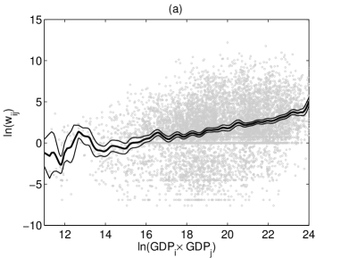
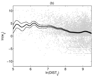
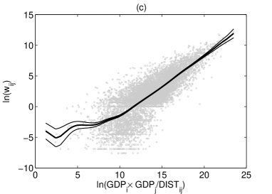
Furthermore, a gravity-law structure clearly emerges if one studies how bilateral trade flows correlate with the product of ’s and ’s GDPs and their geographical distance. Figure 1 plots in a log-log scale against , and . Non-parametric estimates of conditional means, superimposed on the clouds of points together with %95 confidence bounds, clearly indicate that both the correlation structure and the functional form linking to size and geographical effects are in line with the prediction of the basic gravity law 555Conditional means have been estimated using the local-linear non-parametric method proposed in Ref. (Li and Racine, 2004), employing cross-validated bandwidth selection using the procedure of Ref. (Hurvich et al., 1998). Estimation has been performed using the package np (Hayfield and Racine, 2008) under R (http://www.r-project.org/)..
From an empirical perspective, the basic gravity equation has been expanded in the literature to improve the fit by taking into account country- or trade-specific characteristics that may influence bilateral trade flows in addition to masses and distance (see previous section). Overall, this strategy has proven itself to be extremely successful in order to explore the determinants of bilateral trade flows and we shall replicate it in what follows 666On this huge empirical literature, see for example Refs. (Overman et al., 2003; Frankel, 1997; Rose and Spiegel, 2002; Rose, 2000; Glick and Rose, 2001; Eichengreen and Irwin, 1996; Leamer and Levinsohn, 1995; Feenstra et al., 2001), among others..
For our estimation purposes, it is convenient to start with the most general multiplicative formulation of the gravity equation (Santos Silva and Tenreyro, 2006), which reads:
| (1) | |||
Here (with ) is the -dimensional vector of symmetric bilateral trade flows (i.e. the upper-diagonal entries of the weight matrix ); are unknown (vectors of) parameters to be estimated; are - dimensional vectors of country-specific continuous or categorical variables (other than GDP); are -dimensional vectors of country-specific dummy variables; are -dimensional vectors of link-specific dummy variables (other than distance); are country-specific fixed effects (see below); and is an error term, statistically independent on the regressors, s.t. its mean conditional on all regressors is equal to 1. In our exercises below, =(AREA, POP, CPI, EXC, RM), =(LL, CONT), whereas =(CTG, COMC, COML, COL, TA, COMR), see Appendix B.
The estimation of eq. (1) is not easy and it potentially entails many difficulties. Among them, we recall the treatment of zero-valued flows (Santos Silva and Tenreyro, 2006; Linders and de Groot, 2006; Burger et al., 2009), non-linearity and heteroscedasticity (Santos Silva and Tenreyro, 2006), endogeneity and omitted-term biases (Baldwin and Taglioni, 2006). In order to simultaneously deal with all these problems, we estimate Eq. (1) using a zero-inflated Poisson pseudo-maximum likelihood (ZIPPML) model (Burger et al., 2009) with country-fixed effects (Baldwin and Taglioni, 2006) to overcome endogeneity due to omitted terms (e.g., related to non-observable variables as landed prices of origin goods in destination country, which may in principle be correlated with trade-cost terms, as proxied by distance) 777Note that all variables have been original deflated, but this does not create any difficulty here as we undertake a cross-section study.. To double-check our results, we also estimate Eq. (1) with alternative econometric approaches discussed in the relevant literature (Linders and de Groot, 2006), including standard OLS on the log-linearized form (omitting zero-valued flows or substituting zero-valued flows by a small constant), log-normal pseudo-maximum likelihood estimators as in Ref. (Santos Silva and Tenreyro, 2006), and zero-inflated negative-binomial pseudo-maximum likelihood (ZINBMML) techniques (Burger et al., 2009). Overall, we obtain the best fit using the ZIPPML estimator, although our results are not dramatically different under alternative estimation strategies, both in terms of model selection and correlation of residuals, a tendency already documented in Ref. (Linders and de Groot, 2006).
— TABLE 2 ABOUT HERE —
Table 2 reports the ZIPPML fit to year-2000 data, together with usual goodness-of-fit statistics 888The ZIPPML is a two-stage procedure (Wooldridge, 2001). The first stage features a logit regression estimating the probability that there is no bilateral trade at all. In the second stage, a Poisson regression is run to fit trade flows of the non-zero group of link (as estimated in the first stage). We use the same regressors (Appendix B) to model both the first and second stage. Here we show only the estimation results for the Poisson final stage for the sake of exposition (the complete set of regression results is available on request from the Author). All exercises have been performed using Stata 9 (StataCorp, 2007).. The final model has been selected by successively removing the regressors that were not contributing a significant impact on the overall likelihood, using a general-to-specific procedure. Only GDP, DIST, AREA, POP, LL, CTG, COML, COL, TA resisted this successive selection. The final gravity equation seems well-specified, according to both Wald (Wooldridge, 2001) and Vuong (Vuong, 1989) test statistics, and achieves an extremely large adjusted (0.93) —a typical performance of trade gravity equations. All signs and magnitudes of estimated coefficients are in line with those found in the relevant literature. Trade flows are positively affected by country GDP, existence of trade agreements, common borders, common language and colony relationships. They are negatively affected by distance, area and population (net of GDP effects), as well as the probability of being landlocked. Country remoteness, continental position, religion, exchange rates and CPI-effects do not appear instead to significantly affect trade flows in our data.
Define as the estimated residual from eq. (1), i.e. obtained by substituting unknown parameters with estimated ones from Table 2. Note that can be interpreted as the weight of the trade link once all structural effects related to country size, geographical, social, historical and political factors have been removed from the original weight . It is then straightforward to define the “residual” weighted ITN by simply re-weight links using the s 999See Ref. (Krempel and Pluemper, 2003) for a germane approach aimed at visualizing the properties of the ITN.. In what follows, we will then study the topological properties of the residual symmetric weight matrix , where for , for , and for all , and compare them with those of .
IV Topological Properties of Gravity-Equation Residual Networks
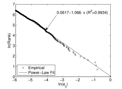
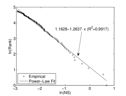
One of the most puzzling stylized facts emerging from the study of the topological properties of is that the distribution of link weights is well approximated by a log-normal density (Li et al., 2003; Fagiolo et al., 2009a). Indeed, this militates against the view that the ITN is a complex network, as log-normality can be simply the limit outcome of uncorrelated link-weight multiplicative growth processes (e.g., Gibrat laws; see Ref. (Sutton, 1997)). In other words, original link weights are markedly heterogeneous but display exponentially-decaying upper tails, without the typical fat-tailed behavior that is known to be the signature of complexity (Mitzenmacher, 2004; Rosser, 2008). The present analysis shows that, once all gravity-equation dependence is removed from the original data, the residual ITN is characterized by power-law distributed link weights, see the size-rank plot (Stanley et al., 1995) in Figure 3. In fact, the correlation between original and residual weights is not statistically-significantly different from zero (-0.009, with a p-value 0.9171). We shall go back to the implications of this finding on modeling below. For the moment, let us stress the fact that power-law behavior of residual link weights hints to an inherent complex behavior of trade flows, possibly due to deep similarities between countries, which are somewhat hidden by the standard determinants of trade accounted for in the empirical literature.
We now explore how the other topological properties of the residual ITN compare to original ones. As it is customary in this literature, we shall focus on node strength (NS), defined as the sum of all link weights of a node; node average nearest-neighbor strength (ANNS), i.e. the average strength of the trade partners of that node; weighted node-clustering (WCC), measured as the relative weighted intensity of trade triangles with that node as one of the vertices; and random-walk betweenness centrality (RWBC), accounting for global centrality of a node in the weighted network 101010See Appendix C for formal definitions. Notice also that the ZIPPML estimator seems to consistently predict the density of the residual ITN. Indeed, the fraction of all possible links with positive weight is 0.63 under and 0.62 in the residual graph ..
As happens for link weights, power-law shapes characterize in the residual ITN all node statistics (NS, ANNS, and WCC) that were originally well-proxied by log-normal densities (Fagiolo et al., 2009a), see Figure 3 for NS. Interestingly, the only topological property that was power-law shaped in the original ITN (RWBC) keeps the same shape also in the residual network. RWBC is actually a peculiar statistics, because, unlike the others, each of its node values somewhat reflect the whole structure of the network. The fact that RWBC is still power-law distributed suggests that complexity is really an intrinsic feature of the ITN.
— TABLE 3 ABOUT HERE —
Another robust set of stylized facts regarding the weighted ITN concerns the correlation structure among node-distributions of topological statistics, and between node topological statistics and country per-capita GDP (as a proxy for country income). Table 3 reports such a correlation structure for both the original ITN () and the residual one (). Coefficients not statistically-significantly different from zero are marked in boldface. The original ITN, where all correlation coefficients were statistically different from zero, hinted to a trade structure where countries that trade more intensively are also high-income ones, they are more clustered and central, but tend to trade with relatively-less connected partners. This configures a relatively disassortative pattern for the ITN. Once size, geographically-related and other determinants of trade have been removed from the data, however, the topological properties of the residual ITN are almost uncorrelated with their original counterpart. The only exception is ANNS, which displays a strong and negative correlation. This suggests that countries that in typically traded with intensively connected partners (i.e., small and poor countries) exhibit in small ANNS values, i.e. tend to trade with poorly-connected partners, a pattern that can be intuitively explained by recalling that trade flows in do not reflect any size, geographic, or colonial preferential relationship. Note also that in countries that trade more intensively (i.e., high NS) still are more central and clustered, but do not display any assortative or disassortative pattern anymore, as the NS-ANNS correlation in is not significantly-different from zero. Furthermore, the removal of size effects (GDP and population) naturally destroys any positive correlation between income and trade intensity, centrality and clustering: now high-income countries tend to trade relatively less intensively and occupy less central positions (and trade with relatively more connected partners).
This result is confirmed by looking at the Spearman’s rank-correlation coefficient between country-statistic rankings. If one correlates, e.g., the rank of countries under and according to node statistics, it emerges that rankings made with respect to NS, WCC and RWBC are only weakly (positively) correlated, whereas the correlation for ANNS rankings is equal to -0.7676. This suggests that if a country was scoring high in terms of intensity of trade (NS), clustering (WCC) and centrality (RWBC) in the original ITN, it is not likely to keep its top position in the residual network, and with high probability will appear at the bottom of the list in the ANNS ranking, see Figure 4. For example, whereas the US, Germany and Japan used to occupy top positions in the rankings of trade intensity, clustering and centrality, in the residual network such positions are now filled by relatively small but very dynamic countries like Iceland, Korea, Belgium, as well as middle-east oil-related countries (United-Arab Emirates) and many African ones. Furthermore, the ANNS ranking, which was topped in by micro-economies (e.g., Pacific islanders) now features in the first positions relatively large and active countries (Cameroon, Senegal, Kenya, Rumania, Colombia, Morocco, South Africa, Mexico), as well as China and Indonesia.
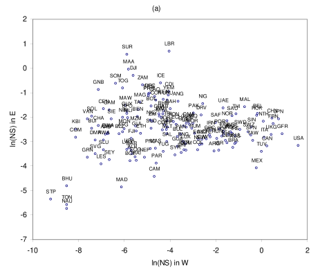
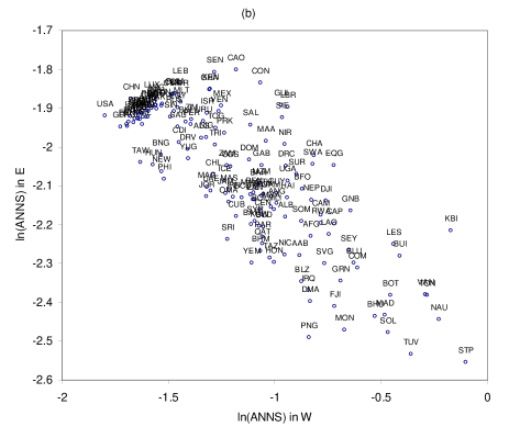
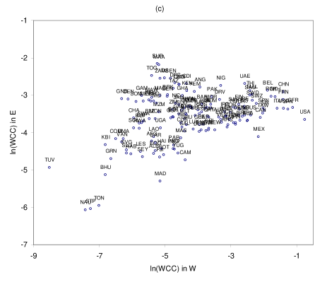
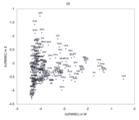
All in all, the foregoing analysis shows that only few of the stylized facts found for the weighted ITN apply to its residual version, and that a great extent of ITN topological features can be explained by the control variables employed in the gravity-equation regression. Our results also indicate that, removing such structure from the data and interpreting residuals as proxies for the underlying trade similarities between countries, interesting patterns emerge about the inherent complex structure of the ITN and how countries are interconnected and play their roles in the network.
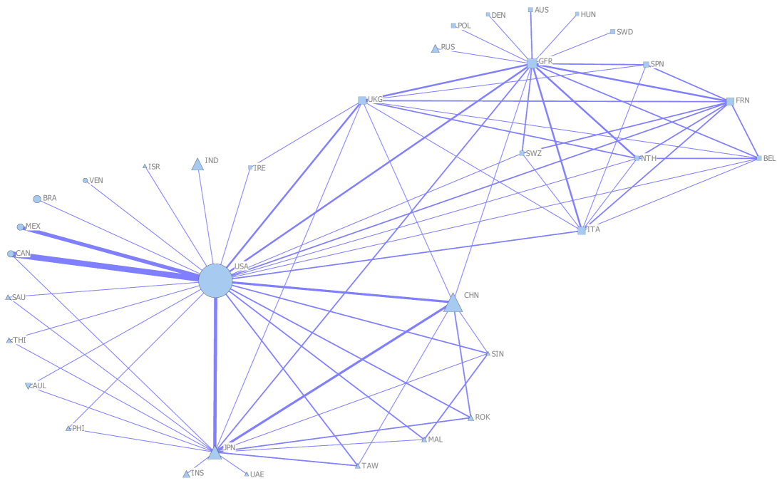
Additional insights on these relationships can be gathered from a simple weighted-graph visualization of the original vs. residual ITN. Figures 5-6 depict a partial view (largest 1% links in terms of weights) of the original and residual ITN in year 2000 as an undirected graph where the thickness of a link is proportional to its weight, node size is proportional to country’s GDP, and node shapes represent the continent which the country belongs to. It is easy to see that, as discussed in the previous sections, large countries tend to trade more intensively with each other, with contiguous/close countries or with partners that are relevant in terms of history and trade agreements. The original ITN is also characterized by a core-periphery structure where large influential countries (USA, Japan, China, Germany, France, Italy, etc.) play the role of hubs, attached to many other countries by relatively weaker trade links. Geographical clustering is also evident, as same-continent countries tend to be tightly interconnected.
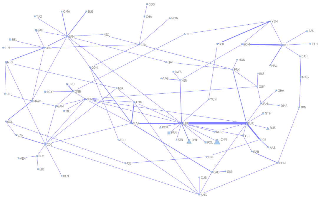
Simple inspection of the residual weighted ITN graph (links with largest 1% of weight in ) hints instead to a much more interconnected pattern, characterized by much more spread links, without large-sized hubs, nor excessive geographical clustering. All large-GDP countries disappear from the graph (e.g., USA, Germany, Italy, France). Small and medium-sized African, South-American and Asian countries are most represented, possibly because of their endowments in tradable natural resources and/or over-specialization of their export profile.
Some countries, like Liberia, Surinam, Mauritania and Djibuti, play an unexpectedly prominent role in the network. These are countries with relatively low per-capita GDPs, which in the original network were holding many trade relationships (between 52 and 88) and scored around the median in all node-statistic rankings (except centrality). The majority of their trade relationships were weak but occurred outside trade agreements. Unlike Pacific islanders, such flows did not necessarily concern large-sized partners, were not related to colony relationships and not necessarily geographically close (they are not landlocked). Therefore, it is not a surprise that their residual link weights end up being relatively large for many existing relationships, thus promoting such countries to more important positions in the network.
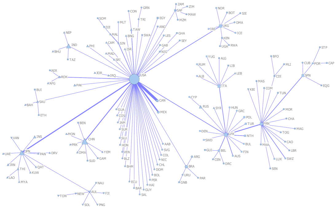
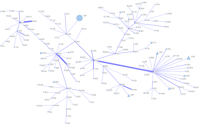
Finally, to get a more precise feeling of the role of large-sized countries in the residual network, we plot the complete minimal spanning trees (MSTs) associated to and 111111See Ref. (Gower and Ross, 1969). To build the MST of a weighted graph with link-weights in the unit interval we have employed the following procedure. First, assume that information from link weights can be treated the same way as correlation coefficients in Ref. (Mantegna, 1999), i.e. that higher (symmetric) link weights signal a higher trade similarity between countries. Second, transform weight (i.e., similarity) matrices entries and into, respectively, and , and let . As explained in Ref. (Mantegna, 1999), this is an appropriate metric distance. Third, we have computed the MST associated to and , and re-scaled the link weights returned by the Kruskal’s algorithm (Cormen et al., 2001, Ch. 23.2) by their maximum values, in line with what we have done for and . Finally, we have weighted any resulting link by and , to get the right proportionality between weights and similarity.. This graphical analysis may complement the former because, by simplifying the structure of the network, allows one to simultaneously visualize all existing nodes and their relevant interactions, a thing that was simply impossible to do with and , given the extremely large density of the two graphs. The plot of -MST (Figure 7) magnifies the hub-role of the largest countries, especially the US, and better accounts for the position of other peripheral countries in the ITN. Conversely, the plot of -MST (Figure 8) hints to a relatively more central role of very small countries like Liberia and Surinam (see above); downplays the importance of hubs and geography; and relegates large countries at the periphery. For instance, US and China now link to small countries in the ITN, whereas India keeps having a marginal position.
V Conclusions
In this paper we have begun to investigate the determinants of the statistical features of the weighted international-trade network. We have compared the topological properties of the ITN, as originally explored in a series of papers (Li et al., 2003; Bhattacharya et al., 2008, 2007; Garlaschelli et al., 2007; Fagiolo et al., 2008; Fagiolo et al., 2009a), to those of the residual weighted symmetric ITN. The latter has been obtained after fitting original bilateral-trade flows via a standard gravity equation including as regressors country GDP, population and area; geographical distance between countries; and a series of link- or country-specific variables accounting for other factors related to geography (common border, landlocking, continent), the economy (trade agreements, exchange rates, consumer price indices), and social/ political/ historical effects (common language, religion, and currency).
Our findings indicate that the residual ITN is characterized by power-law shaped distributions of link weights and node statistics (e.g., strength, clustering, random-walk betweenness centrality). Hence, the underlying architecture of the weighted ITN seems to exhibit signatures of complexity, unlike its original counterpart. We have also found that the correlation structure among node statistics, and between node statistics and country per-capita GDP, changes substantially when comparing the original and residual weighted networks. Whereas the original ITN displays a structure with a few large-sized country hubs and a relatively strong connectivity among nearby countries (either geographically, socially, politically or economically), the residual ITN is organized around many relatively small-sized but trade-oriented countries that, independently of their geographical position, either play the role of local hubs or attract large and rich countries in complex trade-interaction patterns.
Our results have some implications for modeling purposes. Indeed, the strong gravity-like dependence that, in line with existing literature, can be detected in ITN data, as well as the impact of removing such structure on ITN topological properties, suggests that any model of network formation and link-weight evolution aiming at replicating ITN topological properties should consider country size, geography, etc. among its building blocks. This may occur, for instance, by devising dynamic models of network formation and weight evolution where node size and position, contiguity and agreements, matter in the decision of the nodes to form/delete a link, or to change its weight. At the same time, models aiming at explaining and replicating ITN stylized facts should allow empirical calibration of their node- and link-related characteristics (see, Refs. (Garlaschelli and Loffredo, 2004, 2005; Garlaschelli et al., 2007; Bhattacharya et al., 2008) for preliminary exercises in this direction). This may be relevant for predictive and policy exercises. Furthermore, our findings call for models that are simultaneously able to replicate the set of stylized facts of both the original and the residual ITN (no matter the determinants accounted for in the gravity equation). For example, it would be important to have models of the ITN that recover log-normality of the (equilibrium) link-weight distribution when size and geography are not accounted for, and power-law shapes after having controlled for them.
To conclude, it may be worthwhile to notice that the simple and preliminary exercises described in this article may be extended in at least two directions. First, one may take a specific-to-general approach to gravity-equation modeling, and adding an increasing number of factors in its specification. For example, one may begin with size only, and gradually introduce geography, trade agreements, etc.. At each step a residual ITN can be defined and its properties can be accordingly compared to those of the original ITN. This analysis may end up in a minimal “sufficient” set of determinants able to, e.g., account for a complex ITN structure, or changes in node-statistics correlation patterns. Finally, one might play with expanded versions of the gravity equation that consider, e.g., country-specific natural endowments, industrial profile and trade specialization. This might shed some light on the peculiar structure of the residual network and explain trade patterns that otherwise could remain obscure.
References
- Li et al. (2003) X. Li, Y. Y. Jin, and G. Chen, Physica A: Statistical Mechanics and its Applications 328, 287 (2003).
- Serrano and Boguñá (2003) A. Serrano and M. Boguñá, Physical Review E 68, 015101(R) (2003).
- Garlaschelli and Loffredo (2004) D. Garlaschelli and M. Loffredo, Physical Review Letters 93, 188701 (2004).
- Garlaschelli and Loffredo (2005) D. Garlaschelli and M. Loffredo, Physica A 355, 138 (2005).
- Serrano et al. (2007) A. Serrano, M. Boguñá, and A. Vespignani, Journal of Economic Interaction and Coordination 2, 111 (2007).
- Bhattacharya et al. (2008) K. Bhattacharya, G. Mukherjee, J. Sarämaki, K. Kaski, and S. Manna, Journal of Statistical Mechanics: Theory Exp. A 2, P02002 (2008).
- Bhattacharya et al. (2007) K. Bhattacharya, G. Mukherjee, and S. Manna, in Econophysics of Markets and Business Networks, edited by A. Chatterjee and B. Chakrabarti (Springer-Verlag, Milan, Italy, 2007).
- Garlaschelli et al. (2007) D. Garlaschelli, T. Di Matteo, T. Aste, G. Caldarelli, and M. Loffredo, The European Physical Journal B 57, 1434 (2007).
- Tzekina et al. (2008) I. Tzekina, K. Danthi, and D. Rockmore, The European Physical Journal B - Condensed Matter 63, 541 (2008).
- Fagiolo et al. (2008) G. Fagiolo, S. Schiavo, and J. Reyes, Physica A 387, 3868 (2008).
- Reyes et al. (2008) J. Reyes, S. Schiavo, and G. Fagiolo, Advances in Complex Systems 11, 685 (2008).
- Fagiolo et al. (2009a) G. Fagiolo, S. Schiavo, and J. Reyes, Physical Review E 79, 036115 (2009a).
- Reichardt and White (2007) J. Reichardt and D. White, The European Physical Journal B 60, 217 (2007).
- Helliwell and Padmore (1985) J. F. Helliwell and T. Padmore, in Handbook of International Economies, edited by R. Jones and P. Kenen (Elsevier Science Publishers B.V., 1985).
- Artis et al. (2003) M. Artis, A.-B. Galvão, and M. Marcellino, Economics Working Papers ECO2003/18, European University Institute (2003).
- Forbes (2002) K. Forbes, in Preventing Currency Crises in Emerging Markets, edited by E. Sebastian and F. Jeffrey (Chicago, University of Chicago Press, 2002).
- Krugman (1995) P. Krugman, Brookings Papers on Economic Activity 26, 327 (1995).
- Abeysinghe and Forbes (2005) T. Abeysinghe and K. Forbes, Review of International Economics 13, 356 (2005).
- Albert and Barabási (2002) R. Albert and A.-L. Barabási, Reviews of Modern Physics 74, 47 (2002).
- Dorogovtsev and Mendes (2003) S. Dorogovtsev and J. Mendes, Evolution of Networks: From Biological Nets to the Internet and WWW (Oxford, Oxford University Press, 2003).
- Kali and Reyes (2007) R. Kali and J. Reyes, Journal of International Business Studies 38, 595 (2007).
- Kali et al. (2007) R. Kali, F. Méndez, and J. Reyes, Journal of International Trade & Economic Development 16, 245 (2007).
- Barrat et al. (2004) A. Barrat, M. Barthélemy, R. Pastor-Satorras, and A. Vespignani, Proceedings of the National Academy of Sciences 101, 3747 (2004).
- Barthélemy et al. (2005) M. Barthélemy, A. Barrat, R. Pastor-Satorras, and A. Vespignani, Physica A 346, 34 (2005).
- Jackson et al. (2003) M. O. Jackson, G. Demange, S. Goyal, and A. V. D. Nouwel, in In Group Formation in Economics: Networks, Clubs and Coalitions (Cambridge University Press, 2003).
- Leamer and Levinsohn (1995) E. E. Leamer and J. Levinsohn, in Handbook of International Economics, edited by G. M. Grossman and K. Rogoff (Elsevier, 1995), vol. 3 of Handbook of International Economics, chap. 26, pp. 1339–1394.
- Overman et al. (2003) H. G. Overman, S. Redding, and A. J. Venables, in Handbook of International Trade, edited by J. Harrigan and K. Choi (Blackwell Publishers, 2003), pp. 353–387.
- Fagiolo (2007) G. Fagiolo, Physical Review E 76, 026107 (2007).
- Fagiolo et al. (2009b) G. Fagiolo, S. Schiavo, and J. Reyes, Journal of Evolutionary Economics (2009b), forthcoming.
- Gleditsch (2002) K. Gleditsch, Journal of Conflict Resolution 46, 712 (2002).
- Bhavnani et al. (2002) R. Bhavnani, D. T. Coe, A. Subramanian, and N. T. Tamirisa, IMF Working Papers 02/171, International Monetary Fund (2002).
- Fratianni (2009) M. Fratianni, in The Oxford Handbook of International Business, edited by A. M. Rugman (Oxford University Press, Oxford, U.K., 2009).
- Santos Silva and Tenreyro (2006) J. M. C. Santos Silva and S. Tenreyro, The Review of Economics and Statistics 88, 641 (2006).
- Linders and de Groot (2006) G.-J. M. Linders and H. L. de Groot, Tinbergen Institute Discussion Papers 06-072/3, Tinbergen Institute (2006).
- Burger et al. (2009) M. Burger, F. v. Oort, and G. Linders, Research Paper ERS-2009-003-ORG Revision, Erasmus Research Institute of Management (ERIM) (2009).
- Baldwin and Taglioni (2006) R. Baldwin and D. Taglioni, NBER Working Papers 12516, National Bureau of Economic Research (2006).
- Wooldridge (2001) J. M. Wooldridge, Econometric Analysis of Cross Section and Panel Data (Boston, The MIT Press, 2001).
- Vuong (1989) Q. H. Vuong, Econometrica 57, 307 (1989).
- Sutton (1997) J. Sutton, Journal of Economic Literature 35, 40 (1997).
- Mitzenmacher (2004) M. Mitzenmacher, Internet Mathematics 1, 226 (2004).
- Rosser (2008) J. B. Rosser, Advances in Complex Systems (ACS) 11, 745 (2008).
- Stanley et al. (1995) M. H. R. Stanley, S. V. Buldyrev, S. Havlin, R. N. Mantegna, M. A. Salinger, and H. Eugene Stanley, Economics Letters 49, 453 (1995).
- Anderson (1979) J. E. Anderson, American Economic Review 69, 106 (1979).
- Bergstrand (1985) J. H. Bergstrand, The Review of Economics and Statistics 67, 474 (1985).
- Deardorff (1998) A. Deardorff, in The Regionalization of the World Economy (National Bureau of Economic Research, 1998), NBER Chapters, pp. 7–32.
- Anderson and van Wincoop (2003) J. E. Anderson and E. van Wincoop, American Economic Review 93, 170 (2003).
- Li and Racine (2004) Q. Li and J. Racine, Statistica Sinica 14, 485 512 (2004).
- Hurvich et al. (1998) C. Hurvich, J. Simonoff, and C. Tsai, Journal of the Royal Statistical Society Series B 60, 271 293 (1998).
- Hayfield and Racine (2008) T. Hayfield and J. S. Racine, Journal of Statistical Software 27 (2008).
- Glick and Rose (2001) R. Glick and A. K. Rose, NBER Working Papers 8396, National Bureau of Economic Research (2001).
- Rose and Spiegel (2002) A. K. Rose and M. M. Spiegel, Working Papers in Applied Economic Theory 2002–09, Federal Reserve Bank of San Francisco (2002).
- Frankel (1997) J. Frankel, Regional Trading Blocs in the World Economic System (Institute for International Economics, 1997).
- Rose (2000) A. K. Rose, Economic Policy 30, 9 (2000).
- Eichengreen and Irwin (1996) B. Eichengreen and D. A. Irwin, NBER Working Papers 5565, National Bureau of Economic Research (1996).
- Feenstra et al. (2001) R. C. Feenstra, J. R. Markusen, and A. K. Rose, Canadian Journal of Economics 34, 430 (2001).
- StataCorp (2007) StataCorp, Stata Statistical Software: Release 10 (College Station, TX: StataCorp LP, 2007).
- Krempel and Pluemper (2003) L. Krempel and T. Pluemper, Journal of Social Structure 4, 1 (2003).
- Gower and Ross (1969) J. C. Gower and G. J. S. Ross, Applied Statistics 18, 54 (1969).
- Mantegna (1999) R. Mantegna, The European Physical Journal B 11, 193 (1999).
- Cormen et al. (2001) T. H. Cormen, C. E. Leiserson, R. L. Rivest, and C. Stein, Introduction to Algorithms (MIT Press and McGraw-Hill, 2001).
- DeMontis et al. (2005) A. DeMontis, M. Barthélemy, A. Chessa, and A. Vespignani, Environment And Planning B - Planning and Design 34, 905 (2005).
- Saramaki et al. (2007) J. Saramaki, M. Kivelä, J. Onnela, K. Kaski, and J. Kertész, Physical Review E 75, 027105 (2007).
- Watts and Strogatz (1998) D. Watts and S. Strogatz, Nature 393, 440 (1998).
- Newman (2005) M. Newman, Social Networks 27, 39 (2005).
- Fisher and Vega-Redondo (2006) E. Fisher and F. Vega-Redondo, Working Paper, Cal Poly (2006).
Appendix A List of Countries in the Balanced Panel (1981-2000).
| ID | Acro | Name | ID | Acro | Name | ID | Acro | Name |
|---|---|---|---|---|---|---|---|---|
| 2 | USA | United States | 355 | BUL | Bulgaria | 600 | MOR | Morocco |
| 20 | CAN | Canada | 360 | RUM | Rumania | 615 | ALG | Algeria |
| 31 | BHM | Bahamas | 365 | RUS | Russia | 616 | TUN | Tunisia |
| 40 | CUB | Cuba | 375 | FIN | Finland | 620 | LIB | Libya |
| 41 | HAI | Haiti | 380 | SWD | Sweden | 625 | SUD | Sudan |
| 42 | DOM | Dominican Rep. | 385 | NOR | Norway | 630 | IRN | Iran |
| 51 | JAM | Jamaica | 390 | DEN | Denmark | 640 | TUR | Turkey |
| 52 | TRI | Trinidad/Tobago | 395 | ICE | Iceland | 645 | IRQ | Iraq |
| 53 | BAR | Barbados | 402 | CAP | Cape Verde | 651 | EGY | Egypt |
| 54 | DMA | Dominica | 403 | STP | Sao Tome | 652 | SYR | Syria |
| 55 | GRN | Grenada | 404 | GNB | Guinea-Bissau | 660 | LEB | Lebanon |
| 56 | SLU | Saint Lucia | 411 | EQG | Eq. Guinea | 663 | JOR | Jordan |
| 57 | SVG | St. Vincent | 420 | GAM | Gambia | 666 | ISR | Israel |
| 58 | AAB | Antigua | 432 | MLI | Mali | 670 | SAU | Saudi Arabia |
| 70 | MEX | Mexico | 433 | SEN | Senegal | 678 | YEM | Yemen |
| 80 | BLZ | Belize | 434 | BEN | Benin | 690 | KUW | Kuwait |
| 90 | GUA | Guatemala | 435 | MAA | Mauritania | 692 | BAH | Bahrain |
| 91 | HON | Honduras | 436 | NIR | Niger | 694 | QAT | Qatar |
| 92 | SAL | El Salvador | 437 | CDI | Cote D Ivoire | 696 | UAE | Arab Emirates |
| 93 | NIC | Nicaragua | 438 | GUI | Guinea | 698 | OMA | Oman |
| 94 | COS | Costa Rica | 439 | BFO | Burkina Faso | 700 | AFG | Afghanistan |
| 95 | PAN | Panama | 450 | LBR | Liberia | 710 | CHN | China |
| 100 | COL | Colombia | 451 | SIE | Sierra Leone | 712 | MON | Mongolia |
| 101 | VEN | Venezuela | 452 | GHA | Ghana | 713 | TAW | Taiwan |
| 110 | GUY | Guyana | 461 | TOG | Togo | 731 | PRK | North Korea |
| 115 | SUR | Surinam | 471 | CAO | Cameroon | 732 | ROK | South Korea |
| 130 | ECU | Ecuador | 475 | NIG | Nigeria | 740 | JPN | Japan |
| 135 | PER | Peru | 481 | GAB | Gabon | 750 | IND | India |
| 140 | BRA | Brazil | 482 | CEN | Centr African Rep. | 760 | BHU | Bhutan |
| 145 | BOL | Bolivia | 483 | CHA | Chad | 770 | PAK | Pakistan |
| 150 | PAR | Paraguay | 484 | CON | Congo | 771 | BNG | Bangladesh |
| 155 | CHL | Chile | 490 | DRC | Congo (Zaire) | 775 | MYA | Myanmar |
| 160 | ARG | Argentina | 500 | UGA | Uganda | 780 | SRI | Sri Lanka |
| 165 | URU | Uruguay | 501 | KEN | Kenya | 781 | MAD | Maldives |
| 200 | UKG | United Kingdom | 510 | TAZ | Tanzania | 790 | NEP | Nepal |
| 205 | IRE | Ireland | 516 | BUI | Burundi | 800 | THI | Thailand |
| 210 | NTH | Netherlands | 517 | RWA | Rwanda | 811 | CAM | Cambodia |
| 211 | BEL | Belgium | 520 | SOM | Somalia | 812 | LAO | Laos |
| 212 | LUX | Luxembourg | 522 | DJI | Djibouti | 816 | DRV | Vietnam |
| 220 | FRN | France | 530 | ETH | Ethiopia | 820 | MAL | Malaysia |
| 225 | SWZ | Switzerland | 540 | ANG | Angola | 830 | SIN | Singapore |
| 230 | SPN | Spain | 541 | MZM | Mozambique | 840 | PHI | Philippines |
| 235 | POR | Portugal | 551 | ZAM | Zambia | 850 | INS | Indonesia |
| 260 | GFR | Germany | 552 | ZIM | Zimbabwe | 900 | AUL | Australia |
| 290 | POL | Poland | 553 | MAW | Malawi | 910 | PNG | Papua |
| 305 | AUS | Austria | 560 | SAF | South Africa | 920 | NEW | New Zealand |
| 310 | HUN | Hungary | 570 | LES | Lesotho | 935 | VAN | Vanuatu |
| 325 | ITA | Italy | 571 | BOT | Botswana | 940 | SOL | Solomon’s |
| 338 | MLT | Malta | 572 | SWA | Swaziland | 950 | FJI | Fiji |
| 339 | ALB | Albania | 580 | MAG | Madagascar | 970 | KBI | Kiribati |
| 345 | YUG | Yugoslavia | 581 | COM | Comoros | 971 | NAU | Nauru |
| 350 | GRC | Greece | 590 | MAS | Mauritius | 972 | TON | Tonga |
| 352 | CYP | Cyprus | 591 | SEY | Seychelles | 973 | TUV | Tuvalu |
Appendix B List of link- or country-related additional variables employed in gravity-equation exercises.
| Label | Related to | Explanation | Source |
|---|---|---|---|
| GDP | Country | Gross-domestic product | Gleditsch (2002) |
| AREA | Country | Country area in Km2 | CEPII (http://www.cepii.fr/) |
| POP | Country | Country population | Gleditsch (2002) |
| LL | Country | Dummy variable equal to 1 for landlocked countries | CEPII (http://www.cepii.fr/) |
| CONT | Country | Dummy variables recording the continent to which the country belongs | CEPII (http://www.cepii.fr/) |
| RM | Country | Country remoteness index defined as the weighted average of the distances of a country to all other countries, with weights equal to the country share of world GDP, see (Bhavnani et al., 2002). | Our computations on CEPII and Gleditsch (200) data |
| CPI | Country | Consumer price index | International Monetary Fund (www.imf.org) |
| DIST | Link | Geodesic geographical distance between two countries, calculated with the great circle formula | CEPII (http://www.cepii.fr/) |
| CTG | Link | Contiguity dummy equal to 1 if two countries share a common border | CEPII (http://www.cepii.fr/) |
| COMC | Link | Dummy equal to 1 if two countries use the same currency | Our computation on Andrew Rose dataset (http://faculty.haas.berkeley.edu/arose), see also (Glick and Rose, 2001). |
| COML | Link | Dummy equal to 1 if the official language (or mother tongue or second language) of the two countries is the same | CEPII (http://www.cepii.fr/) |
| COL | Link | Dummy equal to 1 if the two countries share a substantial colonizer-colonized relationship | CEPII (http://www.cepii.fr/) |
| TA | Link | Dummy variable equal to 1 for countries involved in regional, bilateral or preferential trade agreements in year 1995 still in place in year 2000 | WTO (http://www.wto.org/) |
| EXC | Link | Nominal exchange rates | International Monetary Fund (www.imf.org) |
| COMR | Link | Dummy equal to 1 if the two countries share a common religion | Our computations on Andrew Rose dataset (http://faculty.haas.berkeley.edu/arose), see also (Rose and Spiegel, 2002). |
Appendix C Network Statistics
Given a symmetric weight matrix , with , define the associated symmetric adjacency matrix as , where iff and zero otherwise. In the paper, we make use of the following statistics:
-
•
Node degree (Albert and Barabási, 2002), defined as , where is the -th row of and 1 is a unary vector. ND is a measure of binary connectivity, as it counts the number of trade partners of any given node. Although we mainly focus here on a weighted-network approach, we study ND because of its natural interpretation in terms of number of trade partnerships and bilateral trade agreements.
-
•
Node strength (DeMontis et al., 2005), defined as , where is the -th row of . NS is a measure of weighted connectivity, as it gives us an idea of how intense existing trade relationships of country are.
-
•
Node average nearest-neighbor strength (DeMontis et al., 2005), that is . ANNS measures how intense are trade relationships maintained by the partners of a given node. Therefore, the correlation between ANNS and NS is a measure of network assortativity (if positive) or disassortativity (if negative).
-
•
Weighted clustering coefficient (Saramaki et al., 2007; Fagiolo, 2007), defined as
Here is the -th entry on the main diagonal of and stands for the matrix obtained from after raising each entry to . WCC measures how much clustered a node is from a weighted perspective, i.e. how much intense are the linkages of trade triangles having country as a vertex. Replacing with , one obtains the standard binary clustering coefficient (BCC), which counts the fraction of triangles existing in the neighborhood of any give node (Watts and Strogatz, 1998).
-
•
Random-walk betweenness centrality (Newman, 2005; Fisher and Vega-Redondo, 2006), which is a measure of how much a given country is globally-central in the ITN. A node has a higher random-walk betweenness centrality (RWBC) the more it has a position of strategic significance in the overall structure of the network. In other words, RWBC is the extension of node betweenness centrality to weighted networks and measures the probability that a random signal can find its way through the network and reach the target node where the links to follow are chosen with a probability proportional to their weights.
| % Total | |||||||||||||
|---|---|---|---|---|---|---|---|---|---|---|---|---|---|
| N America | C America | S America | Cont Europe | East Europe | Middle East | C Asia | China & E Asia | N Africa | C Africa | S Africa | Pacific | Trade | |
| N America | 31.87% | 12.35% | 3.66% | 18.52% | 0.71% | 2.68% | 0.98% | 26.57% | 0.44% | 0.68% | 0.49% | 1.05% | 20.49% |
| C America | 74.19% | 3.96% | 3.37% | 8.50% | 0.44% | 0.59% | 0.15% | 8.06% | 0.15% | 0.15% | 0.15% | 0.29% | 3.41% |
| S America | 29.88% | 4.58% | 23.90% | 22.11% | 1.00% | 1.99% | 0.80% | 12.35% | 1.20% | 1.00% | 0.60% | 0.60% | 2.51% |
| Cont Europe | 9.75% | 0.75% | 1.43% | 67.53% | 3.75% | 3.17% | 0.76% | 9.44% | 1.45% | 0.72% | 0.64% | 0.60% | 38.91% |
| East Europe | 6.43% | 0.67% | 1.11% | 64.75% | 10.64% | 3.99% | 0.89% | 9.76% | 0.67% | 0.67% | 0.22% | 0.22% | 2.26% |
| Middle East | 13.87% | 0.50% | 1.26% | 31.15% | 2.27% | 9.08% | 4.67% | 32.53% | 1.51% | 0.63% | 1.26% | 1.26% | 3.97% |
| C Asia | 16.53% | 0.41% | 1.65% | 24.38% | 1.65% | 15.29% | 4.55% | 29.34% | 1.24% | 2.48% | 0.83% | 1.65% | 1.21% |
| China & E Asia | 23.08% | 1.17% | 1.31% | 15.58% | 0.93% | 5.47% | 1.50% | 46.82% | 0.32% | 0.57% | 0.59% | 2.65% | 23.59% |
| N Africa | 10.06% | 0.56% | 3.35% | 63.13% | 1.68% | 6.70% | 1.68% | 8.38% | 2.79% | 1.12% | 0.00% | 0.56% | 0.90% |
| C Africa | 17.95% | 0.64% | 3.21% | 35.90% | 1.92% | 3.21% | 3.85% | 17.31% | 1.28% | 12.18% | 1.92% | 0.64% | 0.78% |
| S Africa | 15.04% | 0.75% | 2.26% | 37.59% | 0.75% | 7.52% | 1.50% | 21.05% | 0.00% | 2.26% | 9.77% | 1.50% | 0.67% |
| Pacific | 16.17% | 0.75% | 1.13% | 17.67% | 0.38% | 3.76% | 1.50% | 46.99% | 0.38% | 0.38% | 0.75% | 10.15% | 1.33% |
| Regressor | Coefficient | Regressor | Coefficient | |
| (Rob. SE) | (Rob. SE) | |||
| Log GDPi | 1.471*** | LLi | -0.336*** | |
| (0.000) | (0.000) | |||
| Log GDPj | 1.338*** | LLj | -0.019*** | |
| (0.000) | (0.000) | |||
| Log DIST | -0.727*** | CTG | 0.553*** | |
| (0.000) | (0.000) | |||
| Log AREAi | -0.144*** | COML | 0.242*** | |
| (0.000) | (0.000) | |||
| Log AREAj | -0.187*** | COL | 0.007*** | |
| (0.000) | (0.001) | |||
| Log POPi | -0.504*** | TA | 0.024*** | |
| (0.000) | (0.000) | |||
| Log POPj | -0.413*** | - | - | |
| (0.000) | - | - | ||
| Constant | NO | Wald | 17600000 | |
| Country Dummies | YES | Prob | 0.00*** | |
| Adj. | 0.93 | Vuong Z | 5.73 | |
| Log Likelihood | -631000 | Prob Z | 0.00*** |
| W | E | |||||||||
|---|---|---|---|---|---|---|---|---|---|---|
| NS | ANNS | WCC | RWBC | NS | ANNS | WCC | RWBC | pcGDP | ||
| NS | - | -0.3453 | 0.9484 | 0.5741 | -0.0881 | 0.2902 | 0.0331 | -0.0909 | 0.5170 | |
| W | ANNS | - | - | -0.4774 | -0.3759 | 0.0051 | -0.7753 | -0.2967 | -0.0887 | -0.4590 |
| WCC | - | - | - | 0.5437 | -0.1133 | 0.3985 | 0.0698 | -0.1011 | 0.5968 | |
| RWBC | - | - | - | - | -0.0797 | 0.3178 | 0.0554 | -0.0673 | 0.4975 | |
| NS | - | - | - | - | - | 0.1155 | 0.8363 | 0.5202 | -0.1678 | |
| E | ANNS | - | - | - | - | - | - | 0.3834 | 0.1574 | 0.3312 |
| WCC | - | - | - | - | - | - | - | 0.5193 | -0.0961 | |
| RWBC | - | - | - | - | - | - | - | - | -0.1908 | |
