Probabilistic model associated with the pressureless gas dynamics

Sergio Albeverio 1, Anastasia Korshunova 2,  Olga Rozanova 2 Universität Bonn, Institut für Angewandte Mathematik, Abteilung für Stochastik, Endenicher Allee 60, D-53115 Bonn; HCM, SFB611 and IZKS, Bonn; BiBoS, Bielefeld–Bonn; CERFIM, Locarno Mathematics and Mechanics Faculty, Moscow State University, Moscow 119992, Russia albeverio@uni-bonn.de rozanova@mech.math.msu.su
Abstract.

Using a method of stochastic perturbation of a Langevin system associated with the non-viscous Burgers equation we construct a solution to the Riemann problem for the pressureless gas dynamics describing sticky particles. As a bridging step we consider a medium consisting of noninteracting particles. We analyze the difference in the behavior of discontinuous solutions for these two models and the relations between them. In our framework we obtain a unique entropy solution to the Riemann problem in 1D case. Moreover, we describe how starting from smooth data a δ𝛿\delta - singularity arises in one component of the solution.

Key words and phrases:
pressureless gas, non-viscous Burgers equation, stochastic perturbation, non-interacting particles, sticky particles, δ𝛿\delta - singularity, Hugoniot conditions, spurious pressure
1991 Mathematics Subject Classification:
35L65; 35L67
Supported by DFG 436 RUS 113/823/0-1 (S.A. and O.R.) and the special program of the Ministry of Education of the Russian Federation ”The development of scientific potential of the Higher School”, project 2.1.1/1399 (A.K. and O.R.).

Introduction

We propose a method for solving the Riemann problem as well as for describing the formation of singularities for the pressureless gas dynamics system and a natural extension of it. The system of pressureless gas dynamics is very important since it is believed to be the simplest model describing the formation of structures in the universe (e.g.[27]) and plays a significant role in the theory of cooling gases and granular materials [7]. It is a system consisting of two equations for the components of the density f𝑓f and velocity u𝑢u expressing the conservation of mass and momentum

tf+divx(fu)=0,subscript𝑡𝑓subscriptdiv𝑥𝑓𝑢0\partial_{t}f+\mathop{\rm div}\nolimits_{x}(fu)=0, (1)
t(fu)+x(fuu)=0.subscript𝑡𝑓𝑢subscript𝑥tensor-product𝑓𝑢𝑢0\partial_{t}(fu)+\nabla_{x}(fu\otimes u)=0. (2)

It first appears to be very simple, however a closer analysis reveals that it has some peculiar features due to its non strict hyperbolicity. The system has attracted a significant interest in the last decades and has been investigated quite intensively. In particular, it is well known that the arising in the velocity component of unbounded space derivatives implies the generation of a δ𝛿\delta - singularity in the component of the density. Therefore for this system one needs to define a generalized or measure-valued solution of a special kind. This was done in [20], [6], [16],[15],[29], [24], [8], where the authors used different techniques (vanishing viscosity, weak asymptotics, variational principle, duality) to define the solution and prove its existence. Further, the Riemann problem for the pressureless gas dynamics was studied (e.g. [29], [16],[28]), including a singular Riemann problem with a δ𝛿\delta - singularity concentrated at the jump at the initial moment. Nevertheless, even in the 1D case there are certain open problems, not to mention those present in the higher dimensional situation. In particular, there is a problem concerning the uniqueness of solutions. Both in the case of rarefaction and contraction it is possible to construct a whole family of solutions to the Riemann problem satisfying the integral identities and entropy conditions that are used to single out the unique solution in the strictly hyperbolic case (see [12],[19] for details). Further, the process of singularity formation was described up to now only in a very special situation ([13],[14]).

Our method allows to find a unique solution to the Riemann problem with arbitrary smooth left and right states. The most clear and explicit results we get concern the case of constant left and right states. We restrict ourselves to the 1D case, however the formulas that we use are written in a similar way in any dimensions, and our technique can be straightforwardly extended to the case of higher dimensions. Of course the situation in higher dimension is much more complicated, nevertheless, there are no fundamental obstacles to be faced when applying our method.

Further, our method is constructive. It allows to describe the behavior of the system starting from any smooth initial data. In particular, it is possible to describe the singularity formation including the time, position and value of the amplitude of the δ𝛿\delta - function in the component of the density basing on the initial data. Moreover, it is possible to describe the behavior of a solution after the critical time, in particular, the position and the amplitude of the δ𝛿\delta - singularity.

Let us describe shortly the method in the 1D case. First of all it is evident that till the solution to the system of pressureless gas dynamics keeps its C1superscript𝐶1C^{1} - smoothness, the velocity satisfies the non-viscous Burgers (or free transport) equation. We write it in the Langevin form and introduce a stochastic perturbation along the trajectories of the particles. Further, we consider the position x𝑥x and velocity u𝑢u of the particles as random variables and find the common probability density P(t,x,u)𝑃𝑡𝑥𝑢P(t,x,u) in the space of positions and velocities as a solution to the corresponding Fokker-Planck equation. Then we introduce a pair of variables: the density of particles ρ(t,x)𝜌𝑡𝑥\rho(t,x) and the conditional expectation of velocities u^(t,x)^𝑢𝑡𝑥\hat{u}(t,x) at fixed coordinates (and time).

We define a generalized solution in the sense of free particles (FP), a pair
((fFP(t,x),uFP(t,x)),((f_{FP}(t,x),u_{FP}(t,x)), as a special double limit of (ρ,u^)𝜌^𝑢(\rho,\hat{u}) as the parameter σ𝜎\sigma of stochastic perturbation and the parameter ε𝜀\varepsilon of the approximation of initial data go to zero.

We prove that the pair (ρ,u^)𝜌^𝑢(\rho,\hat{u}) satisfies a gas dynamics system with viscous and integral terms. The viscous term is the usual one for the viscous approximation of the solution and it vanishes as the parameter of stochastic perturbation σ𝜎\sigma goes to zero. The integral term vanishes if uFP,subscript𝑢𝐹𝑃u_{FP}, a part of the FP - generalized solution, is continuous and persists otherwise. Thus, the FP - generalized solution to the pressureless gas dynamics system solves in fact the extended gas dynamics system with an integral term in the usual sense of integral identities. This integral term can be considered as a spurious pressure, it is equal to the dispersion of u𝑢u with respect to Px(t,x,u)subscript𝑃𝑥𝑡𝑥𝑢P_{x}(t,x,u) (Pxsubscript𝑃𝑥P_{x} denoting the derivation with respect to x𝑥x).

The FP - solution corresponds to the model describing the behavior of a medium consisting in a micro-level of non-interacting particles. In the component of density of the FP-solution the δ𝛿\delta - singularity can arise only from the domain where of the initial velocity has a special form (see Sec.6). The δ𝛿\delta - singularity does not arise in the FP- solution to the Riemann problem with constant left and right states provided the δ𝛿\delta - singularity was not concentrated at the jump initially: instead of the δ𝛿\delta - singularity we have an overlapping domain of a non-zero measure (a spurious pressure arises in this overlapping domain). The FP-solution is interesting in itself, moreover, it can be used to construct a solution to the sticky particles models, where the particles are assumed to move together when they meet (the name of sticky particles model is used as a synonym of the pressureless gas dynamics). We propose a method based on the conservation of the mass and momentum that allows to reduce the FP-solution to the solution of the sticky particles model and find the position and the amplitude of the δ𝛿\delta - singularity in the density component. The spurious pressure degenerates in the process of above reduction. It fact, the problem of collapsing the overlapping domain into a point only arises for the compression waves, since for the rarefaction waves the initial jump in the velocity decays into a smooth profile, such that the FP-solution and the solution in the sense of integral identities coincide.

The paper is organized as follows. In Sec.1 we consider the model of motion for free particles perturbed along their trajectories and introduce the integral characteristics of the medium consisting of these particles, in particular, the mean velocity at a fixed coordinate u^.^𝑢\hat{u}. In Sec.2 we study the properties of u^^𝑢\hat{u} and prove that the limit of this value as the parameter of the stochastic perturbation go to zero (provided it is smooth) takes part of solution to the pressureless gas dynamics system. In Sec.3 we give a notion of generalized solution in the sense of free particles (FP) to the Cauchy problem for the pressureless gas dynamics system. In Secs.4 and 5 in 1D case we find the FP-solution for the classical and singular Riemann problems, respectively. In Sec.6 we describe the arising of singularity from smooth initial data for the pressureless gas dynamics system. In Sec.7 we discuss the difference between the FP-solution and the generalized solution in the sense of integral identities. In Sec.8 we propose a method of changing the FP-solution to the solution in the sense of integral identities, and discuss the solution to the Riemann problem with non-constant states and the evolution of the singularity arising from smooth data. In Sec.9 we extend the method to a class of systems that can be obtained from the scalar conservation law with a convex flux. Sec.10 is a conclusion where we discuss the related approaches and methods.

1. Stochastic perturbation of the Burgers equation

Let us consider the Cauchy problem for the non-viscous Burgers equation:

tu+(u,)u=0,t>0,u(x,0)=u0(x)C1(n)Cb(n).formulae-sequencesubscript𝑡𝑢𝑢𝑢0formulae-sequence𝑡0𝑢𝑥0subscript𝑢0𝑥superscript𝐶1superscript𝑛subscript𝐶𝑏superscript𝑛\partial_{t}u+(u,\nabla)u=0,\,t>0,\qquad u(x,0)=u_{0}(x)\in C^{1}(\mathbb{R}^{n})\cap C_{b}(\mathbb{R}^{n}). (3)

Here u(x,t)=(u1,,un)(x,t)𝑢𝑥𝑡subscript𝑢1subscript𝑢𝑛𝑥𝑡u(x,t)=(u_{1},...,u_{n})(x,t)\, is a vector-function n+1n.superscript𝑛1superscript𝑛\mathbb{R}^{n+1}\rightarrow\mathbb{R}^{n}.

It is well known that solving this equation in the smooth setting is equivalent to solving the system of ODEs

x˙(t)=u(t,x(t)),t>0,u˙(t,x(t))=0formulae-sequence˙𝑥𝑡𝑢𝑡𝑥𝑡formulae-sequence𝑡0˙𝑢𝑡𝑥𝑡0\dot{x}(t)=u(t,x(t)),\,t>0,\quad\dot{u}(t,x(t))=0 (4)

for the characteristics x=x(t)𝑥𝑥𝑡x=x(t).

We associate with (4) the following system of stochastic differential equations:

dXk(t)=Uk(t)dt+σd(Wk)t,𝑑subscript𝑋𝑘𝑡subscript𝑈𝑘𝑡𝑑𝑡𝜎𝑑subscriptsubscript𝑊𝑘𝑡dX_{k}(t)=U_{k}(t)dt+\sigma d(W_{k})_{t},
dUk(t)=0,k=1,,n,formulae-sequence𝑑subscript𝑈𝑘𝑡0𝑘1𝑛dU_{k}(t)=0,\quad k=1,...,n,\, (5)
X(0)=x,U(0)=u,formulae-sequence𝑋0𝑥𝑈0𝑢X(0)=x,\quad U(0)=u,

where X(t)𝑋𝑡X(t) and U(t)𝑈𝑡U(t) are considered as random variables with given initial distributions, (X(t),U(t))𝑋𝑡𝑈𝑡(X(t),U(t)) runs in the phase space n×n,superscript𝑛superscript𝑛\mathbb{R}^{n}\times\mathbb{R}^{n}, σ𝜎\sigma is a real strictly positive constant and (W)t=(Wk)tsubscript𝑊𝑡subscriptsubscript𝑊𝑘𝑡(W)_{t}=(W_{k})_{t}, k=1,,n𝑘1𝑛k=1,...,n is an n - dimensional Brownian motion, t>0.𝑡0\,t>0.

System (3) describes the free motion of a particle that ”does not feel” the other particles. We assume that initially at time t=0𝑡0t=0 these non-interacting particles are distributed with a density f(x)𝑓𝑥f(x) and denote by P(t,x,u)𝑃𝑡𝑥𝑢P(t,x,u) the probability density in position and velocity space for the solutions of (5), xn,unformulae-sequence𝑥superscript𝑛𝑢superscript𝑛x\in\mathbb{R}^{n},\,u\in\mathbb{R}^{n} at time t.𝑡t.

The stochastic system described by (5) is associated with the deterministic non-viscous Burgers equation (3) in the sense that the deterministic characteristics (4) are replaced by a stochastic perturbation of the characteristics as described by (5). System (5) with this interpretation is what we understand as ”stochastic perturbation of the Burgers equation.”

Let us introduce the function

u^(t,x)=nuP(t,x,u)𝑑unP(t,x,u)𝑑u,t0,xn.formulae-sequence^𝑢𝑡𝑥subscriptsuperscript𝑛𝑢𝑃𝑡𝑥𝑢differential-d𝑢subscriptsuperscript𝑛𝑃𝑡𝑥𝑢differential-d𝑢formulae-sequence𝑡0𝑥superscript𝑛\hat{u}(t,x)=\dfrac{\int\limits_{\mathbb{R}^{n}}uP(t,x,u)du}{\int\limits_{\mathbb{R}^{n}}P(t,x,u)du},\quad t\geq 0,\quad x\in\mathbb{R}^{n}. (6)

This value (6) can be interpreted as the conditional expectation of U𝑈U for fixed position X𝑋X [10]. If we choose as initial distribution

P0(x,u)=δ(uu0(x))f0(x)=k=1nδ(uk(u0(x))k)f0(x),subscript𝑃0𝑥𝑢𝛿𝑢subscript𝑢0𝑥subscript𝑓0𝑥superscriptsubscriptproduct𝑘1𝑛𝛿subscript𝑢𝑘subscriptsubscript𝑢0𝑥𝑘subscript𝑓0𝑥P_{0}(x,u)=\delta(u-u_{0}(x))f_{0}(x)=\prod\limits_{k=1}^{n}\delta(u_{k}-(u_{0}(x))_{k})f_{0}(x), (7)

where f0subscript𝑓0f_{0} is an arbitrary sufficiently regular nonnegative function such that nf0(x)𝑑x=1subscriptsuperscript𝑛subscript𝑓0𝑥differential-d𝑥1\,\int\limits_{{\mathbb{R}}^{n}}f_{0}(x)dx=1, then u^(0,x)=u0(x)^𝑢0𝑥subscript𝑢0𝑥\hat{u}(0,x)=u_{0}(x). Certain properties of u^(t,x)^𝑢𝑡𝑥\hat{u}(t,x) have been established in [1]( see also [2] for another type of stochastic perturbation).

The density P=P(t,x,u)𝑃𝑃𝑡𝑥𝑢P=P(t,x,u) obeys the Fokker-Planck equation

Pt=[k=1nukxk+k=1n12σ22xk2]P,𝑃𝑡delimited-[]superscriptsubscript𝑘1𝑛subscript𝑢𝑘subscript𝑥𝑘superscriptsubscript𝑘1𝑛12superscript𝜎2superscript2superscriptsubscript𝑥𝑘2𝑃\dfrac{\partial P}{\partial t}=\left[-\sum\limits_{k=1}^{n}u_{k}\dfrac{\partial}{\partial x_{k}}+\sum\limits_{k=1}^{n}\dfrac{1}{2}\sigma^{2}\dfrac{\partial^{2}}{\partial x_{k}^{2}}\right]P, (8)

subject to the initial data (7).

We apply the Fourier transform to P(t,x,u)𝑃𝑡𝑥𝑢P(t,x,u) in (8), (7) with respect to the variables x𝑥x and u𝑢u and obtain the Cauchy problem for the Fourier transform P~=P~(t,λ,ξ)~𝑃~𝑃𝑡𝜆𝜉\tilde{P}=\tilde{P}(t,\lambda,\xi) of P(t,x,u)𝑃𝑡𝑥𝑢P(t,x,u):

P~t=12σ2|λ|2P~+λP~ξ,~𝑃𝑡12superscript𝜎2superscript𝜆2~𝑃𝜆~𝑃𝜉\dfrac{\partial\tilde{P}}{\partial t}=-\dfrac{1}{2}\sigma^{2}|\lambda|^{2}\tilde{P}+\lambda\dfrac{\partial\tilde{P}}{\partial\xi}, (9)
P~(0,λ,ξ)=nei(λ,s)ei(ξ,u0(s))f0(s)𝑑s,λ,ξn.formulae-sequence~𝑃0𝜆𝜉subscriptsuperscript𝑛superscript𝑒𝑖𝜆𝑠superscript𝑒𝑖𝜉subscript𝑢0𝑠subscript𝑓0𝑠differential-d𝑠𝜆𝜉superscript𝑛\tilde{P}(0,\lambda,\xi)=\int\limits_{\mathbb{R}^{n}}e^{-i(\lambda,s)}e^{-i(\xi,u_{0}(s))}f_{0}(s)ds,\qquad\lambda,\xi\in{\mathbb{R}}^{n}. (10)

Equation (9) can easily be integrated and we obtain the solution given by the following formula:

P~(t,λ,ξ)=P~(0,λ,ξ+λt)e12σ2|λ|2t.~𝑃𝑡𝜆𝜉~𝑃0𝜆𝜉𝜆𝑡superscript𝑒12superscript𝜎2superscript𝜆2𝑡\tilde{P}(t,\lambda,\xi)=\tilde{P}(0,\lambda,\xi+\lambda t)e^{-\frac{1}{2}\sigma^{2}|\lambda|^{2}t}. (11)

The inverse Fourier transform (in the distributional sense) allows to find the density P(t,x,u),t>0𝑃𝑡𝑥𝑢𝑡0P(t,x,u),\,t>0:

P(t,x,u)=1(2π)2nnnei(λ,x)ei(ξ,u)P~(t,λ,ξ)𝑑λ𝑑ξ=𝑃𝑡𝑥𝑢1superscript2𝜋2𝑛subscriptsuperscript𝑛subscriptsuperscript𝑛superscript𝑒𝑖𝜆𝑥superscript𝑒𝑖𝜉𝑢~𝑃𝑡𝜆𝜉differential-d𝜆differential-d𝜉absentP(t,x,u)=\dfrac{1}{(2\pi)^{2n}}\int\limits_{\mathbb{R}^{n}}\int\limits_{\mathbb{R}^{n}}e^{i(\lambda,x)}e^{i(\xi,u)}\tilde{P}(t,\lambda,\xi)\,d\lambda d\xi=
=1(2π)2nnnei(λ,x)ei(ξ,u)nei(λ,s)ei(ξ+λt,u0(s))f0(s)𝑑se12σ2|λ|2t𝑑λ𝑑ξ=absent1superscript2𝜋2𝑛subscriptsuperscript𝑛subscriptsuperscript𝑛superscript𝑒𝑖𝜆𝑥superscript𝑒𝑖𝜉𝑢subscriptsuperscript𝑛superscript𝑒𝑖𝜆𝑠superscript𝑒𝑖𝜉𝜆𝑡subscript𝑢0𝑠subscript𝑓0𝑠differential-d𝑠superscript𝑒12superscript𝜎2superscript𝜆2𝑡differential-d𝜆differential-d𝜉absent=\dfrac{1}{(2\pi)^{2n}}\int\limits_{\mathbb{R}^{n}}\int\limits_{\mathbb{R}^{n}}e^{i(\lambda,x)}e^{i(\xi,u)}\int\limits_{\mathbb{R}^{n}}e^{-i(\lambda,s)}e^{-i(\xi+\lambda t,u_{0}(s))}f_{0}(s)dse^{-\frac{1}{2}\sigma^{2}|\lambda|^{2}t}d\lambda d\xi=
=1(2π)2nnf0(s)nei(ξ,uu0(s))𝑑ξne12σ2t(λi|xu0(s)ts|σ2t)2|u0(s)t+sx|22σ2t𝑑λ𝑑s=absent1superscript2𝜋2𝑛subscriptsuperscript𝑛subscript𝑓0𝑠subscriptsuperscript𝑛superscript𝑒𝑖𝜉𝑢subscript𝑢0𝑠differential-d𝜉subscriptsuperscript𝑛superscript𝑒12superscript𝜎2𝑡superscript𝜆𝑖𝑥subscript𝑢0𝑠𝑡𝑠superscript𝜎2𝑡2superscriptsubscript𝑢0𝑠𝑡𝑠𝑥22superscript𝜎2𝑡differential-d𝜆differential-d𝑠absent=\dfrac{1}{(2\pi)^{2n}}\int\limits_{\mathbb{R}^{n}}f_{0}(s)\int\limits_{\mathbb{R}^{n}}e^{i(\xi,u-u_{0}(s))}d\xi\int\limits_{\mathbb{R}^{n}}e^{-\frac{1}{2}\sigma^{2}t\left(\lambda-\frac{i|x-u_{0}(s)t-s|}{\sigma^{2}t}\right)^{2}-\frac{|u_{0}(s)t+s-x|^{2}}{2\sigma^{2}t}}d\lambda ds=
=1(2πtσ)nnδ(uu0(s))f0(s)e|u0(s)t+sx|22σ2t𝑑s,t0,xn.formulae-sequenceabsent1superscript2𝜋𝑡𝜎𝑛subscriptsuperscript𝑛𝛿𝑢subscript𝑢0𝑠subscript𝑓0𝑠superscript𝑒superscriptsubscript𝑢0𝑠𝑡𝑠𝑥22superscript𝜎2𝑡differential-d𝑠formulae-sequence𝑡0𝑥superscript𝑛=\dfrac{1}{(\sqrt{2\pi t}\sigma)^{n}}\int\limits_{\mathbb{R}^{n}}\,\delta(u-u_{0}(s))\,f_{0}(s)\,e^{-\frac{|u_{0}(s)t+s-x|^{2}}{2\sigma^{2}t}}ds,\quad t\geq 0,\,x\in\mathbb{R}^{n}. (12)

Then we substitute P(t,x,u)𝑃𝑡𝑥𝑢P(t,x,u) in (6) and get the following expression for u^(t,x)^𝑢𝑡𝑥\hat{u}(t,x) (sometimes we insert a label σ𝜎\sigma to stress the dependence on this parameter):

u^(t,x)=u^σ(t,x)=nu0(s)f0(s)e|u0(s)t+sx|22σ2t𝑑snf0(s)e|u0(s)t+sx|22σ2t𝑑s.^𝑢𝑡𝑥subscript^𝑢𝜎𝑡𝑥subscriptsuperscript𝑛subscript𝑢0𝑠subscript𝑓0𝑠superscript𝑒superscriptsubscript𝑢0𝑠𝑡𝑠𝑥22superscript𝜎2𝑡differential-d𝑠subscriptsuperscript𝑛subscript𝑓0𝑠superscript𝑒superscriptsubscript𝑢0𝑠𝑡𝑠𝑥22superscript𝜎2𝑡differential-d𝑠\hat{u}(t,x)=\hat{u}_{\sigma}(t,x)=\dfrac{\int\limits_{\mathbb{R}^{n}}u_{0}(s)f_{0}(s)e^{-\frac{|u_{0}(s)t+s-x|^{2}}{2\sigma^{2}t}}ds}{\int\limits_{\mathbb{R}^{n}}f_{0}(s)e^{-\frac{|u_{0}(s)t+s-x|^{2}}{2\sigma^{2}t}}ds}. (13)
Remark 1.

The integrals in (13) are defined also for a wider class of f0subscript𝑓0f_{0} than the probability density of the particle positions in the space at the initial moment of time. If the integral nf0(x)𝑑xsubscriptsuperscript𝑛subscript𝑓0𝑥differential-d𝑥\int\limits_{\mathbb{R}^{n}}f_{0}(x)dx diverges (for example, for f0(x)=constsubscript𝑓0𝑥𝑐𝑜𝑛𝑠𝑡f_{0}(x)=const), we can consider the domain [L,L]nsuperscript𝐿𝐿𝑛[-L,L]^{n}, where L>0𝐿0L>0 and use another definition of u^σ(t,x)subscript^𝑢𝜎𝑡𝑥\hat{u}_{\sigma}(t,x):

u^σ(t,x)=limL+[L,L]nu0(s)f0(s)e|u0(s)t+sx|22σ2t𝑑s[L,L]nf0(s)e|u0(s)t+sx|22σ2t𝑑ssubscript^𝑢𝜎𝑡𝑥subscript𝐿subscriptsuperscript𝐿𝐿𝑛subscript𝑢0𝑠subscript𝑓0𝑠superscript𝑒superscriptsubscript𝑢0𝑠𝑡𝑠𝑥22superscript𝜎2𝑡differential-d𝑠subscriptsuperscript𝐿𝐿𝑛subscript𝑓0𝑠superscript𝑒superscriptsubscript𝑢0𝑠𝑡𝑠𝑥22superscript𝜎2𝑡differential-d𝑠\hat{u}_{\sigma}(t,x)=\lim\limits_{L\rightarrow+\infty}\dfrac{\int\limits_{[-L,L]^{n}}u_{0}(s)f_{0}(s)e^{-\frac{|u_{0}(s)t+s-x|^{2}}{2\sigma^{2}t}}ds}{\int\limits_{[-L,L]^{n}}f_{0}(s)e^{-\frac{|u_{0}(s)t+s-x|^{2}}{2\sigma^{2}t}}ds} (14)

(provided the limit exists). Evidently, this definition coincides with (13) for f0L1(n)subscript𝑓0subscript𝐿1superscript𝑛f_{0}\in L_{1}(\mathbb{R}^{n}).

2. Properties of velocity averaged at a fixed coordinate

The following property of u^(t,x)^𝑢𝑡𝑥\hat{u}(t,x) holds:

Proposition 1.

Let u0subscript𝑢0u_{0} and f0>0subscript𝑓00f_{0}>0 be functions of class C1(n)Cb(n).superscript𝐶1superscript𝑛subscript𝐶𝑏superscript𝑛C^{1}(\mathbb{R}^{n})\cap C_{b}(\mathbb{R}^{n}). If t(u0)>0subscript𝑡subscript𝑢00t_{*}(u_{0})>0 is a moment of time such that the solution to the Cauchy problem (3) with the initial condition u0subscript𝑢0u_{0} keeps this smoothness for 0<t<t(u0)+,0𝑡subscript𝑡subscript𝑢00<t<t_{*}(u_{0})\leq+\infty, then u^σ(t,x)subscript^𝑢𝜎𝑡𝑥\hat{u}_{\sigma}(t,x) tends to a solution of problem (3) as σ0𝜎0\sigma\rightarrow 0 for any fixed (t,x)n+1, 0<t<t(u0)formulae-sequence𝑡𝑥superscript𝑛1 0𝑡subscript𝑡subscript𝑢0(t,x)\in\mathbb{R}^{n+1},\,0<t<t_{*}(u_{0}).

Proof.

Let us denote by J(u0(x))𝐽subscript𝑢0𝑥J(u_{0}(x)) the Jacobian matrix of the map xu0(x).𝑥subscript𝑢0𝑥\,x\longmapsto u_{0}(x). As it was shown in [25] (Theorem 1), if J(u0(x))𝐽subscript𝑢0𝑥J(u_{0}(x)) has at least one eigenvalue which is negative for a certain point xn,𝑥superscript𝑛x\in{\mathbb{R}}^{n}, then the classical solution to (3) fails to exist beyond a positive time t(u0).subscript𝑡subscript𝑢0t_{*}(u_{0}). Otherwise, t(u0)=.subscript𝑡subscript𝑢0t_{*}(u_{0})=\infty. The matrix C(t,x)=(I+tJ(u0(x))),𝐶𝑡𝑥𝐼𝑡𝐽subscript𝑢0𝑥C(t,x)=(I+tJ(u_{0}(x))), where I𝐼\,I\, is the identity matrix, fails to be invertible for t=t(u0).𝑡subscript𝑡subscript𝑢0t=t_{*}(u_{0}).

The formula (13) (or (14)) implies, using the weak convergence of measures and the fact that f0subscript𝑓0f_{0} and u0subscript𝑢0u_{0} are continuous and bounded

limσ0u^σ(t,x)=nu0(s)f0(s)limσ01(2πtσ)ne|u0(s)t+sx|22σ2tdsnf0(s)limσ01(2πtσ)ne|u0(s)t+sx|22σ2tds=subscript𝜎0subscript^𝑢𝜎𝑡𝑥subscriptsuperscript𝑛subscript𝑢0𝑠subscript𝑓0𝑠subscript𝜎01superscript2𝜋𝑡𝜎𝑛superscript𝑒superscriptsubscript𝑢0𝑠𝑡𝑠𝑥22superscript𝜎2𝑡𝑑𝑠subscriptsuperscript𝑛subscript𝑓0𝑠subscript𝜎01superscript2𝜋𝑡𝜎𝑛superscript𝑒superscriptsubscript𝑢0𝑠𝑡𝑠𝑥22superscript𝜎2𝑡𝑑𝑠absent\lim\limits_{\sigma\rightarrow 0}\hat{u}_{\sigma}(t,x)\,=\,\dfrac{\int\limits_{\mathbb{R}^{n}}u_{0}(s)f_{0}(s)\lim\limits_{\sigma\rightarrow 0}\frac{1}{(\sqrt{2\pi t}\sigma)^{n}}e^{-\frac{|u_{0}(s)t+s-x|^{2}}{2\sigma^{2}t}}ds}{\int\limits_{\mathbb{R}^{n}}f_{0}(s)\lim\limits_{\sigma\rightarrow 0}\frac{1}{(\sqrt{2\pi t}\sigma)^{n}}e^{-\frac{|u_{0}(s)t+s-x|^{2}}{2\sigma^{2}t}}ds}=
nu0(s)f0(s)δp(t,x,s)𝑑snf0(s)δp(t,x,s)𝑑s,subscriptsuperscript𝑛subscript𝑢0𝑠subscript𝑓0𝑠subscript𝛿𝑝𝑡𝑥𝑠differential-d𝑠subscriptsuperscript𝑛subscript𝑓0𝑠subscript𝛿𝑝𝑡𝑥𝑠differential-d𝑠\,\dfrac{\int\limits_{\mathbb{R}^{n}}u_{0}(s)f_{0}(s)\delta_{p(t,x,s)}ds}{\int\limits_{\mathbb{R}^{n}}f_{0}(s)\delta_{p(t,x,s)}ds},

with p(t,x,s)=u0(s)t+sx,𝑝𝑡𝑥𝑠subscript𝑢0𝑠𝑡𝑠𝑥p(t,x,s)=u_{0}(s)t+s-x\,, where δysubscript𝛿𝑦\delta_{y} is the Dirac measure as yn.𝑦superscript𝑛y\in{\mathbb{R}}^{n}. We can then on the basis on the invertibility of C(t,x)𝐶𝑡𝑥C(t,x) use locally the implicit function theorem and find s=st,x(p).𝑠subscript𝑠𝑡𝑥𝑝s=s_{t,x}(p). Therefore,

limσ0u^σ(t,x)=nu0(st,x(p))f0(st,x(p))det(C(t,st,x(p)))1δp(dst,x)nf0(st,x(p))det(C(t,st,x(p)))1δp(dst,x)=u0(st,x(0)).subscript𝜎0subscript^𝑢𝜎𝑡𝑥subscriptsuperscript𝑛subscript𝑢0subscript𝑠𝑡𝑥𝑝subscript𝑓0subscript𝑠𝑡𝑥𝑝superscript𝐶𝑡subscript𝑠𝑡𝑥𝑝1subscript𝛿𝑝𝑑subscript𝑠𝑡𝑥subscriptsuperscript𝑛subscript𝑓0subscript𝑠𝑡𝑥𝑝superscript𝐶𝑡subscript𝑠𝑡𝑥𝑝1subscript𝛿𝑝𝑑subscript𝑠𝑡𝑥subscript𝑢0subscript𝑠𝑡𝑥0\lim\limits_{\sigma\rightarrow 0}\hat{u}_{\sigma}(t,x)\,=\,\dfrac{\int\limits_{\mathbb{R}^{n}}u_{0}(s_{t,x}(p))f_{0}(s_{t,x}(p))\,\det(C(t,s_{t,x}(p)))^{-1}\,\delta_{p}\,(ds_{t,x})}{\int\limits_{\mathbb{R}^{n}}f_{0}(s_{t,x}(p))\,\det(C(t,s_{t,x}(p)))^{-1}\,\delta_{p}\,(ds_{t,x})\,}=\,u_{0}(s_{t,x}(0)).

Let us introduce the new notation s0(t,x)st,x(0).subscript𝑠0𝑡𝑥subscript𝑠𝑡𝑥0s_{0}(t,x)\equiv s_{t,x}(0). Then the following vectorial equation holds:

u0(s0(t,x))t+s0(t,x)x=0.subscript𝑢0subscript𝑠0𝑡𝑥𝑡subscript𝑠0𝑡𝑥𝑥0u_{0}(s_{0}(t,x))t+s_{0}(t,x)-x=0. (15)

Let us show that u(t,x)=u0(s0(t,x))𝑢𝑡𝑥subscript𝑢0subscript𝑠0𝑡𝑥u(t,x)=u_{0}(s_{0}(t,x)) satisfies the Burgers equation, that is

j=1nj(u0,i)(s0,j)t+j,k=1nu0,jk(u0,i)(s0,k)xj=0,i=1,,n,formulae-sequencesuperscriptsubscript𝑗1𝑛subscript𝑗subscript𝑢0𝑖subscriptsubscript𝑠0𝑗𝑡superscriptsubscript𝑗𝑘1𝑛subscript𝑢0𝑗subscript𝑘subscript𝑢0𝑖subscriptsubscript𝑠0𝑘subscript𝑥𝑗0𝑖1𝑛\sum\limits_{j=1}^{n}\,\partial_{j}(u_{0,i})(s_{0,j})_{t}\,+\,\sum\limits_{j,k=1}^{n}u_{0,j}\partial_{k}(u_{0,i})(s_{0,k})_{x_{j}}=0,\quad i=1,...,n, (16)

and u0(s0(0,x))=u0(x)subscript𝑢0subscript𝑠00𝑥subscript𝑢0𝑥u_{0}(s_{0}(0,x))=u_{0}(x). Here we denote by u0,isubscript𝑢0𝑖u_{0,i} and s0,isubscript𝑠0𝑖s_{0,i} the i𝑖i - th components of vectors u0subscript𝑢0u_{0} and s0,subscript𝑠0s_{0}, respectively.

We differentiate (15) with respect to t𝑡t and xjsubscript𝑥𝑗x_{j} to get the matrix equations:

j=1nCij(s0,j)t+u0,i=0,i=1,,n,formulae-sequencesuperscriptsubscript𝑗1𝑛subscript𝐶𝑖𝑗subscriptsubscript𝑠0𝑗𝑡subscript𝑢0𝑖0𝑖1𝑛\sum\limits_{j=1}^{n}\,C_{ij}\,(s_{0,j})_{t}+u_{0,i}=0,\,\quad i=1,...,n,

and

k=1nCik(s0,k)xj+δij=0,i,j=1,,n,formulae-sequencesuperscriptsubscript𝑘1𝑛subscript𝐶𝑖𝑘subscriptsubscript𝑠0𝑘subscript𝑥𝑗subscript𝛿𝑖𝑗0𝑖𝑗1𝑛\sum\limits_{k=1}^{n}\,C_{ik}\,(s_{0,k})_{x_{j}}+\delta_{ij}=0,\,\quad i,j=1,...,n,

where δijsubscript𝛿𝑖𝑗\delta_{ij} is the Kronecker symbol. The equations imply

(s0,j)t=i=1n(C1)iju0,i,(s0,k)xj=(C1)jk.formulae-sequencesubscriptsubscript𝑠0𝑗𝑡superscriptsubscript𝑖1𝑛subscriptsuperscript𝐶1𝑖𝑗subscript𝑢0𝑖subscriptsubscript𝑠0𝑘subscript𝑥𝑗subscriptsuperscript𝐶1𝑗𝑘(s_{0,j})_{t}\,=\,-\,\sum\limits_{i=1}^{n}\,(C^{-1})_{ij}\,u_{0,i},\qquad(s_{0,k})_{x_{j}}\,=\,-\,(C^{-1})_{jk}. (17)

It remains now only to substitute (17) into (16).

Further, (15) implies u0(s0(0,x))=u0(x)subscript𝑢0subscript𝑠00𝑥subscript𝑢0𝑥u_{0}(s_{0}(0,x))=u_{0}(x). \,\square

It is important to note that s0(t,x)subscript𝑠0𝑡𝑥s_{0}(t,x) is unique for all t𝑡t for which the solution to the Burgers equation u(t,x)𝑢𝑡𝑥u(t,x) is smooth.

Remark 2.

Proposition 1 can naturally be extended to the class of functions f0subscript𝑓0f_{0} such that there exists a sequence f0εC1(n)Cb(n)superscriptsubscript𝑓0𝜀superscript𝐶1superscript𝑛subscript𝐶𝑏superscript𝑛f_{0}^{\varepsilon}\in C^{1}(\mathbb{R}^{n})\cap C_{b}(\mathbb{R}^{n}) converging to f0subscript𝑓0f_{0} as ε0𝜀0\varepsilon\rightarrow 0 almost everywhere. In this case u^σ(t,x)subscript^𝑢𝜎𝑡𝑥\hat{u}_{\sigma}(t,x) tends to a solution of problem (3) as σ0𝜎0\sigma\rightarrow 0 almost everywhere on (t,x)n+1, 0<t<t(u0)formulae-sequence𝑡𝑥superscript𝑛1 0𝑡subscript𝑡subscript𝑢0(t,x)\in\mathbb{R}^{n+1},\,0<t<t_{*}(u_{0}).

Let us set ρ(t,x)=nP(t,x,u)𝑑u,t0,xnformulae-sequence𝜌𝑡𝑥subscriptsuperscript𝑛𝑃𝑡𝑥𝑢differential-d𝑢formulae-sequence𝑡0𝑥superscript𝑛\rho(t,x)=\int\limits_{\mathbb{R}^{n}}P(t,x,u)du,\,t\geq 0,\,x\in{\mathbb{R}}^{n}. From (12) we have

ρ(t,x)=ρσ(t,x)=1(2πtσ)nnf0(s)e|u0(s)t+sx|22σ2t𝑑s,t0,xn.formulae-sequence𝜌𝑡𝑥subscript𝜌𝜎𝑡𝑥1superscript2𝜋𝑡𝜎𝑛subscriptsuperscript𝑛subscript𝑓0𝑠superscript𝑒superscriptsubscript𝑢0𝑠𝑡𝑠𝑥22superscript𝜎2𝑡differential-d𝑠formulae-sequence𝑡0𝑥superscript𝑛\rho(t,x)=\rho_{\sigma}(t,x)=\dfrac{1}{(\sqrt{2\pi t}\sigma)^{n}}\int\limits_{\mathbb{R}^{n}}f_{0}(s)e^{-\frac{|u_{0}(s)t+s-x|^{2}}{2\sigma^{2}t}}ds,\,t\geq 0,\,x\in{\mathbb{R}}^{n}. (18)
Proposition 2.

The scalar function ρ(t,x)𝜌𝑡𝑥\rho(t,x) and the vector-function u^(t,x)=(u^1,..,u^n)\hat{u}(t,x)=(\hat{u}_{1},..,\hat{u}_{n})\, defined in (6) solve the following system:

ρt+divx(ρu^)=12σ2k=1n2ρxk2,𝜌𝑡subscriptdiv𝑥𝜌^𝑢12superscript𝜎2superscriptsubscript𝑘1𝑛superscript2𝜌superscriptsubscript𝑥𝑘2\dfrac{\partial\rho}{\partial t}\,+\,\mathop{\rm div}\nolimits_{x}(\rho\hat{u})\,=\,\dfrac{1}{2}\sigma^{2}\sum\limits_{k=1}^{n}\dfrac{\partial^{2}\rho}{\partial x_{k}^{2}}, (19)
(ρu^i)t+(ρu^iu^)=12σ2k=1n2(ρu^i)xk2n(uiu^i)((uu^),xP(t,x,u))𝑑u,𝜌subscript^𝑢𝑖𝑡𝜌subscript^𝑢𝑖^𝑢12superscript𝜎2superscriptsubscript𝑘1𝑛superscript2𝜌subscript^𝑢𝑖superscriptsubscript𝑥𝑘2subscriptsuperscript𝑛subscript𝑢𝑖subscript^𝑢𝑖𝑢^𝑢subscript𝑥𝑃𝑡𝑥𝑢differential-d𝑢\dfrac{\partial(\rho\hat{u}_{i})}{\partial t}\,+\,\nabla(\rho\,\hat{u}_{i}\,\hat{u})\,=\,\dfrac{1}{2}\sigma^{2}\sum\limits_{k=1}^{n}\dfrac{\partial^{2}(\rho\hat{u}_{i})}{\partial x_{k}^{2}}\,-\,\int\limits_{\mathbb{R}^{n}}(u_{i}\,-\,\hat{u}_{i})\,\big{(}(u\,-\,\hat{u}),\nabla_{x}P(t,x,u)\big{)}\,du, (20)

i=1,..,n,t0.\quad i=1,..,n,\,t\geq 0.

Proof.

The equation (19) follows from the Fokker-Planck equation (8) directly. To prove (20) we note that the definitions of u^(t,x)^𝑢𝑡𝑥\hat{u}(t,x) and ρ(t,x)𝜌𝑡𝑥\rho(t,x) imply

(ρu^)t=tnuP(t,x,u)𝑑u=nuPt(t,x,u)𝑑u=𝜌^𝑢𝑡𝑡subscriptsuperscript𝑛𝑢𝑃𝑡𝑥𝑢differential-d𝑢subscriptsuperscript𝑛𝑢subscript𝑃𝑡𝑡𝑥𝑢differential-d𝑢absent\displaystyle\dfrac{\partial(\rho\hat{u})}{\partial t}=\dfrac{\partial}{\partial t}\int\limits_{\mathbb{R}^{n}}uP(t,x,u)du=\int\limits_{\mathbb{R}^{n}}uP_{t}(t,x,u)\,du=
=nu(u,xP(t,x,u))𝑑u+12σ2k=1n2ρxk2,absentsubscriptsuperscript𝑛𝑢𝑢subscript𝑥𝑃𝑡𝑥𝑢differential-d𝑢12superscript𝜎2superscriptsubscript𝑘1𝑛superscript2𝜌superscriptsubscript𝑥𝑘2\displaystyle=-\int\limits_{\mathbb{R}^{n}}u(u,\nabla_{x}P(t,x,u))du+\dfrac{1}{2}\sigma^{2}\sum\limits_{k=1}^{n}\dfrac{\partial^{2}\rho}{\partial x_{k}^{2}}, (21)

where PttP.subscript𝑃𝑡𝑡𝑃P_{t}\equiv\frac{\partial}{\partial t}P.

Further, for i=1,..,ni=1,..,n we have

(ρu^ku^i)xk=u^ixk(nukP𝑑u)+nukP𝑑uxk(nukP𝑑unP𝑑u)=𝜌subscript^𝑢𝑘subscript^𝑢𝑖subscript𝑥𝑘subscript^𝑢𝑖subscript𝑥𝑘subscriptsuperscript𝑛subscript𝑢𝑘𝑃differential-d𝑢subscriptsuperscript𝑛subscript𝑢𝑘𝑃differential-d𝑢subscript𝑥𝑘subscriptsuperscript𝑛subscript𝑢𝑘𝑃differential-d𝑢subscriptsuperscript𝑛𝑃differential-d𝑢absent\displaystyle\dfrac{\partial(\rho\,\hat{u}_{k}\,\hat{u}_{i})}{\partial x_{k}}=\hat{u}_{i}\dfrac{\partial}{\partial x_{k}}\left(\int\limits_{\mathbb{R}^{n}}\,u_{k}\,P\,du\right)\,+\,\int\limits_{\mathbb{R}^{n}}\,u_{k}\,P\,du\,\dfrac{\partial}{\partial x_{k}}\left(\frac{\int\limits_{\mathbb{R}^{n}}\,u_{k}\,P\,du}{\int\limits_{\mathbb{R}^{n}}\,P\,du}\right)=
=nu^iukPxk𝑑u+nukP𝑑unuiPxk𝑑unP𝑑unuiP𝑑unPxk𝑑u(nP𝑑u)=absentsubscriptsuperscript𝑛subscript^𝑢𝑖subscript𝑢𝑘subscript𝑃subscript𝑥𝑘differential-d𝑢subscriptsuperscript𝑛subscript𝑢𝑘𝑃differential-d𝑢subscriptsuperscript𝑛subscript𝑢𝑖subscript𝑃subscript𝑥𝑘differential-d𝑢subscriptsuperscript𝑛𝑃differential-d𝑢subscriptsuperscript𝑛subscript𝑢𝑖𝑃differential-d𝑢subscriptsuperscript𝑛subscript𝑃subscript𝑥𝑘differential-d𝑢subscriptsuperscript𝑛𝑃differential-d𝑢absent\displaystyle=\int\limits_{\mathbb{R}^{n}}\,\hat{u}_{i}\,u_{k}\,P_{x_{k}}\,du\,+\,\int\limits_{\mathbb{R}^{n}}\,u_{k}\,P\,du\,\frac{\int\limits_{\mathbb{R}^{n}}\,u_{i}\,P_{x_{k}}\,du\,\int\limits_{\mathbb{R}^{n}}\,P\,du\,-\,\int\limits_{\mathbb{R}^{n}}\,u_{i}\,P\,du\,\int\limits_{\mathbb{R}^{n}}\,P_{x_{k}}\,du}{\left(\int\limits_{\mathbb{R}^{n}}\,P\,du\right)}= (22)
=n(uku^i+uiu^ku^ku^i)Pxk𝑑u,i,k=1,,n,formulae-sequenceabsentsubscriptsuperscript𝑛subscript𝑢𝑘subscript^𝑢𝑖subscript𝑢𝑖subscript^𝑢𝑘subscript^𝑢𝑘subscript^𝑢𝑖subscript𝑃subscript𝑥𝑘differential-d𝑢𝑖𝑘1𝑛\displaystyle=\int\limits_{\mathbb{R}^{n}}\,(u_{k}\,\hat{u}_{i}+u_{i}\,\hat{u}_{k}\,-\,\hat{u}_{k}\,\hat{u}_{i})\,P_{x_{k}}\,du,\quad i,k=1,...,n,

with PxkxkP.subscript𝑃subscript𝑥𝑘subscript𝑥𝑘𝑃P_{x_{k}}\,\equiv\,\frac{\partial}{\partial x_{k}}P.

Equation (20) follows immediately from (2) and (2). \,\square


In the one-dimensional case (19)-(20) has the form

tρ+x(ρu^)=12σ2xx2ρ,subscript𝑡𝜌subscript𝑥𝜌^𝑢12superscript𝜎2subscriptsuperscript2𝑥𝑥𝜌\partial_{t}\rho+\partial_{x}(\rho\hat{u})=\dfrac{1}{2}\sigma^{2}\partial^{2}_{xx}\rho, (23)
t(ρu^)+x(ρu^2)=12σ2xx2(ρu^)(uu^)2Px(t,x,u)𝑑u.subscript𝑡𝜌^𝑢subscript𝑥𝜌superscript^𝑢212superscript𝜎2subscriptsuperscript2𝑥𝑥𝜌^𝑢subscriptsuperscript𝑢^𝑢2subscript𝑃𝑥𝑡𝑥𝑢differential-d𝑢\partial_{t}(\rho\hat{u})+\partial_{x}(\rho\hat{u}^{2})=\dfrac{1}{2}\sigma^{2}\partial^{2}_{xx}(\rho\hat{u})-\int\limits_{\mathbb{R}}(u-\hat{u})^{2}P_{x}(t,x,u)du. (24)

Let us set f(t,x)=limσ0ρ(t,x)𝑓𝑡𝑥subscript𝜎0𝜌𝑡𝑥f(t,x)=\lim\limits_{\sigma\rightarrow 0}\rho(t,x) and u¯(t,x)=limσ0u^(t,x).¯𝑢𝑡𝑥subscript𝜎0^𝑢𝑡𝑥\bar{u}(t,x)=\lim\limits_{\sigma\rightarrow 0}\hat{u}(t,x).

Proposition 3.

Assume that (f(t,x),u¯(t,x)),𝑓𝑡𝑥¯𝑢𝑡𝑥(f(t,x),\bar{u}(t,x)), the limits of (ρ,u^)𝜌^𝑢(\rho,\hat{u}) as σ0,𝜎0\sigma\to 0, are C1superscript𝐶1C^{1} – smooth bounded functions for (t,x)Ω:=[0,t(u0))×n,t(u0).formulae-sequence𝑡𝑥Ωassign0subscript𝑡subscript𝑢0superscript𝑛subscript𝑡subscript𝑢0(t,x)\in\Omega:=[0,t_{*}(u_{0}))\times{\mathbb{R}}^{n},\,t_{*}(u_{0})\leq\infty. Then they solve in ΩΩ\Omega the pressureless gas dynamics system (1), (2).

Proof.

As follows from Proposition 1, the function u¯(t,x)¯𝑢𝑡𝑥\bar{u}(t,x) is a C1superscript𝐶1C^{1} - solution of the non-viscous Burgers equation. Further, (23) is a linear parabolic equation with respect to ρ,𝜌\rho, hence the limit as σ0𝜎0\sigma\to 0 reduces it to the continuity equation (1). Equation (2) is a corollary of the non-viscous Burgers equation and (1). \square

Remark 3.

Proposition 3 implies that the integral term on the right-hand side of (20) vanishes as σ0𝜎0\sigma\to 0 in the case of smooth limit functions f𝑓f and u¯.¯𝑢\bar{u}. Let us prove this fact alternatively. Indeed, as follows from (12), we have as σ0𝜎0\sigma\to 0

n(uiu^i)((uu^),xP(t,x,u))𝑑u=subscriptsuperscript𝑛subscript𝑢𝑖subscript^𝑢𝑖𝑢^𝑢subscript𝑥𝑃𝑡𝑥𝑢differential-d𝑢absent\int\limits_{\mathbb{R}^{n}}(u_{i}\,-\,\hat{u}_{i})\,\big{(}(u\,-\,\hat{u}),\nabla_{x}P(t,x,u)\big{)}\,du=
1(2πtσ)nnf0(s)(u0i(s)u^i)((u0(s)u^),xe|u0(s)t+sx|22σ2t)𝑑s=1superscript2𝜋𝑡𝜎𝑛subscriptsuperscript𝑛subscript𝑓0𝑠subscript𝑢0𝑖𝑠subscript^𝑢𝑖subscript𝑢0𝑠^𝑢subscript𝑥superscript𝑒superscriptsubscript𝑢0𝑠𝑡𝑠𝑥22superscript𝜎2𝑡differential-d𝑠absent\frac{1}{(\sqrt{2\pi t}\sigma)^{n}}\,\int\limits_{{\mathbb{R}}^{n}}\,f_{0}(s)\,(u_{0i}(s)\,-\,\hat{u}_{i})\,\big{(}(u_{0}(s)\,-\,\hat{u})\,,\,\nabla_{x}e^{-\frac{|u_{0}(s)t+s-x|^{2}}{2\sigma^{2}t}}\big{)}\,ds=
1(2πtσ)ntσ2ne|u0(s)t+sx|22σ2tf0(s)(u0i(s)u^i)((u0(s)u^),u0(s)t+sx)𝑑s=1superscript2𝜋𝑡𝜎𝑛𝑡superscript𝜎2subscriptsuperscript𝑛superscript𝑒superscriptsubscript𝑢0𝑠𝑡𝑠𝑥22superscript𝜎2𝑡subscript𝑓0𝑠subscript𝑢0𝑖𝑠subscript^𝑢𝑖subscript𝑢0𝑠^𝑢subscript𝑢0𝑠𝑡𝑠𝑥differential-d𝑠absent\frac{1}{(\sqrt{2\pi t}\sigma)^{n}t\sigma^{2}}\,\int\limits_{{\mathbb{R}}^{n}}\,e^{-\frac{|u_{0}(s)t+s-x|^{2}}{2\sigma^{2}t}}\,f_{0}(s)\,(u_{0i}(s)\,-\,\hat{u}_{i})\,\big{(}(u_{0}(s)\,-\,\hat{u})\,,\,u_{0}(s)t+s-x\big{)}\,ds=
1(2πtσ)ntσ2Us0(t,x)(ε)e|u0(s)t+sx|22σ2tf0(s)(u0i(s)u^i)((u0(s)u^),u0(s)t+sx)𝑑s+o(σ),1superscript2𝜋𝑡𝜎𝑛𝑡superscript𝜎2subscriptsubscript𝑈subscript𝑠0𝑡𝑥𝜀superscript𝑒superscriptsubscript𝑢0𝑠𝑡𝑠𝑥22superscript𝜎2𝑡subscript𝑓0𝑠subscript𝑢0𝑖𝑠subscript^𝑢𝑖subscript𝑢0𝑠^𝑢subscript𝑢0𝑠𝑡𝑠𝑥differential-d𝑠𝑜𝜎\frac{1}{(\sqrt{2\pi t}\sigma)^{n}t\sigma^{2}}\,\int\limits_{U_{s_{0}(t,x)}(\varepsilon)}\,e^{-\frac{|u_{0}(s)t+s-x|^{2}}{2\sigma^{2}t}}\,f_{0}(s)\,(u_{0i}(s)\,-\,\hat{u}_{i})\,\big{(}(u_{0}(s)\,-\,\hat{u})\,,\,u_{0}(s)t+s-x\big{)}\,ds\,+o(\sigma),

where Us0(t,x)(ε)subscript𝑈subscript𝑠0𝑡𝑥𝜀U_{s_{0}(t,x)}(\varepsilon) is an ε𝜀\varepsilon - neighborhood of the point s0(t,x)subscript𝑠0𝑡𝑥s_{0}(t,x) (see the proof of Proposition 1), i=1,..,n\,i=1,..,n. Further,

|u0i(s)u^i(t,x)|=|(u0i(s)u¯i(t,x))+(u¯i(t,x)u^i(t,x))|=subscript𝑢0𝑖𝑠subscript^𝑢𝑖𝑡𝑥subscript𝑢0𝑖𝑠subscript¯𝑢𝑖𝑡𝑥subscript¯𝑢𝑖𝑡𝑥subscript^𝑢𝑖𝑡𝑥absent|u_{0i}(s)\,-\,\hat{u}_{i}(t,x)|\,=\,|(u_{0i}(s)\,-\,\bar{u}_{i}(t,x))+(\,\bar{u}_{i}(t,x)\,-\,\hat{u}_{i}(t,x))\,|\,=
|(u0i(s)u¯0i(s0(t,x)))+(u¯0i(s0(t,x))u^i(t,x))|.subscript𝑢0𝑖𝑠subscript¯𝑢0𝑖subscript𝑠0𝑡𝑥subscript¯𝑢0𝑖subscript𝑠0𝑡𝑥subscript^𝑢𝑖𝑡𝑥\,|(u_{0i}(s)\,-\,{\bar{u}}_{0i}(s_{0}(t,x)))+(\,{\bar{u}}_{0i}(s_{0}(t,x))\,-\,\hat{u}_{i}(t,x))\,|.

For every fixed x𝑥x and t(0,t)𝑡0subscript𝑡t\in(0,t_{*}) and for every σ>0𝜎0\sigma>0 there exists ε(σ)>0𝜀𝜎0\varepsilon(\sigma)>0 such that if sUs0(t,x)(ε),𝑠subscript𝑈subscript𝑠0𝑡𝑥𝜀s\in U_{s_{0}(t,x)}(\varepsilon), then |(u0i(s)u¯0i(s0(t,x)))<σ.|(u_{0i}(s)\,-\,{\bar{u}}_{0i}(s_{0}(t,x)))<\sigma. Moreover, since u^σ1(t,x)u¯(t,x)subscript^𝑢subscript𝜎1𝑡𝑥¯𝑢𝑡𝑥\hat{u}_{\sigma_{1}}(t,x)\to\bar{u}(t,x) as σ10subscript𝜎10\sigma_{1}\to 0 (we have renamed the parameter), then for every σ>0𝜎0\sigma>0 there exists σ1(σ)>0subscript𝜎1𝜎0\sigma_{1}(\sigma)>0 such that for sufficiently small σ1subscript𝜎1\sigma_{1} we have |u^i(t,x)u¯0i(s0(t,x)|<σ.|\hat{u}_{i}(t,x)\,-\,{\bar{u}}_{0i}(s_{0}(t,x)|<\sigma.

Thus,

|1(2πtσ)ntσ2Us0(t,x)(ε)e|u0(s)t+sx|22σ2tf0(s)(u0i(s)u^i)((u0(s)u^),u0(s)t+sx)𝑑s|1superscript2𝜋𝑡𝜎𝑛𝑡superscript𝜎2subscriptsubscript𝑈subscript𝑠0𝑡𝑥𝜀superscript𝑒superscriptsubscript𝑢0𝑠𝑡𝑠𝑥22superscript𝜎2𝑡subscript𝑓0𝑠subscript𝑢0𝑖𝑠subscript^𝑢𝑖subscript𝑢0𝑠^𝑢subscript𝑢0𝑠𝑡𝑠𝑥differential-d𝑠absent\big{|}\frac{1}{(\sqrt{2\pi t}\sigma)^{n}t\sigma^{2}}\,\int\limits_{U_{s_{0}(t,x)}(\varepsilon)}\,e^{-\frac{|u_{0}(s)t+s-x|^{2}}{2\sigma^{2}t}}\,f_{0}(s)\,(u_{0i}(s)\,-\,\hat{u}_{i})\,\big{(}(u_{0}(s)\,-\,\hat{u})\,,\,u_{0}(s)t+s-x\big{)}\,ds\big{|}\leq
Const1(2πtσ)nUs0(t,x)(ε)e|u0(s)t+sx|22σ2tf0(s)|u0(s)t+sx|𝑑s,Const1superscript2𝜋𝑡𝜎𝑛subscriptsubscript𝑈subscript𝑠0𝑡𝑥𝜀superscript𝑒superscriptsubscript𝑢0𝑠𝑡𝑠𝑥22superscript𝜎2𝑡subscript𝑓0𝑠subscript𝑢0𝑠𝑡𝑠𝑥differential-d𝑠{\rm Const}\,\cdot\,\frac{1}{(\sqrt{2\pi t}\sigma)^{n}}\,\int\limits_{U_{s_{0}(t,x)}(\varepsilon)}\,e^{-\frac{|u_{0}(s)t+s-x|^{2}}{2\sigma^{2}t}}\,f_{0}(s)\,|u_{0}(s)t+s-x|\,ds,

where the constant does not depend of σ.𝜎\sigma. The latter integral tends to zero as σ0.𝜎0\sigma\to 0.

In fact, to prove that the integral term vanishes as σ0,𝜎0\sigma\to 0, we have used only the continuity of u¯¯𝑢\bar{u} and the boundedness of f0.subscript𝑓0f_{0}.

However, as we will show in Sec.7, if we put instead of u¯¯𝑢\bar{u} a discontinuous function, this integral term does not vanish.

3. Generalized solution in the sense of free particles

Being inspired by the fact that the formula (13) makes sense also for discontinuous initial data (f0(x),u0(x)),subscript𝑓0𝑥subscript𝑢0𝑥(f_{0}(x),u_{0}(x)), we give the following definition for any dimension.

Definition 1.

We call the couple of functions (fFP(t,x),uFP(t,x))subscript𝑓𝐹𝑃𝑡𝑥subscript𝑢𝐹𝑃𝑡𝑥(f_{FP}(t,x),u_{FP}(t,x)) a generalized solution to the Cauchy problem (1), (2) in the sense of free particles (FP-generalized solution) subject to initial data (f0(x),u0(x))𝕃loc2(n)𝕃(n)subscript𝑓0𝑥subscript𝑢0𝑥subscriptsuperscript𝕃2𝑙𝑜𝑐superscript𝑛subscript𝕃superscript𝑛(f_{0}(x),u_{0}(x))\in{\mathbb{L}}^{2}_{loc}({\mathbb{R}}^{n})\cap{\mathbb{L}}_{\infty}({\mathbb{R}}^{n}), if for almost all (t,x)+×n𝑡𝑥subscriptsuperscript𝑛(t,x)\in\mathbb{R}_{+}\times\mathbb{R}^{n}

fFP(t,x)=limε0(limσ0ρσε(t,x)),subscript𝑓𝐹𝑃𝑡𝑥subscript𝜀0subscript𝜎0superscriptsubscript𝜌𝜎𝜀𝑡𝑥f_{FP}(t,x)=\lim\limits_{\varepsilon\rightarrow 0}(\lim\limits_{\sigma\rightarrow 0}\rho_{\sigma}^{\varepsilon}(t,x)),
uFP(t,x)=limε0(limσ0u^σε(t,x)),subscript𝑢𝐹𝑃𝑡𝑥subscript𝜀0subscript𝜎0superscriptsubscript^𝑢𝜎𝜀𝑡𝑥u_{FP}(t,x)=\lim\limits_{\varepsilon\rightarrow 0}(\lim\limits_{\sigma\rightarrow 0}\hat{u}_{\sigma}^{\varepsilon}(t,x)),

where (ρσε(t,x),u^σε(t,x))superscriptsubscript𝜌𝜎𝜀𝑡𝑥superscriptsubscript^𝑢𝜎𝜀𝑡𝑥(\rho_{\sigma}^{\varepsilon}(t,x),\hat{u}_{\sigma}^{\varepsilon}(t,x)) satisfy the system (23), (24) with initial data

f¯0ε=ηεf0,u¯0ε=ηεu0formulae-sequencesuperscriptsubscript¯𝑓0𝜀subscript𝜂𝜀subscript𝑓0superscriptsubscript¯𝑢0𝜀subscript𝜂𝜀subscript𝑢0\bar{f}_{0}^{\varepsilon}\,=\,\eta_{\varepsilon}*f_{0},\quad\bar{u}_{0}^{\varepsilon}\,=\,\eta_{\varepsilon}*u_{0}\,

where ηε(x)subscript𝜂𝜀𝑥\eta_{\varepsilon}(x) is the standard averaging kernel.

Remark 4.

The properties of the standard averaging kernel [21] imply that f0εsuperscriptsubscript𝑓0𝜀f_{0}^{\varepsilon} and u0ε)u_{0}^{\varepsilon}) belong to the class Csuperscript𝐶C^{\infty} and

limε0f¯0ε(x)=f0(x),limε0u¯0ε(x)=u0(x),formulae-sequencesubscript𝜀0superscriptsubscript¯𝑓0𝜀𝑥subscript𝑓0𝑥subscript𝜀0superscriptsubscript¯𝑢0𝜀𝑥subscript𝑢0𝑥\lim\limits_{\varepsilon\rightarrow 0}\bar{f}_{0}^{\varepsilon}(x)=f_{0}(x),\quad\lim\limits_{\varepsilon\rightarrow 0}\bar{u}_{0}^{\varepsilon}(x)=u_{0}(x),

for almost all fixed xn𝑥superscript𝑛x\in\mathbb{R}^{n}.

Remark 5.

As we will see below, if uFPsubscript𝑢𝐹𝑃u_{FP} is continuous, the FP-generalized solution is a solution to (1), (2), for example, in the sense of integral identities. However, if uFPsubscript𝑢𝐹𝑃u_{FP} is discontinuous, the FP-solution solves a different system, namely one that differs from (1), (2) by an integral term corresponding to a spurious pressure. Nevertheless, using the FP-solution we can solve (1), (2) itself.

Definition 2.

We call the pair (f0ε,u0ε)superscriptsubscript𝑓0𝜀superscriptsubscript𝑢0𝜀(f_{0}^{\varepsilon},u_{0}^{\varepsilon}) a monotonic approximation of initial data (f0(x),u0(x))𝕃loc2(n)𝕃(n)subscript𝑓0𝑥subscript𝑢0𝑥subscriptsuperscript𝕃2𝑙𝑜𝑐superscript𝑛subscript𝕃superscript𝑛(f_{0}(x),u_{0}(x))\in{\mathbb{L}}^{2}_{loc}({\mathbb{R}}^{n})\cap{\mathbb{L}}_{\infty}({\mathbb{R}}^{n}), if

  • f0εsuperscriptsubscript𝑓0𝜀f_{0}^{\varepsilon} and u0εsuperscriptsubscript𝑢0𝜀u_{0}^{\varepsilon} are from the class Cb(n),subscript𝐶𝑏superscript𝑛C_{b}(\mathbb{R}^{n}), moreover, they are from C1(n)superscript𝐶1superscript𝑛C^{1}(\mathbb{R}^{n}) almost everywhere;

  • limε0f0ε(x)=f0(x),limε0u0ε(x)=u0(x),formulae-sequencesubscript𝜀0superscriptsubscript𝑓0𝜀𝑥subscript𝑓0𝑥subscript𝜀0superscriptsubscript𝑢0𝜀𝑥subscript𝑢0𝑥\lim\limits_{\varepsilon\rightarrow 0}f_{0}^{\varepsilon}(x)=f_{0}(x),\quad\lim\limits_{\varepsilon\rightarrow 0}u_{0}^{\varepsilon}(x)=u_{0}(x),

    for almost all fixed xn;𝑥superscript𝑛x\in\mathbb{R}^{n};

  • for sufficiently small ε𝜀\varepsilon and almost all fixed (x,t)n+1𝑥𝑡superscript𝑛1(x,t)\in{\mathbb{R}}^{n+1} every root sksubscript𝑠𝑘s_{k} of the equation u0ε(s)t+sx=0subscriptsuperscript𝑢𝜀0𝑠𝑡𝑠𝑥0\,u^{\varepsilon}_{0}(s)\,t+s-x=0\, belongs to the neighborhood Us¯k(ε)subscript𝑈subscript¯𝑠𝑘𝜀U_{\bar{s}_{k}}(\varepsilon) of the root s¯ksubscript¯𝑠𝑘\bar{s}_{k} of the equation u¯0ε(s)t+sx=0.subscriptsuperscript¯𝑢𝜀0𝑠𝑡𝑠𝑥0\,\bar{u}^{\varepsilon}_{0}(s)\,t+s-x=0.

Proposition 4.

The FP - solution (fFP(t,x),uFP(t,x))subscript𝑓𝐹𝑃𝑡𝑥subscript𝑢𝐹𝑃𝑡𝑥(f_{FP}(t,x),u_{FP}(t,x)) to the Cauchy problem (1), (2) with initial data (f0(x),u0(x))𝕃loc2(n)𝕃(n)subscript𝑓0𝑥subscript𝑢0𝑥subscriptsuperscript𝕃2𝑙𝑜𝑐superscript𝑛subscript𝕃superscript𝑛(f_{0}(x),u_{0}(x))\in{\mathbb{L}}^{2}_{loc}({\mathbb{R}}^{n})\cap{\mathbb{L}}_{\infty}({\mathbb{R}}^{n}) does not depend of the choice of the monotonic approximation (f0ε,u0ε).superscriptsubscript𝑓0𝜀superscriptsubscript𝑢0𝜀(f_{0}^{\varepsilon},u_{0}^{\varepsilon}).

Proof Let us choose two the monotonic approximations (f01ε,u01ε)superscriptsubscript𝑓01𝜀superscriptsubscript𝑢01𝜀\,(f_{01}^{\varepsilon},u_{01}^{\varepsilon})\, and (f02ε,u02ε)superscriptsubscript𝑓02𝜀superscriptsubscript𝑢02𝜀(f_{02}^{\varepsilon},u_{02}^{\varepsilon}) such that

limε0f01ε(x)=limε0f02ε(x)=f0(x),subscript𝜀0subscriptsuperscript𝑓𝜀01𝑥subscript𝜀0subscriptsuperscript𝑓𝜀02𝑥subscript𝑓0𝑥\lim\limits_{\varepsilon\rightarrow 0}f^{\varepsilon}_{01}(x)=\lim\limits_{\varepsilon\rightarrow 0}f^{\varepsilon}_{02}(x)=f_{0}(x),
limε0u01ε(x)=limε0u02ε(x)=u0(x)subscript𝜀0subscriptsuperscript𝑢𝜀01𝑥subscript𝜀0subscriptsuperscript𝑢𝜀02𝑥subscript𝑢0𝑥\lim\limits_{\varepsilon\rightarrow 0}u^{\varepsilon}_{01}(x)=\lim\limits_{\varepsilon\rightarrow 0}u^{\varepsilon}_{02}(x)=u_{0}(x)

for almost all fixed xn𝑥superscript𝑛x\in\mathbb{R}^{n}. Then the couple

(f0ε,u0ε)=(f01εf02ε,u01εu02ε)superscriptsubscript𝑓0𝜀superscriptsubscript𝑢0𝜀superscriptsubscript𝑓01𝜀superscriptsubscript𝑓02𝜀superscriptsubscript𝑢01𝜀superscriptsubscript𝑢02𝜀(f_{0}^{\varepsilon},u_{0}^{\varepsilon})=(f_{01}^{\varepsilon}-f_{02}^{\varepsilon},\,u_{01}^{\varepsilon}-u_{02}^{\varepsilon})

can be considered as initial data for the problem (1)-(2). To prove the proposition we have to show that the respective solution is identically zero almost everywhere.

Indeed, from (18) we have for any t0,𝑡0t\geq 0,\, and almost all xn𝑥superscript𝑛x\in{\mathbb{R}}^{n}

fFP(t,x)=k[limε0(nf0ε(s)δ(ss1,kε(t,x))ds)+f_{FP}(t,x)=\sum\limits_{k}\,[\lim\limits_{\varepsilon\rightarrow 0}\left(\int\limits_{\mathbb{R}^{n}}f_{0}^{\varepsilon}(s)\delta(s-s^{\varepsilon}_{1,k}(t,x))ds\right)+
limε0(nf02ε(s)(δ(ss1,kε(t,x))δ(ss2,kε(t,x)))ds)]=\lim\limits_{\varepsilon\rightarrow 0}\left(\int\limits_{\mathbb{R}^{n}}f_{02}^{\varepsilon}(s)\left(\delta(s-s^{\varepsilon}_{1,k}(t,x))\,-\,\delta(s-s^{\varepsilon}_{2,k}(t,x))\right)ds\right)]=
k[limε0(f01ε(s1,kε(t,x))f02ε(s1,kε(t,x)))limε0(f02ε(s2,kε(t,x))f02ε(s1,kε(t,x)))]=0.subscript𝑘delimited-[]subscript𝜀0subscriptsuperscript𝑓𝜀01subscriptsuperscript𝑠𝜀1𝑘𝑡𝑥subscriptsuperscript𝑓𝜀02subscriptsuperscript𝑠𝜀1𝑘𝑡𝑥subscript𝜀0subscriptsuperscript𝑓𝜀02subscriptsuperscript𝑠𝜀2𝑘𝑡𝑥subscriptsuperscript𝑓𝜀02subscriptsuperscript𝑠𝜀1𝑘𝑡𝑥0\sum\limits_{k}\,[\lim\limits_{\varepsilon\rightarrow 0}(f^{\varepsilon}_{01}(s^{\varepsilon}_{1,k}(t,x))-f^{\varepsilon}_{02}(s^{\varepsilon}_{1,k}(t,x)))\,-\,\lim\limits_{\varepsilon\rightarrow 0}(f^{\varepsilon}_{02}(s^{\varepsilon}_{2,k}(t,x))-f^{\varepsilon}_{02}(s^{\varepsilon}_{1,k}(t,x)))]=0.

Here si,kε(t,x)subscriptsuperscript𝑠𝜀𝑖𝑘𝑡𝑥s^{\varepsilon}_{i,k}(t,x) is the k𝑘k-th solution (k=1,2,,K,i=1,2formulae-sequence𝑘12𝐾𝑖12k=1,2,...,K,\,\,i=1,2) of equation

u0iε(s)t+sx=0,i=1,2.formulae-sequencesubscriptsuperscript𝑢𝜀0𝑖𝑠𝑡𝑠𝑥0𝑖12u^{\varepsilon}_{0i}(s)\,t+s-x=0,\qquad i=1,2.

We have used the fact that |s1,kε(t,x)s2,kε(t,x)| 0,k=1,2,,Kformulae-sequencesubscriptsuperscript𝑠𝜀1𝑘𝑡𝑥subscriptsuperscript𝑠𝜀2𝑘𝑡𝑥 0𝑘12𝐾|s^{\varepsilon}_{1,k}(t,x)\,-\,s^{\varepsilon}_{2,k}(t,x)|\,\to\,0,\,k=1,2,...,K as ε0.𝜀0\varepsilon\to 0. Analogously proceeding from (13), we prove that uFP(t,x)0subscript𝑢𝐹𝑃𝑡𝑥0u_{FP}(t,x)\equiv 0 for almost all t0,xnformulae-sequence𝑡0𝑥superscript𝑛t\geq 0,\,x\in{\mathbb{R}}^{n}. \square


4. The classical Riemann problem in the FP sense for the 1D case

For the sake of simplicity we restrict ourselves to the one-dimensional case and consider the following initial data:

f0(x)=f1(x)+θ(x)f2(x),subscript𝑓0𝑥subscript𝑓1𝑥𝜃𝑥subscript𝑓2𝑥f_{0}(x)=f_{1}(x)+\theta(x)f_{2}(x), (25)
u0(x)=u1(x)+θ(x)u2(x),subscript𝑢0𝑥subscript𝑢1𝑥𝜃𝑥subscript𝑢2𝑥u_{0}(x)=u_{1}(x)+\theta(x)u_{2}(x), (26)

where θ𝜃\theta is the Heaviside function with jump at x0subscript𝑥0x_{0} (without loss of generality we shall assume x0=0subscript𝑥00x_{0}=0), u1,subscript𝑢1u_{1}, u2,subscript𝑢2u_{2}, f1,subscript𝑓1f_{1}, f2subscript𝑓2f_{2} are continuously differentiable functions. We shall dwell first on the case where f1,f2,u1,u2subscript𝑓1subscript𝑓2subscript𝑢1subscript𝑢2f_{1},f_{2},u_{1},u_{2} are real constants.

According to Definition 1 we must consider the smoothed initial data instead of (25) and (26). It follows from Proposition 1 that we can choose any couple of smoothed initial data. It will be convenient to consider the piecewise linear monotonic approximation of initial data of the form

f0ε(x)={f1,xε,f22εx+f1+f22,ε<x<ε,f1+f2,xε,subscriptsuperscript𝑓𝜀0𝑥casessubscript𝑓1xε,subscript𝑓22𝜀𝑥subscript𝑓1subscript𝑓22ε<x<ε,subscript𝑓1subscript𝑓2xε,f^{\varepsilon}_{0}(x)=\begin{cases}f_{1},&\text{$x\leq-\varepsilon$,}\\ \dfrac{f_{2}}{2\varepsilon}x+f_{1}+\dfrac{f_{2}}{2},&\text{$-\varepsilon<x<\varepsilon$,}\\ f_{1}+f_{2},&\text{$x\geq\varepsilon$,}\\ \end{cases} (27)
u0ε(x)={u1,xε,u22εx+u1+u22,ε<x<ε,u1+u2,xε,subscriptsuperscript𝑢𝜀0𝑥casessubscript𝑢1xε,subscript𝑢22𝜀𝑥subscript𝑢1subscript𝑢22ε<x<ε,subscript𝑢1subscript𝑢2xε,u^{\varepsilon}_{0}(x)=\begin{cases}u_{1},&\text{$x\leq-\varepsilon$,}\\ \dfrac{u_{2}}{2\varepsilon}x+u_{1}+\dfrac{u_{2}}{2},&\text{$-\varepsilon<x<\varepsilon$,}\\ u_{1}+u_{2},&\text{$x\geq\varepsilon$,}\\ \end{cases} (28)

where f1subscript𝑓1f_{1}, f2subscript𝑓2f_{2}, u1subscript𝑢1u_{1} and u2subscript𝑢2u_{2} are real constants.

From (18) we can find the density ρσε(t,x)superscriptsubscript𝜌𝜎𝜀𝑡𝑥\rho_{\sigma}^{\varepsilon}(t,x) corresponding to the smoothed initial data (f0ε(x),u0ε(x))superscriptsubscript𝑓0𝜀𝑥superscriptsubscript𝑢0𝜀𝑥(f_{0}^{\varepsilon}(x),u_{0}^{\varepsilon}(x)) (below we shall omit the index σ𝜎\sigma for short).

Let us set:

E^1(t,x,s)exp[(sx+u1t)22σ2t],subscript^𝐸1𝑡𝑥𝑠superscript𝑠𝑥subscript𝑢1𝑡22superscript𝜎2𝑡\hat{E}_{1}(t,x,s)\equiv\exp\left[-\dfrac{(s-x+u_{1}t)^{2}}{2\sigma^{2}t}\right], (29)
E^2(t,x,s)exp[(sx+(u1+u2)t)22σ2t],subscript^𝐸2𝑡𝑥𝑠superscript𝑠𝑥subscript𝑢1subscript𝑢2𝑡22superscript𝜎2𝑡\hat{E}_{2}(t,x,s)\equiv\exp\left[-\dfrac{(s-x+(u_{1}+u_{2})t)^{2}}{2\sigma^{2}t}\right], (30)
E^3(t,x,s)exp[(sx+(u22εs+u1+u22)t)22σ2t],subscript^𝐸3𝑡𝑥𝑠superscript𝑠𝑥subscript𝑢22𝜀𝑠subscript𝑢1subscript𝑢22𝑡22superscript𝜎2𝑡\hat{E}_{3}(t,x,s)\equiv\exp\left[-\dfrac{(s-x+(\dfrac{u_{2}}{2\varepsilon}s+u_{1}+\dfrac{u_{2}}{2})t)^{2}}{2\sigma^{2}t}\right], (31)

Then

ρε(t,x)=12πtσ(εf1E^1(t,x,s)ds+ε+(f1+f2)E^2(t,x,s)ds+\rho^{\varepsilon}(t,x)=\dfrac{1}{\sqrt{2\pi t}\sigma}\left(\int\limits_{-\infty}^{-\varepsilon}f_{1}\hat{E}_{1}(t,x,s)ds+\int\limits_{\varepsilon}^{+\infty}(f_{1}+f_{2})\hat{E}_{2}(t,x,s)ds+\right.
+εε(f22εs+f1+f22)E^3(t,x,s)ds).\left.+\int\limits_{-\varepsilon}^{\varepsilon}(\dfrac{f_{2}}{2\varepsilon}s+f_{1}+\dfrac{f_{2}}{2})\hat{E}_{3}(t,x,s)ds\right).

We denote the third integral by I1ε,σsuperscriptsubscript𝐼1𝜀𝜎I_{1}^{\varepsilon,\sigma} and set p=(u2t2ε+1)s+(u1+u22)txσt𝑝subscript𝑢2𝑡2𝜀1𝑠subscript𝑢1subscript𝑢22𝑡𝑥𝜎𝑡p=\dfrac{(\dfrac{u_{2}t}{2\varepsilon}+1)s+(u_{1}+\dfrac{u_{2}}{2})t-x}{\sigma\sqrt{t}}. We then have:

I1ε,σ=Lε(t,x)σCε/σtC+ε/σtpep22𝑑p+Fε(t,x)σCε/σtC+ε/σtep22𝑑p=superscriptsubscript𝐼1𝜀𝜎superscript𝐿𝜀𝑡𝑥𝜎superscriptsubscriptsuperscriptsubscript𝐶𝜀𝜎𝑡superscriptsubscript𝐶𝜀𝜎𝑡𝑝superscript𝑒superscript𝑝22differential-d𝑝superscript𝐹𝜀𝑡𝑥𝜎superscriptsubscriptsuperscriptsubscript𝐶𝜀𝜎𝑡superscriptsubscript𝐶𝜀𝜎𝑡superscript𝑒superscript𝑝22differential-d𝑝absentI_{1}^{\varepsilon,\sigma}=L^{\varepsilon}(t,x)\sigma\int\limits_{C_{-}^{\varepsilon}/\sigma\sqrt{t}}^{C_{+}^{\varepsilon}/\sigma\sqrt{t}}pe^{-\frac{p^{2}}{2}}dp+F^{\varepsilon}(t,x)\sigma\int\limits_{C_{-}^{\varepsilon}/\sigma\sqrt{t}}^{C_{+}^{\varepsilon}/\sigma\sqrt{t}}e^{-\frac{p^{2}}{2}}dp=
=Lε(t,x)σ(e(C+ε)22tσ2e(Cε)22tσ2)+Fε(t,x)[Φ(C+εσ)Φ(Cεσ)],absentsuperscript𝐿𝜀𝑡𝑥𝜎superscript𝑒superscriptsuperscriptsubscript𝐶𝜀22𝑡superscript𝜎2superscript𝑒superscriptsuperscriptsubscript𝐶𝜀22𝑡superscript𝜎2superscript𝐹𝜀𝑡𝑥delimited-[]Φsuperscriptsubscript𝐶𝜀𝜎Φsuperscriptsubscript𝐶𝜀𝜎=L^{\varepsilon}(t,x)\sigma\left(e^{-\frac{(C_{+}^{\varepsilon})^{2}}{2t\sigma^{2}}}-e^{-\frac{(C_{-}^{\varepsilon})^{2}}{2t\sigma^{2}}}\right)+F^{\varepsilon}(t,x)\left[\Phi\left(\dfrac{C_{+}^{\varepsilon}}{\sigma}\right)-\Phi\left(\dfrac{C_{-}^{\varepsilon}}{\sigma}\right)\right], (32)

where Φ(α)=12παex22𝑑xΦ𝛼12𝜋superscriptsubscript𝛼superscript𝑒superscript𝑥22differential-d𝑥\Phi(\alpha)=\dfrac{1}{\sqrt{2\pi}}\int\limits_{-\infty}^{\alpha}e^{-\frac{x^{2}}{2}}dx is the Gauss function, Cε=u1txεsuperscriptsubscript𝐶𝜀subscript𝑢1𝑡𝑥𝜀C_{-}^{\varepsilon}=u_{1}t-x-\varepsilon, C+ε=(u1+u2)tx+εsuperscriptsubscript𝐶𝜀subscript𝑢1subscript𝑢2𝑡𝑥𝜀C_{+}^{\varepsilon}=(u_{1}+u_{2})t-x+\varepsilon, and

Lε(t,x)=2tf2επ(u2t+2ε)2,superscript𝐿𝜀𝑡𝑥2𝑡subscript𝑓2𝜀𝜋superscriptsubscript𝑢2𝑡2𝜀2L^{\varepsilon}(t,x)=-\dfrac{\sqrt{2t}f_{2}\varepsilon}{\sqrt{\pi}(u_{2}t+2\varepsilon)^{2}},
Fε(t,x)=2εu2t+2ε(f1+f22+f2u2t+2ε(x(u1+u22)t)).superscript𝐹𝜀𝑡𝑥2𝜀subscript𝑢2𝑡2𝜀subscript𝑓1subscript𝑓22subscript𝑓2subscript𝑢2𝑡2𝜀𝑥subscript𝑢1subscript𝑢22𝑡F^{\varepsilon}(t,x)=\dfrac{2\varepsilon}{u_{2}t+2\varepsilon}\left(f_{1}+\dfrac{f_{2}}{2}+\dfrac{f_{2}}{u_{2}t+2\varepsilon}(x-(u_{1}+\dfrac{u_{2}}{2})t)\right). (33)

It can easily be seen that limε0Fε(t,x)=0subscript𝜀0superscript𝐹𝜀𝑡𝑥0\lim\limits_{\varepsilon\rightarrow 0}F^{\varepsilon}(t,x)=0.

Finally, we get

ρε(t,x)=f1Φ(Cεσt)+(f1+f2)Φ(C+εσt)+I1ε,σ,superscript𝜌𝜀𝑡𝑥subscript𝑓1Φsuperscriptsubscript𝐶𝜀𝜎𝑡subscript𝑓1subscript𝑓2Φsuperscriptsubscript𝐶𝜀𝜎𝑡superscriptsubscript𝐼1𝜀𝜎\rho^{\varepsilon}(t,x)=f_{1}\Phi\left(\dfrac{C_{-}^{\varepsilon}}{\sigma\sqrt{t}}\right)+(f_{1}+f_{2})\Phi\left(-\dfrac{C_{+}^{\varepsilon}}{\sigma\sqrt{t}}\right)+I_{1}^{\varepsilon,\sigma}, (34)

To find u^(t,x)^𝑢𝑡𝑥\hat{u}(t,x) we compute the numerator in formula (13):

12πtσu0ε(s)f0ε(s)e|u0ε(s)t+sx|22σ2t𝑑s=u1ρε(t,x)+u2(f1+f2)Φ(C+εσt)+I2ε,σ,12𝜋𝑡𝜎subscriptsuperscriptsubscript𝑢0𝜀𝑠superscriptsubscript𝑓0𝜀𝑠superscript𝑒superscriptsuperscriptsubscript𝑢0𝜀𝑠𝑡𝑠𝑥22superscript𝜎2𝑡differential-d𝑠subscript𝑢1superscript𝜌𝜀𝑡𝑥subscript𝑢2subscript𝑓1subscript𝑓2Φsuperscriptsubscript𝐶𝜀𝜎𝑡superscriptsubscript𝐼2𝜀𝜎\dfrac{1}{\sqrt{2\pi t}\sigma}\int\limits_{\mathbb{R}}u_{0}^{\varepsilon}(s)f_{0}^{\varepsilon}(s)e^{-\frac{|u_{0}^{\varepsilon}(s)t+s-x|^{2}}{2\sigma^{2}t}}ds=u_{1}\rho^{\varepsilon}(t,x)+u_{2}(f_{1}+f_{2})\Phi\left(-\dfrac{C_{+}^{\varepsilon}}{\sigma\sqrt{t}}\right)+I_{2}^{\varepsilon,\sigma},

where

I2ε,σ=Gε,σ(t,x)+Kε(t,x)σ(e(C+ε)22tσ2e(Cε)22tσ2)+superscriptsubscript𝐼2𝜀𝜎superscript𝐺𝜀𝜎𝑡𝑥limit-fromsuperscript𝐾𝜀𝑡𝑥𝜎superscript𝑒superscriptsuperscriptsubscript𝐶𝜀22𝑡superscript𝜎2superscript𝑒superscriptsuperscriptsubscript𝐶𝜀22𝑡superscript𝜎2I_{2}^{\varepsilon,\sigma}=G^{\varepsilon,\sigma}(t,x)+K^{\varepsilon}(t,x)\sigma\left(e^{-\frac{(C_{+}^{\varepsilon})^{2}}{2t\sigma^{2}}}-e^{-\frac{(C_{-}^{\varepsilon})^{2}}{2t\sigma^{2}}}\right)+ (35)
Nε(t,x)[Φ(C+εσt)Φ(Cεσt)].superscript𝑁𝜀𝑡𝑥delimited-[]Φsuperscriptsubscript𝐶𝜀𝜎𝑡Φsuperscriptsubscript𝐶𝜀𝜎𝑡N^{\varepsilon}(t,x)\left[\Phi\left(\dfrac{C_{+}^{\varepsilon}}{\sigma\sqrt{t}}\right)-\Phi\left(\dfrac{C_{-}^{\varepsilon}}{\sigma\sqrt{t}}\right)\right].

Here we used the notation

Kε(t,x)=u2t2π(u2t+2ε)Fε(t,x)+f2t22πεUε(t,x),superscript𝐾𝜀𝑡𝑥subscript𝑢2𝑡2𝜋subscript𝑢2𝑡2𝜀superscript𝐹𝜀𝑡𝑥subscript𝑓2𝑡22𝜋𝜀superscript𝑈𝜀𝑡𝑥K^{\varepsilon}(t,x)=\dfrac{u_{2}\sqrt{t}}{\sqrt{2\pi}(u_{2}t+2\varepsilon)}F^{\varepsilon}(t,x)+\dfrac{f_{2}\sqrt{t}}{2\sqrt{2\pi}\varepsilon}U^{\varepsilon}(t,x),
Nε(t,x)=(u2u2t+2ε(x(u1+u22)t)+u22)Fε(t,x).superscript𝑁𝜀𝑡𝑥subscript𝑢2subscript𝑢2𝑡2𝜀𝑥subscript𝑢1subscript𝑢22𝑡subscript𝑢22superscript𝐹𝜀𝑡𝑥N^{\varepsilon}(t,x)=\left(\dfrac{u_{2}}{u_{2}t+2\varepsilon}(x-(u_{1}+\dfrac{u_{2}}{2})t)+\dfrac{u_{2}}{2}\right)F^{\varepsilon}(t,x).

We recall that Fε(t,x)superscript𝐹𝜀𝑡𝑥F^{\varepsilon}(t,x) was determined by (33).

It is easy to deduce that limε0Nε(t,x)=0subscript𝜀0superscript𝑁𝜀𝑡𝑥0\lim\limits_{\varepsilon\rightarrow 0}N^{\varepsilon}(t,x)=0.

Thus, we have the following result:

u^ε(t,x)=u1+u2(f1+f2)Φ(C+εσt)+I2ε,σf1Φ(Cεσt)+(f1+f2)Φ(C+εσt)+I1ε,σ,superscript^𝑢𝜀𝑡𝑥subscript𝑢1subscript𝑢2subscript𝑓1subscript𝑓2Φsuperscriptsubscript𝐶𝜀𝜎𝑡superscriptsubscript𝐼2𝜀𝜎subscript𝑓1Φsuperscriptsubscript𝐶𝜀𝜎𝑡subscript𝑓1subscript𝑓2Φsuperscriptsubscript𝐶𝜀𝜎𝑡superscriptsubscript𝐼1𝜀𝜎\hat{u}^{\varepsilon}(t,x)=u_{1}+\dfrac{u_{2}(f_{1}+f_{2})\Phi\left(-\frac{C_{+}^{\varepsilon}}{\sigma\sqrt{t}}\right)+I_{2}^{\varepsilon,\sigma}}{f_{1}\Phi\left(\frac{C_{-}^{\varepsilon}}{\sigma\sqrt{t}}\right)+(f_{1}+f_{2})\Phi\left(-\frac{C_{+}^{\varepsilon}}{\sigma\sqrt{t}}\right)+I_{1}^{\varepsilon,\sigma}}, (36)

where I1ε,σsuperscriptsubscript𝐼1𝜀𝜎I_{1}^{\varepsilon,\sigma} and I2ε,σsuperscriptsubscript𝐼2𝜀𝜎I_{2}^{\varepsilon,\sigma} are given by (32) and (35), respectively. Note that C±εσsuperscriptsubscript𝐶plus-or-minus𝜀𝜎absent\dfrac{C_{\pm}^{\varepsilon}}{\sigma}\rightarrow ±absentplus-or-minus\rightarrow\pm\infty as σ0𝜎0\sigma\rightarrow 0.

It can be checked that the initial conditions are satisfied, namely ρ(0,x)=f0ε(x)𝜌0𝑥superscriptsubscript𝑓0𝜀𝑥\rho(0,x)=f_{0}^{\varepsilon}(x) and u^ε(0,x)=u0ε(x)superscript^𝑢𝜀0𝑥superscriptsubscript𝑢0𝜀𝑥\hat{u}^{\varepsilon}(0,x)=u_{0}^{\varepsilon}(x).

Now we can find the generalized solution to the Riemann problem in the form:

fFP(t,x)=limε0(limσ0ρε(t,x)),subscript𝑓𝐹𝑃𝑡𝑥subscript𝜀0subscript𝜎0superscript𝜌𝜀𝑡𝑥f_{FP}(t,x)=\lim\limits_{\varepsilon\rightarrow 0}(\lim\limits_{\sigma\rightarrow 0}\rho^{\varepsilon}(t,x)),
uFP(t,x)=limε0(limσ0u^ε(t,x)).subscript𝑢𝐹𝑃𝑡𝑥subscript𝜀0subscript𝜎0superscript^𝑢𝜀𝑡𝑥u_{FP}(t,x)=\lim\limits_{\varepsilon\rightarrow 0}(\lim\limits_{\sigma\rightarrow 0}\hat{u}^{\varepsilon}(t,x)).

Let us introduce the points x^1ε=u1tεsubscriptsuperscript^𝑥𝜀1subscript𝑢1𝑡𝜀\hat{x}^{\varepsilon}_{1}=u_{1}t-\varepsilon and x^2ε=(u1+u2)t+εsubscriptsuperscript^𝑥𝜀2subscript𝑢1subscript𝑢2𝑡𝜀\hat{x}^{\varepsilon}_{2}=(u_{1}+u_{2})t+\varepsilon. Their velocities are u1subscript𝑢1u_{1} and u1+u2subscript𝑢1subscript𝑢2u_{1}+u_{2}, respectively.


We consider two cases:

1. u2>0subscript𝑢20u_{2}>0 (velocity of the point x^2εsubscriptsuperscript^𝑥𝜀2\hat{x}^{\varepsilon}_{2} is higher than the velocity of the point x^1εsubscriptsuperscript^𝑥𝜀1\hat{x}^{\varepsilon}_{1}). At first, we can find fε(t,x)=limσ0ρε(t,x)superscript𝑓𝜀𝑡𝑥subscript𝜎0superscript𝜌𝜀𝑡𝑥f^{\varepsilon}(t,x)=\lim\limits_{\sigma\rightarrow 0}\rho^{\varepsilon}(t,x) from (34). It is easy to see that

fε(t,x)={f1,x<x^1ε,f1212Fε(t,x),x=x^1ε,Fε(t,x),x^1ε<x<x^2ε,f1+f22+12Fε(t,x),x=x^2ε,f1+f2,x>x^2ε,superscript𝑓𝜀𝑡𝑥casessubscript𝑓1x<x^1ε,subscript𝑓1212superscript𝐹𝜀𝑡𝑥x=x^1ε,superscript𝐹𝜀𝑡𝑥x^1ε<x<x^2ε,subscript𝑓1subscript𝑓2212superscript𝐹𝜀𝑡𝑥x=x^2ε,subscript𝑓1subscript𝑓2x>x^2ε,f^{\varepsilon}(t,x)=\begin{cases}f_{1},&\text{$x<\hat{x}^{\varepsilon}_{1}$,}\\ \dfrac{f_{1}}{2}-\dfrac{1}{2}F^{\varepsilon}(t,x),&\text{$x=\hat{x}^{\varepsilon}_{1}$,}\\ F^{\varepsilon}(t,x),&\text{$\hat{x}^{\varepsilon}_{1}<x<\hat{x}^{\varepsilon}_{2}$,}\\ \dfrac{f_{1}+f_{2}}{2}+\dfrac{1}{2}F^{\varepsilon}(t,x),&\text{$x=\hat{x}^{\varepsilon}_{2}$,}\\ f_{1}+f_{2},&\text{$x>\hat{x}^{\varepsilon}_{2}$,}\\ \end{cases}

Let us note that this formula contains Fε(t,x)superscript𝐹𝜀𝑡𝑥F^{\varepsilon}(t,x) and limε0Fε(t,x)=0.subscript𝜀0superscript𝐹𝜀𝑡𝑥0\lim\limits_{\varepsilon\rightarrow 0}F^{\varepsilon}(t,x)=0. Thus, we obtain the following result for fFP(t,x)=limε0fε(t,x)subscript𝑓𝐹𝑃𝑡𝑥subscript𝜀0superscript𝑓𝜀𝑡𝑥f_{FP}(t,x)=\lim\limits_{\varepsilon\rightarrow 0}f^{\varepsilon}(t,x):

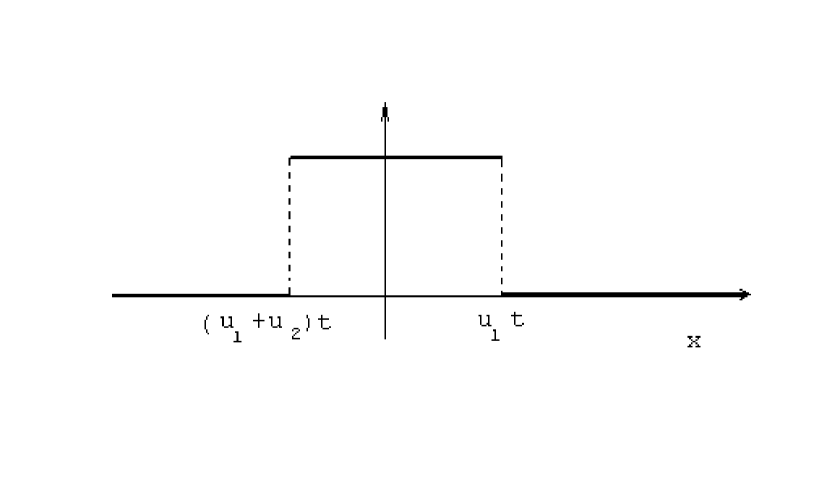
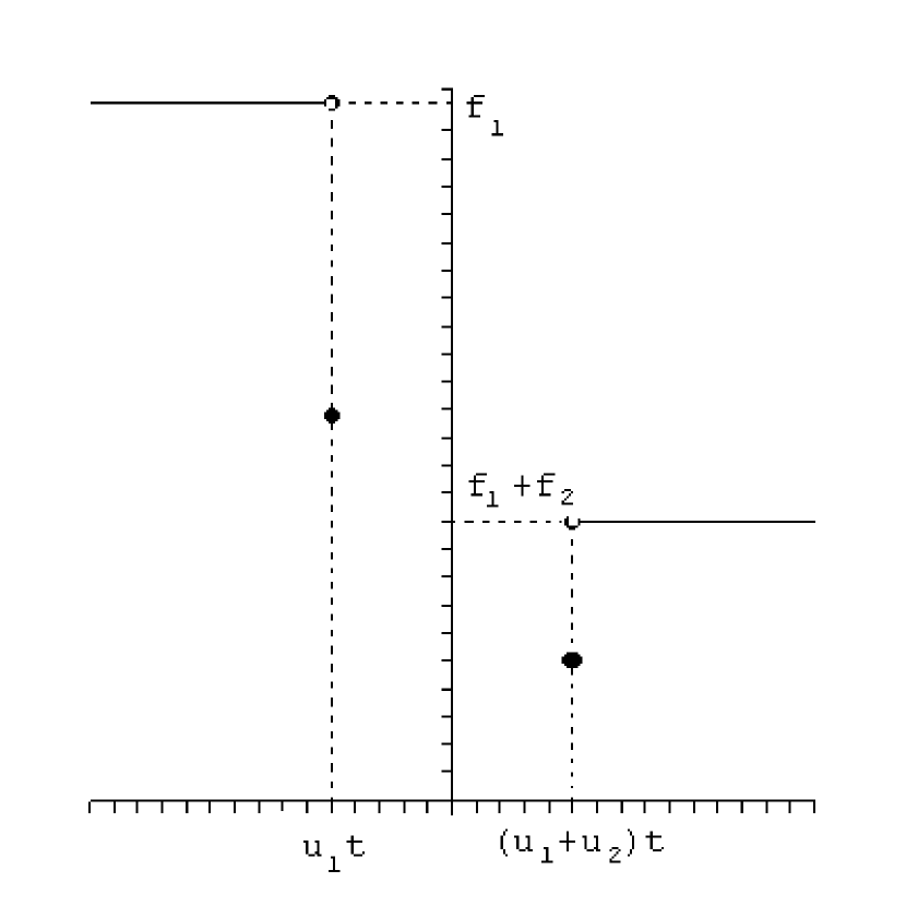
fFP(t,x)={f1,x<u1t,f12,x=u1t,0,u1t<x<(u1+u2)t,f1+f22,x=(u1+u2)t,f1+f2,x>(u1+u2)t.subscript𝑓𝐹𝑃𝑡𝑥casessubscript𝑓1x<u1t,subscript𝑓12x=u1t,0u1t<x<(u1+u2)t,subscript𝑓1subscript𝑓22x=(u1+u2)t,subscript𝑓1subscript𝑓2x>(u1+u2)t.f_{FP}(t,x)=\begin{cases}f_{1},&\text{$x<u_{1}t$,}\\ \dfrac{f_{1}}{2},&\text{$x=u_{1}t$,}\\ 0,&\text{$u_{1}t<x<(u_{1}+u_{2})t$,}\\ \dfrac{f_{1}+f_{2}}{2},&\text{$x=(u_{1}+u_{2})t$,}\\ f_{1}+f_{2},&\text{$x>(u_{1}+u_{2})t$.}\\ \end{cases}

Further, from (36) we find the solution of the gas dynamic system with smooth initial data uε(t,x)=limσ0u^ε(t,x)superscript𝑢𝜀𝑡𝑥subscript𝜎0subscript^𝑢𝜀𝑡𝑥u^{\varepsilon}(t,x)=\lim\limits_{\sigma\rightarrow 0}\hat{u}_{\varepsilon}(t,x) as follows:

uε(t,x)={u1,x<x^1ε,u1+Nε(t,x)Fε(t,x),x^1εxx^2ε,u1+u2,x>x^2ε.superscript𝑢𝜀𝑡𝑥casessubscript𝑢1x<x^1ε,subscript𝑢1superscript𝑁𝜀𝑡𝑥superscript𝐹𝜀𝑡𝑥x^1εxx^2ε,subscript𝑢1subscript𝑢2x>x^2ε.u^{\varepsilon}(t,x)=\begin{cases}u_{1},&\text{$x<\hat{x}^{\varepsilon}_{1}$,}\\ u_{1}+\dfrac{N^{\varepsilon}(t,x)}{F^{\varepsilon}(t,x)},&\text{$\hat{x}^{\varepsilon}_{1}\leq x\leq\hat{x}^{\varepsilon}_{2}$,}\\ u_{1}+u_{2},&\text{$x>\hat{x}^{\varepsilon}_{2}$.}\\ \end{cases}

It can be shown that

limε0Nε(t,x)Fε(t,x)=limε0u2u2t+2ε(x(u1+u22)t)+u22=xtu1.subscript𝜀0superscript𝑁𝜀𝑡𝑥superscript𝐹𝜀𝑡𝑥subscript𝜀0subscript𝑢2subscript𝑢2𝑡2𝜀𝑥subscript𝑢1subscript𝑢22𝑡subscript𝑢22𝑥𝑡subscript𝑢1\lim\limits_{\varepsilon\rightarrow 0}\dfrac{N^{\varepsilon}(t,x)}{F^{\varepsilon}(t,x)}=\lim\limits_{\varepsilon\rightarrow 0}\dfrac{u_{2}}{u_{2}t+2\varepsilon}(x-(u_{1}+\dfrac{u_{2}}{2})t)+\dfrac{u_{2}}{2}=\dfrac{x}{t}-u_{1}.

Thus, we get the following solution for u(t,x)=limε0uε(t,x)𝑢𝑡𝑥subscript𝜀0superscript𝑢𝜀𝑡𝑥u(t,x)=\lim\limits_{\varepsilon\rightarrow 0}u^{\varepsilon}(t,x):

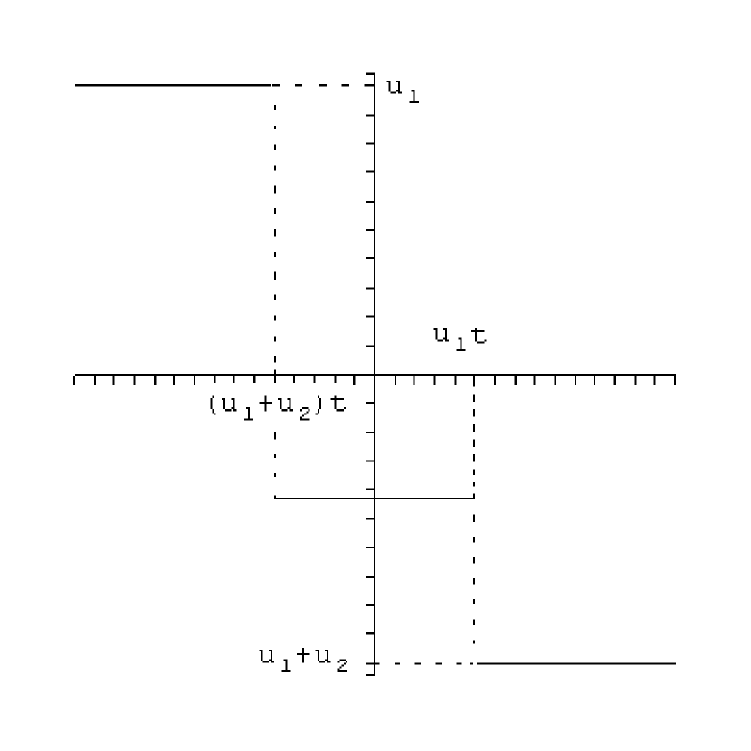
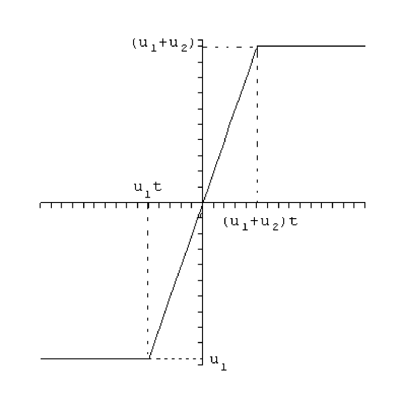
uFP(t,x)={u1,x<u1t,xt,u1tx(u1+u2)t,u1+u2,x>(u1+u2)t.subscript𝑢𝐹𝑃𝑡𝑥casessubscript𝑢1x<u1t,𝑥𝑡u1tx(u1+u2)t,subscript𝑢1subscript𝑢2x>(u1+u2)t.u_{FP}(t,x)=\begin{cases}u_{1},&\text{$x<u_{1}t$,}\\ \dfrac{x}{t},&\text{$u_{1}t\leq x\leq(u_{1}+u_{2})t$,}\\ u_{1}+u_{2},&\text{$x>(u_{1}+u_{2})t$.}\\ \end{cases}

We can see that the velocity includes the rarefaction wave (see Fig.1). This is a well known self-similar solution to the Riemann problem with constant left-hand and right-hand states for the Burgers equation ([29]).
Refer to caption

Refer to caption

Figure 1. Density and velocity, u2>0.subscript𝑢20u_{2}>0.

It is interesting to note that if we first compute the limit in ε𝜀\varepsilon we get the solution u(t,x)=u1+u2θ(x(u1+u22)t)𝑢𝑡𝑥subscript𝑢1subscript𝑢2𝜃𝑥subscript𝑢1subscript𝑢22𝑡u(t,x)=u_{1}+u_{2}\theta(x-(u_{1}+\dfrac{u_{2}}{2})t), which is unstable with respect to small perturbations.

2. u2<0subscript𝑢20u_{2}<0 (the velocity of x^2εsubscriptsuperscript^𝑥𝜀2\hat{x}^{\varepsilon}_{2} is higher than the velocity of x^1εsubscriptsuperscript^𝑥𝜀1\hat{x}^{\varepsilon}_{1}). From (34) and (36) we find as before (see Fig.2)
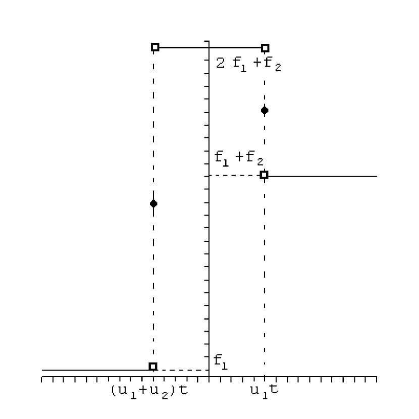
fFP(t,x)={f1,x<(u1+u2)t,3f1+f22,x=(u1+u2)t,2f1+f2,(u1+u2)t<x<u1t,3f1+2f22,x=u1t,f1+f2,x>u1t,subscript𝑓𝐹𝑃𝑡𝑥casessubscript𝑓1x<(u1+u2)t,3subscript𝑓1subscript𝑓22x=(u1+u2)t,2subscript𝑓1subscript𝑓2(u1+u2)t<x<u1t,3subscript𝑓12subscript𝑓22x=u1t,subscript𝑓1subscript𝑓2x>u1t,f_{FP}(t,x)=\begin{cases}f_{1},&\text{$x<(u_{1}+u_{2})t$,}\\ \dfrac{3f_{1}+f_{2}}{2},&\text{$x=(u_{1}+u_{2})t$,}\\ 2f_{1}+f_{2},&\text{$(u_{1}+u_{2})t<x<u_{1}t$,}\\ \dfrac{3f_{1}+2f_{2}}{2},&\text{$x=u_{1}t$,}\\ f_{1}+f_{2},&\text{$x>u_{1}t$,}\\ \end{cases}
uFP(t,x)={u1,x<(u1+u2)t,u1+f1+f22f1+f2u2,(u1+u2)txu1t,u1+u2,x>u1t.subscript𝑢𝐹𝑃𝑡𝑥casessubscript𝑢1x<(u1+u2)t,subscript𝑢1subscript𝑓1subscript𝑓22subscript𝑓1subscript𝑓2subscript𝑢2(u1+u2)txu1t,subscript𝑢1subscript𝑢2x>u1t.u_{FP}(t,x)=\begin{cases}u_{1},&\text{$x<(u_{1}+u_{2})t$,}\\ u_{1}+\dfrac{f_{1}+f_{2}}{2f_{1}+f_{2}}u_{2},&\text{$(u_{1}+u_{2})t\leq x\leq u_{1}t$,}\\ u_{1}+u_{2},&\text{$x>u_{1}t$.}\\ \end{cases}

Refer to caption

Refer to caption

Figure 2. Density and velocity, u2<0.subscript𝑢20u_{2}<0.

5. The singular Riemann problem in the FP sense

By the singular Riemann problem we mean the Cauchy problem with the following data:

f0(x)=f1+f2θ(xx0)+f3δ(xx0)=freg0+fsing0,subscript𝑓0𝑥subscript𝑓1subscript𝑓2𝜃𝑥subscript𝑥0subscript𝑓3𝛿𝑥subscript𝑥0superscriptsubscript𝑓𝑟𝑒𝑔0superscriptsubscript𝑓𝑠𝑖𝑛𝑔0f_{0}(x)=f_{1}+f_{2}\theta(x-x_{0})+f_{3}\delta(x-x_{0})=f_{reg}^{0}+f_{sing}^{0}, (37)
u0(x)=u1+u2θ(xx0),subscript𝑢0𝑥subscript𝑢1subscript𝑢2𝜃𝑥subscript𝑥0u_{0}(x)=u_{1}+u_{2}\theta(x-x_{0}), (38)

which differs from the classical Riemann problem (25), (26) by a singular part fsing0,superscriptsubscript𝑓𝑠𝑖𝑛𝑔0f_{sing}^{0}, the δ𝛿\delta - function of constant amplitude f3subscript𝑓3f_{3} concentrated at the jump of the density. We again set x0subscript𝑥0x_{0} equal to zero (without loss of generality).

Thus, we should adapt the definition of the generalized solution to the case of a singular density. As before we want to approximate initial data by smooth functions, the δ𝛿\delta-function will be instead naturally approximated in the space 𝒟()superscript𝒟\mathcal{D}^{\prime}(\mathbb{R}) of distributions.

Definition 3.

We call the couple of functions (fFP(t,x),uFP(t,x))subscript𝑓𝐹𝑃𝑡𝑥subscript𝑢𝐹𝑃𝑡𝑥(f_{FP}(t,x),u_{FP}(t,x)) a generalized solution to the problem (1) , (2), (37), (38) in the sense of free particles (FP), if

fFP(t,x)=limε0(limσ0ρσ,regε(t,x))+limε0(limσ0ρσ,singε(t,x))=freg(t,x)+fsing(t,x),subscript𝑓𝐹𝑃𝑡𝑥subscript𝜀0subscript𝜎0superscriptsubscript𝜌𝜎𝑟𝑒𝑔𝜀𝑡𝑥subscript𝜀0subscript𝜎0superscriptsubscript𝜌𝜎𝑠𝑖𝑛𝑔𝜀𝑡𝑥subscript𝑓𝑟𝑒𝑔𝑡𝑥subscript𝑓𝑠𝑖𝑛𝑔𝑡𝑥f_{FP}(t,x)=\lim\limits_{\varepsilon\rightarrow 0}(\lim\limits_{\sigma\rightarrow 0}\rho_{\sigma,reg}^{\varepsilon}(t,x))\,+\,\lim\limits_{\varepsilon\rightarrow 0}(\lim\limits_{\sigma\rightarrow 0}\rho_{\sigma,sing}^{\varepsilon}(t,x))\,=\,f_{reg}(t,x)\,+\,f_{sing}(t,x),
uFP(t,x)=limε0(limσ0u^σε(t,x)),subscript𝑢𝐹𝑃𝑡𝑥subscript𝜀0subscript𝜎0superscriptsubscript^𝑢𝜎𝜀𝑡𝑥u_{FP}(t,x)=\lim\limits_{\varepsilon\rightarrow 0}(\lim\limits_{\sigma\rightarrow 0}\hat{u}_{\sigma}^{\varepsilon}(t,x)),

where the limits are meant as pointwise at almost all points except for the singular part

limε0(limσ0ρσ,singε(t,x)),subscript𝜀0subscript𝜎0superscriptsubscript𝜌𝜎𝑠𝑖𝑛𝑔𝜀𝑡𝑥\lim\limits_{\varepsilon\rightarrow 0}(\lim\limits_{\sigma\rightarrow 0}\rho_{\sigma,sing}^{\varepsilon}(t,x)),

where the outer limit in ε𝜀\varepsilon is meant in the sense of distributions.

Here (ρσ,regε(t,x)+ρσ,singε(t,x),u^ε(t,x))superscriptsubscript𝜌𝜎𝑟𝑒𝑔𝜀𝑡𝑥superscriptsubscript𝜌𝜎𝑠𝑖𝑛𝑔𝜀𝑡𝑥superscript^𝑢𝜀𝑡𝑥(\rho_{\sigma,reg}^{\varepsilon}(t,x)\,+\,\rho_{\sigma,sing}^{\varepsilon}(t,x),\hat{u}^{\varepsilon}(t,x)) satisfy the system (23), (24) with initial data (f0,regε(x)+f0,singε(x),u0ε(x))superscriptsubscript𝑓0𝑟𝑒𝑔𝜀𝑥superscriptsubscript𝑓0𝑠𝑖𝑛𝑔𝜀𝑥superscriptsubscript𝑢0𝜀𝑥(f_{0,reg}^{\varepsilon}(x)\,+\,f_{0,sing}^{\varepsilon}(x),u_{0}^{\varepsilon}(x)) from the class C1(n)superscript𝐶1superscript𝑛C^{1}(\mathbb{R}^{n}) such that

limε0f0,regε(x)=f0reg(x),limε0u0ε(x)=u0(x)formulae-sequencesubscript𝜀0superscriptsubscript𝑓0𝑟𝑒𝑔𝜀𝑥superscriptsubscript𝑓0𝑟𝑒𝑔𝑥subscript𝜀0superscriptsubscript𝑢0𝜀𝑥subscript𝑢0𝑥\lim\limits_{\varepsilon\rightarrow 0}f_{0,reg}^{\varepsilon}(x)=f_{0}^{reg}(x),\quad\lim\limits_{\varepsilon\rightarrow 0}u_{0}^{\varepsilon}(x)=u_{0}(x)

for almost all fixed xn𝑥superscript𝑛x\in\mathbb{R}^{n} and

limε0f0,singε(x)=f0sing(x),subscript𝜀0superscriptsubscript𝑓0𝑠𝑖𝑛𝑔𝜀𝑥superscriptsubscript𝑓0𝑠𝑖𝑛𝑔𝑥\lim\limits_{\varepsilon\rightarrow 0}f_{0,sing}^{\varepsilon}(x)=f_{0}^{sing}(x),

the limit in ε𝜀\varepsilon being in the sense of distributions.


We are going to solve the singular Riemann problem with constant left and right states. To approximate the δ𝛿\delta-function we use the well known fact that

12πεex22εδ(x),ε0in𝒟().formulae-sequence12𝜋𝜀superscript𝑒superscript𝑥22𝜀𝛿𝑥𝜀0insuperscript𝒟\dfrac{1}{\sqrt{2\pi\varepsilon}}\,\,e^{-\frac{x^{2}}{2\varepsilon}}\rightarrow\delta(x),\quad\varepsilon\rightarrow 0\quad\text{in}\,\,\mathcal{D}^{\prime}(\mathbb{R}).

The part of the solution that relates to the regular part of the density (f3=0subscript𝑓30f_{3}=0) is found in Sec.4. Now we have to calculate the singular part of the density ρσ,singε(t,x)subscriptsuperscript𝜌𝜀𝜎𝑠𝑖𝑛𝑔𝑡𝑥\rho^{\varepsilon}_{\sigma,sing}(t,x) for f0,singε(x)=f312πεex22εsuperscriptsubscript𝑓0𝑠𝑖𝑛𝑔𝜀𝑥subscript𝑓312𝜋𝜀superscript𝑒superscript𝑥22𝜀f_{0,sing}^{\varepsilon}(x)=\,f_{3}\,\dfrac{1}{\sqrt{2\pi\varepsilon}}e^{-\frac{x^{2}}{2\varepsilon}}. As before we omit the index σ.𝜎\sigma.

From (18) we obtain:

ρsingε(t,x)=f32π(σ2t+ε)(exp[(u1tx)22(σ2t+ε)]Φ(D1σ,εσt)+\rho^{\varepsilon}_{sing}(t,x)=\dfrac{f_{3}}{\sqrt{2\pi(\sigma^{2}t+\varepsilon)}}\left(\exp\left[-\dfrac{(u_{1}t-x)^{2}}{2(\sigma^{2}t+\varepsilon)}\right]\Phi\left(\dfrac{D_{1}^{\sigma,\varepsilon}}{\sigma\sqrt{t}}\right)+\right.
+exp[((u1+u2)tx)22(σ2t+ε)]Φ(D2σ,εσt))+J2ε,σ=\left.+\exp\left[-\dfrac{((u_{1}+u_{2})t-x)^{2}}{2(\sigma^{2}t+\varepsilon)}\right]\Phi\left(-\dfrac{D_{2}^{\sigma,\varepsilon}}{\sigma\sqrt{t}}\right)\right)+J_{2}^{\varepsilon,\sigma}= (39)
=f32π(σ2t+ε)(G1σ,ε(t,x)Φ(D1σ,εσt)+G2σ,ε(t,x)Φ(D2σ,εσt))+J2ε,σ,absentsubscript𝑓32𝜋superscript𝜎2𝑡𝜀superscriptsubscript𝐺1𝜎𝜀𝑡𝑥Φsuperscriptsubscript𝐷1𝜎𝜀𝜎𝑡superscriptsubscript𝐺2𝜎𝜀𝑡𝑥Φsuperscriptsubscript𝐷2𝜎𝜀𝜎𝑡superscriptsubscript𝐽2𝜀𝜎=\dfrac{f_{3}}{\sqrt{2\pi(\sigma^{2}t+\varepsilon)}}\left(G_{1}^{\sigma,\varepsilon}(t,x)\Phi\left(\dfrac{D_{1}^{\sigma,\varepsilon}}{\sigma\sqrt{t}}\right)+G_{2}^{\sigma,\varepsilon}(t,x)\Phi\left(-\dfrac{D_{2}^{\sigma,\varepsilon}}{\sigma\sqrt{t}}\right)\right)+J_{2}^{\varepsilon,\sigma},

where

D1σ,ε=(u1tx)εσ2t+εε(σ2t+ε),superscriptsubscript𝐷1𝜎𝜀subscript𝑢1𝑡𝑥𝜀superscript𝜎2𝑡𝜀𝜀superscript𝜎2𝑡𝜀D_{1}^{\sigma,\varepsilon}=\dfrac{(u_{1}t-x)\sqrt{\varepsilon}}{\sqrt{\sigma^{2}t+\varepsilon}}-\sqrt{\varepsilon(\sigma^{2}t+\varepsilon)},
D2σ,ε=((u1+u2)tx)εσ2t+ε+ε(σ2t+ε),superscriptsubscript𝐷2𝜎𝜀subscript𝑢1subscript𝑢2𝑡𝑥𝜀superscript𝜎2𝑡𝜀𝜀superscript𝜎2𝑡𝜀D_{2}^{\sigma,\varepsilon}=\dfrac{((u_{1}+u_{2})t-x)\sqrt{\varepsilon}}{\sqrt{\sigma^{2}t+\varepsilon}}+\sqrt{\varepsilon(\sigma^{2}t+\varepsilon)},

and J2ε,σ=εεexp[s22ε(sx+(u22εs+u1+u22)t)22σ2t]𝑑ssuperscriptsubscript𝐽2𝜀𝜎superscriptsubscript𝜀𝜀superscript𝑠22𝜀superscript𝑠𝑥subscript𝑢22𝜀𝑠subscript𝑢1subscript𝑢22𝑡22superscript𝜎2𝑡differential-d𝑠J_{2}^{\varepsilon,\sigma}=\int\limits_{-\varepsilon}^{\varepsilon}\exp\left[-\dfrac{s^{2}}{2\varepsilon}-\dfrac{(s-x+(\dfrac{u_{2}}{2\varepsilon}s+u_{1}+\dfrac{u_{2}}{2})t)^{2}}{2\sigma^{2}t}\right]ds.

It can be checked that

J2ε,σ=f32πAσ,εexp[((u1+u22)tx)22Aσ,ε](Φ(K+σ,εσt)Φ(Kσ,εσt)),superscriptsubscript𝐽2𝜀𝜎subscript𝑓32𝜋superscript𝐴𝜎𝜀superscriptsubscript𝑢1subscript𝑢22𝑡𝑥22superscript𝐴𝜎𝜀Φsuperscriptsubscript𝐾𝜎𝜀𝜎𝑡Φsuperscriptsubscript𝐾𝜎𝜀𝜎𝑡J_{2}^{\varepsilon,\sigma}=\dfrac{f_{3}}{\sqrt{2\pi}\sqrt{A^{\sigma,\varepsilon}}}\exp\left[-\dfrac{((u_{1}+\frac{u_{2}}{2})t-x)^{2}}{2A^{\sigma,\varepsilon}}\right]\left(\Phi\left(\dfrac{K_{+}^{\sigma,\varepsilon}}{\sigma\sqrt{t}}\right)-\Phi\left(\dfrac{K_{-}^{\sigma,\varepsilon}}{\sigma\sqrt{t}}\right)\right),

where

Aσ,ε=σ2t+ε(u2t2ε+1)2,superscript𝐴𝜎𝜀superscript𝜎2𝑡𝜀superscriptsubscript𝑢2𝑡2𝜀12A^{\sigma,\varepsilon}=\sigma^{2}t+\varepsilon(\frac{u_{2}t}{2\varepsilon}+1)^{2}, (40)
Bσ,ε=ε(u2t2ε+1)((u1+u22)tx)Aσ,ε,superscript𝐵𝜎𝜀𝜀subscript𝑢2𝑡2𝜀1subscript𝑢1subscript𝑢22𝑡𝑥superscript𝐴𝜎𝜀B^{\sigma,\varepsilon}=\dfrac{\varepsilon(\frac{u_{2}t}{2\varepsilon}+1)((u_{1}+\frac{u_{2}}{2})t-x)}{\sqrt{A^{\sigma,\varepsilon}}}, (41)
K±σ,ε=1ε(Aσ,ε(±ε)+Bσ,ε).superscriptsubscript𝐾plus-or-minus𝜎𝜀1𝜀superscript𝐴𝜎𝜀plus-or-minus𝜀superscript𝐵𝜎𝜀K_{\pm}^{\sigma,\varepsilon}=\dfrac{1}{\sqrt{\varepsilon}}\left(\sqrt{A^{\sigma,\varepsilon}}(\pm\varepsilon)+B^{\sigma,\varepsilon}\right). (42)

It is easy to see that

D1ε=limσ0D1σ,ε=u1txε,D2ε=limσ0D2σ,ε=(u1+u2)txε,formulae-sequencesuperscriptsubscript𝐷1𝜀subscript𝜎0superscriptsubscript𝐷1𝜎𝜀subscript𝑢1𝑡𝑥𝜀superscriptsubscript𝐷2𝜀subscript𝜎0superscriptsubscript𝐷2𝜎𝜀subscript𝑢1subscript𝑢2𝑡𝑥𝜀D_{1}^{\varepsilon}=\lim\limits_{\sigma\rightarrow 0}D_{1}^{\sigma,\varepsilon}=u_{1}t-x-\varepsilon,\quad D_{2}^{\varepsilon}=\lim\limits_{\sigma\rightarrow 0}D_{2}^{\sigma,\varepsilon}=(u_{1}+u_{2})t-x-\varepsilon,
K±ε=limσ0K±σ,ε(ε)=(u2t2ε+1)(±ε)+(u1+u22)tx,superscriptsubscript𝐾plus-or-minus𝜀subscript𝜎0superscriptsubscript𝐾plus-or-minus𝜎𝜀𝜀subscript𝑢2𝑡2𝜀1plus-or-minus𝜀subscript𝑢1subscript𝑢22𝑡𝑥K_{\pm}^{\varepsilon}=\lim\limits_{\sigma\rightarrow 0}K_{\pm}^{\sigma,\varepsilon}(\varepsilon)=(\dfrac{u_{2}t}{2\varepsilon}+1)(\pm\varepsilon)+(u_{1}+\dfrac{u_{2}}{2})t-x,

i.e. Kε=D1ε=Cεsuperscriptsubscript𝐾𝜀superscriptsubscript𝐷1𝜀superscriptsubscript𝐶𝜀K_{-}^{\varepsilon}=D_{1}^{\varepsilon}=C_{-}^{\varepsilon}, K+ε=D2ε=C+εsuperscriptsubscript𝐾𝜀superscriptsubscript𝐷2𝜀superscriptsubscript𝐶𝜀K_{+}^{\varepsilon}=D_{2}^{\varepsilon}=C_{+}^{\varepsilon}. Therefore, in this case we also have two jump points x^1ε=u1tεsuperscriptsubscript^𝑥1𝜀subscript𝑢1𝑡𝜀\hat{x}_{1}^{\varepsilon}=u_{1}t-\varepsilon and x^2ε=(u1+u2)t+εsuperscriptsubscript^𝑥2𝜀subscript𝑢1subscript𝑢2𝑡𝜀\hat{x}_{2}^{\varepsilon}=(u_{1}+u_{2})t+\varepsilon.

We have to consider two cases u2>0subscript𝑢20u_{2}>0 and u2<0,subscript𝑢20u_{2}<0, as before. But for f0sing(x)=superscriptsubscript𝑓0𝑠𝑖𝑛𝑔𝑥absentf_{0}^{sing}(x)= =f3δ(x)absentsubscript𝑓3𝛿𝑥=f_{3}\,\delta(x) we obtain the same result:

fsing(t,x)=limε0limσ0ρsingε(t,x)=12f3(δ(xu1t)+δ(x(u1+u2)t)).subscript𝑓𝑠𝑖𝑛𝑔𝑡𝑥subscript𝜀0subscript𝜎0subscriptsuperscript𝜌𝜀𝑠𝑖𝑛𝑔𝑡𝑥12subscript𝑓3𝛿𝑥subscript𝑢1𝑡𝛿𝑥subscript𝑢1subscript𝑢2𝑡f_{sing}(t,x)=\lim\limits_{\varepsilon\rightarrow 0}\lim\limits_{\sigma\rightarrow 0}\rho^{\varepsilon}_{sing}(t,x)=\dfrac{1}{2}f_{3}(\delta(x-u_{1}t)+\delta(x-(u_{1}+u_{2})t)).

Thus, we have two δ𝛿\delta-functions with equal amplitudes 12F(t)12𝐹𝑡\dfrac{1}{2}F(t), which move with the jump points.

Further, we can find the regular part of the density freg(t,x)=limε0limσ0ρregε(t,x)subscript𝑓𝑟𝑒𝑔𝑡𝑥subscript𝜀0subscript𝜎0superscriptsubscript𝜌𝑟𝑒𝑔𝜀𝑡𝑥f_{reg}(t,x)=\lim\limits_{\varepsilon\rightarrow 0}\lim\limits_{\sigma\rightarrow 0}\rho_{reg}^{\varepsilon}(t,x), where

ρregε(t,x)=f1Φ(Cεσt)+(f1+f2)Φ(C+εσt)+I1.superscriptsubscript𝜌𝑟𝑒𝑔𝜀𝑡𝑥subscript𝑓1Φsuperscriptsubscript𝐶𝜀𝜎𝑡subscript𝑓1subscript𝑓2Φsuperscriptsubscript𝐶𝜀𝜎𝑡subscript𝐼1\rho_{reg}^{\varepsilon}(t,x)=f_{1}\Phi\left(\dfrac{C_{-}^{\varepsilon}}{\sigma\sqrt{t}}\right)+(f_{1}+f_{2})\Phi\left(-\dfrac{C_{+}^{\varepsilon}}{\sigma\sqrt{t}}\right)+I_{1}. (43)

Analogously, from (13) we can calculate the velocity u^(t,x)^𝑢𝑡𝑥\hat{u}(t,x):

u^ε(t,x)=u1+u2(f1+f2)Φ(C+εσt)+I2ε,σ+f3u22π(σ2t+ε)G2σ,ε(t,x)Φ(D2σ,εσt)+J3ε,σρε(t,x),superscript^𝑢𝜀𝑡𝑥subscript𝑢1subscript𝑢2subscript𝑓1subscript𝑓2Φsuperscriptsubscript𝐶𝜀𝜎𝑡superscriptsubscript𝐼2𝜀𝜎subscript𝑓3subscript𝑢22𝜋superscript𝜎2𝑡𝜀superscriptsubscript𝐺2𝜎𝜀𝑡𝑥Φsuperscriptsubscript𝐷2𝜎𝜀𝜎𝑡superscriptsubscript𝐽3𝜀𝜎superscript𝜌𝜀𝑡𝑥\hat{u}^{\varepsilon}(t,x)=u_{1}+\dfrac{u_{2}(f_{1}+f_{2})\Phi\left(-\frac{C_{+}^{\varepsilon}}{\sigma\sqrt{t}}\right)+I_{2}^{\varepsilon,\sigma}+\dfrac{f_{3}u_{2}}{\sqrt{2\pi(\sigma^{2}t+\varepsilon)}}G_{2}^{\sigma,\varepsilon}(t,x)\Phi\left(-\frac{D_{2}^{\sigma,\varepsilon}}{\sigma\sqrt{t}}\right)+J_{3}^{\varepsilon,\sigma}}{\rho^{\varepsilon}(t,x)},

where

J3ε,σ=f32πGσ,ε(t,x)(u2tε2εAσ,εσ[e(K+σ,ε)22tσ2e(Kσ,ε)22tσ2]+J_{3}^{\varepsilon,\sigma}=\dfrac{f_{3}}{\sqrt{2\pi}}G^{\sigma,\varepsilon}(t,x)\left(\dfrac{u_{2}\sqrt{t\varepsilon}}{2\varepsilon A^{\sigma,\varepsilon}}\sigma\left[e^{-\frac{(K^{\sigma,\varepsilon}_{+})^{2}}{2t\sigma^{2}}}-e^{-\frac{(K^{\sigma,\varepsilon}_{-})^{2}}{2t\sigma^{2}}}\right]+\right.
+1Aσ,ε(u22u2Bσ,ε2εAσ,ε)[Φ(K+σ,εσt)Φ(Kσ,εσt)]),\left.+\dfrac{1}{\sqrt{A^{\sigma,\varepsilon}}}\left(\dfrac{u_{2}}{2}-\dfrac{u_{2}B^{\sigma,\varepsilon}}{2\varepsilon A^{\sigma,\varepsilon}}\right)\left[\Phi\left(\dfrac{K_{+}^{\sigma,\varepsilon}}{\sigma\sqrt{t}}\right)-\Phi\left(\dfrac{K_{-}^{\sigma,\varepsilon}}{\sigma\sqrt{t}}\right)\right]\right),
Gσ,ε(t,x)=exp[((u1+u22)tx)22Aσ,ε],superscript𝐺𝜎𝜀𝑡𝑥superscriptsubscript𝑢1subscript𝑢22𝑡𝑥22superscript𝐴𝜎𝜀G^{\sigma,\varepsilon}(t,x)=\exp\left[-\dfrac{((u_{1}+\frac{u_{2}}{2})t-x)^{2}}{2A^{\sigma,\varepsilon}}\right],
G2σ,ε(t,x)=exp[((u1+u2)tx)22(σ2t+ε)].superscriptsubscript𝐺2𝜎𝜀𝑡𝑥superscriptsubscript𝑢1subscript𝑢2𝑡𝑥22superscript𝜎2𝑡𝜀G_{2}^{\sigma,\varepsilon}(t,x)=\exp\left[-\dfrac{((u_{1}+u_{2})t-x)^{2}}{2(\sigma^{2}t+\varepsilon)}\right].

The expressions for ρε(t,x)=ρregε(t,x)+ρsingε(t,x)superscript𝜌𝜀𝑡𝑥superscriptsubscript𝜌𝑟𝑒𝑔𝜀𝑡𝑥superscriptsubscript𝜌𝑠𝑖𝑛𝑔𝜀𝑡𝑥\rho^{\varepsilon}(t,x)\,=\,\rho_{reg}^{\varepsilon}(t,x)\,+\,\rho_{sing}^{\varepsilon}(t,x) and I2ε,σsuperscriptsubscript𝐼2𝜀𝜎I_{2}^{\varepsilon,\sigma} have been given in (43), (39) and (35), respectively.

1. u2>0subscript𝑢20u_{2}>0 then:

uε(t,x)={u1,x<x^1ε,u1+f32πTεGε(t,x)+Nεf32πε2ε2ε+u2tGε(t,x)+Fε,x^1εxx^2ε,u1+u2,x>x^2ε,superscript𝑢𝜀𝑡𝑥casessubscript𝑢1x<x^1ε,subscript𝑢1subscript𝑓32𝜋superscript𝑇𝜀superscript𝐺𝜀𝑡𝑥superscript𝑁𝜀subscript𝑓32𝜋𝜀2𝜀2𝜀subscript𝑢2𝑡superscript𝐺𝜀𝑡𝑥superscript𝐹𝜀x^1εxx^2ε,subscript𝑢1subscript𝑢2x>x^2ε,u^{\varepsilon}(t,x)=\begin{cases}u_{1},&\text{$x<\hat{x}^{\varepsilon}_{1}$,}\\ u_{1}+\dfrac{\dfrac{f_{3}}{\sqrt{2\pi}}T^{\varepsilon}G^{\varepsilon}(t,x)+N^{\varepsilon}}{\dfrac{f_{3}}{\sqrt{2\pi\varepsilon}}\dfrac{2\varepsilon}{2\varepsilon+u_{2}t}G^{\varepsilon}(t,x)+F^{\varepsilon}},&\text{$\hat{x}^{\varepsilon}_{1}\leq x\leq\hat{x}^{\varepsilon}_{2}$,}\\ u_{1}+u_{2},&\text{$x>\hat{x}^{\varepsilon}_{2}$,}\\ \end{cases}

where

Tε=limσ01Aσ,ε(u22u2Bσ,ε2εAσ,ε)=u222ε((u1+u22)tx)u2(2ε+u2t)2ε,superscript𝑇𝜀subscript𝜎01superscript𝐴𝜎𝜀subscript𝑢22subscript𝑢2superscript𝐵𝜎𝜀2𝜀superscript𝐴𝜎𝜀subscript𝑢222𝜀subscript𝑢1subscript𝑢22𝑡𝑥subscript𝑢2superscript2𝜀subscript𝑢2𝑡2𝜀T^{\varepsilon}=\lim\limits_{\sigma\rightarrow 0}\dfrac{1}{\sqrt{A^{\sigma,\varepsilon}}}\left(\dfrac{u_{2}}{2}-\dfrac{u_{2}B^{\sigma,\varepsilon}}{2\varepsilon A^{\sigma,\varepsilon}}\right)=\dfrac{u_{2}}{2}-\dfrac{2\varepsilon((u_{1}+\dfrac{u_{2}}{2})t-x)u_{2}}{(2\varepsilon+u_{2}t)^{2}\sqrt{\varepsilon}},

Therefore

uFP(t,x)=limε0uε(t,x)={u1,x<u1t,xt,u1tx(u1+u2)t,u1+u2,x>x^(u1+u2)t.subscript𝑢𝐹𝑃𝑡𝑥subscript𝜀0superscript𝑢𝜀𝑡𝑥casessubscript𝑢1x<u1t,𝑥𝑡u1tx(u1+u2)t,subscript𝑢1subscript𝑢2x>x^(u1+u2)t.u_{FP}(t,x)=\lim\limits_{\varepsilon\rightarrow 0}u^{\varepsilon}(t,x)=\begin{cases}u_{1},&\text{$x<u_{1}t$,}\\ \dfrac{x}{t},&\text{$u_{1}t\leq x\leq(u_{1}+u_{2})t$,}\\ u_{1}+u_{2},&\text{$x>\hat{x}^{(}u_{1}+u_{2})t$.}\\ \end{cases}

Further, from (43), (39) we find the density as follows:

fFP(t,x)=12f3(δ(xu1t)+δ(x(u1+u2)t))+{f1,x<u1t,f12,x=u1t,0,u1t<x<(u1+u2)t,f1+f22,x=(u1+u2)t,f1+f2,x>(u1+u2)t,subscript𝑓𝐹𝑃𝑡𝑥12subscript𝑓3𝛿𝑥subscript𝑢1𝑡𝛿𝑥subscript𝑢1subscript𝑢2𝑡casessubscript𝑓1x<u1t,subscript𝑓12x=u1t,0u1t<x<(u1+u2)t,subscript𝑓1subscript𝑓22x=(u1+u2)t,subscript𝑓1subscript𝑓2x>(u1+u2)t,f_{FP}(t,x)=\dfrac{1}{2}f_{3}(\delta(x-u_{1}t)+\delta(x-(u_{1}+u_{2})t))+\begin{cases}f_{1},&\text{$x<u_{1}t$,}\\ \dfrac{f_{1}}{2},&\text{$x=u_{1}t$,}\\ 0,&\text{$u_{1}t<x<(u_{1}+u_{2})t$,}\\ \dfrac{f_{1}+f_{2}}{2},&\text{$x=(u_{1}+u_{2})t$,}\\ f_{1}+f_{2},&\text{$x>(u_{1}+u_{2})t$,}\\ \end{cases}

2. If u2<0,subscript𝑢20u_{2}<0, we have

uε(t,x)={u1,x<x^1ε,u1+u2(f1+f2)Nε+f32πε(G2εεTεGε)2f1+f2+Fε+f32πε(G1ε+G2ε2ε2ε+u2tGε),x^1εxx^2ε,u1+u2,x>x^2ε,superscript𝑢𝜀𝑡𝑥casessubscript𝑢1x<x^1ε,subscript𝑢1subscript𝑢2subscript𝑓1subscript𝑓2superscript𝑁𝜀subscript𝑓32𝜋𝜀superscriptsubscript𝐺2𝜀𝜀superscript𝑇𝜀superscript𝐺𝜀2subscript𝑓1subscript𝑓2superscript𝐹𝜀subscript𝑓32𝜋𝜀superscriptsubscript𝐺1𝜀superscriptsubscript𝐺2𝜀2𝜀2𝜀subscript𝑢2𝑡superscript𝐺𝜀x^1εxx^2ε,subscript𝑢1subscript𝑢2x>x^2ε,u^{\varepsilon}(t,x)=\begin{cases}u_{1},&\text{$x<\hat{x}^{\varepsilon}_{1}$,}\\ u_{1}+\dfrac{u_{2}(f_{1}+f_{2})-N^{\varepsilon}+\dfrac{f_{3}}{\sqrt{2\pi\varepsilon}}(G_{2}^{\varepsilon}-\varepsilon T^{\varepsilon}G^{\varepsilon})}{2f_{1}+f_{2}+F^{\varepsilon}+\dfrac{f_{3}}{\sqrt{2\pi\varepsilon}}(G_{1}^{\varepsilon}+G_{2}^{\varepsilon}-\dfrac{2\varepsilon}{2\varepsilon+u_{2}t}G^{\varepsilon})},&\text{$\hat{x}^{\varepsilon}_{1}\leq x\leq\hat{x}^{\varepsilon}_{2}$,}\\ u_{1}+u_{2},&\text{$x>\hat{x}^{\varepsilon}_{2}$,}\\ \end{cases}

where G1εexp[(u1tx)22ε]superscriptsubscript𝐺1𝜀superscriptsubscript𝑢1𝑡𝑥22𝜀G_{1}^{\varepsilon}\equiv\exp\left[-\dfrac{(u_{1}t-x)^{2}}{2\varepsilon}\right], G2εexp[((u1+u2)tx)22ε]superscriptsubscript𝐺2𝜀superscriptsubscript𝑢1subscript𝑢2𝑡𝑥22𝜀G_{2}^{\varepsilon}\equiv\exp\left[-\dfrac{((u_{1}+u_{2})t-x)^{2}}{2\varepsilon}\right].

Thus,

uFP(t,x)={u1,x<(u1+u2)t,u1+(f1+f2)2f1+f2u2,(u1+u2)txu1t,u1+u2,x>u1t.subscript𝑢𝐹𝑃𝑡𝑥casessubscript𝑢1x<(u1+u2)t,subscript𝑢1subscript𝑓1subscript𝑓22subscript𝑓1subscript𝑓2subscript𝑢2(u1+u2)txu1t,subscript𝑢1subscript𝑢2x>u1t.u_{FP}(t,x)=\begin{cases}u_{1},&\text{$x<(u_{1}+u_{2})t$,}\\ u_{1}+\dfrac{(f_{1}+f_{2})}{2f_{1}+f_{2}}u_{2},&\text{$(u_{1}+u_{2})t\leq x\leq u_{1}t$,}\\ u_{1}+u_{2},&\text{$x>u_{1}t$.}\\ \end{cases}

As a consequence, for the velocity we obtain the same result as in the non-singular case. Analogously,

fFP(t,x)=12f3(δ(xu1t)+δ(x(u1+u2)t))+{f1,x<(u1+u2)t,3f1+f22,x=(u1+u2)t,2f1+f2,(u1+u2)t<x<u1t,3f1+2f22,x=u1t,f1+f2,x>u1t.subscript𝑓𝐹𝑃𝑡𝑥12subscript𝑓3𝛿𝑥subscript𝑢1𝑡𝛿𝑥subscript𝑢1subscript𝑢2𝑡casessubscript𝑓1x<(u1+u2)t,3subscript𝑓1subscript𝑓22x=(u1+u2)t,2subscript𝑓1subscript𝑓2(u1+u2)t<x<u1t,3subscript𝑓12subscript𝑓22x=u1t,subscript𝑓1subscript𝑓2x>u1t.f_{FP}(t,x)=\dfrac{1}{2}f_{3}(\delta(x-u_{1}t)+\delta(x-(u_{1}+u_{2})t))+\begin{cases}f_{1},&\text{$x<(u_{1}+u_{2})t$,}\\ \dfrac{3f_{1}+f_{2}}{2},&\text{$x=(u_{1}+u_{2})t$,}\\ 2f_{1}+f_{2},&\text{$(u_{1}+u_{2})t<x<u_{1}t$,}\\ \dfrac{3f_{1}+2f_{2}}{2},&\text{$x=u_{1}t$,}\\ f_{1}+f_{2},&\text{$x>u_{1}t$.}\\ \end{cases}

6. Singularity arising from smooth data

We are going to show that at the point of formation of a singularity from smooth initial data in the solution to the pressureless gas dynamics model a δ𝛿\delta – function appears in the density component. For the sake of simplicity we again restrict ourselves to the 1D case.

Theorem 1.

(Asymptotics of the approximating solution) Let the initial data (f0,u0)subscript𝑓0subscript𝑢0\,(f_{0},\,u_{0})\, for the system (1), (2) be at least Cmsuperscript𝐶𝑚C^{m} – smooth and bounded, m2.𝑚2m\geq 2. Assume that there exists an instant 0<t<,0subscript𝑡0<t_{*}<\infty, such that t=infx(1u0(x))subscript𝑡subscriptinfimum𝑥1subscriptsuperscript𝑢0𝑥t_{*}=\inf\limits_{x\in\mathbb{R}}\left(-\frac{1}{u^{\prime}_{0}(x)}\right) and u(k)(s)=0,k=1,,m1,formulae-sequencesuperscript𝑢𝑘subscript𝑠0𝑘1𝑚1u^{(k)}(s_{*})=0,\,k=1,...,m-1, however u(m)(s)superscript𝑢𝑚subscript𝑠u^{(m)}(s_{*}) does not vanish at the point s(t,x),subscript𝑠subscript𝑡subscript𝑥s_{*}(t_{*},x_{*}), where ssubscript𝑠s_{*} is a solution to the equation u0(s)t=xs.subscript𝑢0𝑠subscript𝑡subscript𝑥𝑠u_{0}(s)\,t_{*}\,=\,x_{*}-\,s. Here xsubscript𝑥\,x_{*} is such that the line y=xst𝑦subscript𝑥𝑠subscript𝑡y=\frac{x_{*}-s}{t_{*}} intersects the graph of the initial velocity y=u0(s)𝑦subscript𝑢0𝑠y=u_{0}(s) at a unique point and it is tangent to the graph.

Then at the moment t=t𝑡subscript𝑡t=t_{*} the following properties of the function ρσ(t,x),subscript𝜌𝜎𝑡𝑥\rho_{\sigma}(t,x), entering the solution (ρσ,u^σ)subscript𝜌𝜎subscript^𝑢𝜎(\rho_{\sigma},\hat{u}_{\sigma}) to the system (23), (24) hold:

  • ρσ(t,x)B(x,t)f0(s)σm1m,σ0,formulae-sequencesimilar-tosubscript𝜌𝜎subscript𝑡subscript𝑥𝐵subscript𝑥subscript𝑡subscript𝑓0subscript𝑠superscript𝜎𝑚1𝑚𝜎0\rho_{\sigma}(t_{*},x_{*})\,\sim\,B(x_{*},t_{*})\,f_{0}(s_{*})\,\sigma^{-\frac{m-1}{m}},\,\quad\sigma\to 0, (44)

    where

    B(x,t)=Km|u0(s)|m12m|u0(m)(s)|1m,Km=12m12mmπ(m!)1mΓ(12m),formulae-sequence𝐵subscript𝑥subscript𝑡subscript𝐾𝑚superscriptsuperscriptsubscript𝑢0subscript𝑠𝑚12𝑚superscriptsuperscriptsubscript𝑢0𝑚subscript𝑠1𝑚subscript𝐾𝑚1superscript2𝑚12𝑚𝑚𝜋superscript𝑚1𝑚Γ12𝑚B(x_{*},t_{*})\,=\,K_{m}\,\frac{|u_{0}^{\prime}(s_{*})|^{\frac{m-1}{2m}}}{|u_{0}^{(m)}(s_{*})|^{\frac{1}{m}}},\qquad K_{m}\,=\,\frac{1}{2^{\frac{m-1}{2m}}\,m\,\sqrt{\pi}}\,(m!)^{\frac{1}{m}}\,\Gamma\left(\frac{1}{2m}\right),

    similar-to\sim means that the quotient of the left-hand side by the right-hand side converges to 111 as σ0;𝜎0\sigma\to 0;

  • ρσ(t,x)f0(s0(t,x)),σ0,forxx,formulae-sequencesubscript𝜌𝜎subscript𝑡𝑥subscript𝑓0subscript𝑠0subscript𝑡𝑥formulae-sequence𝜎0for𝑥subscript𝑥\rho_{\sigma}(t_{*},x)\,\to\,f_{0}(s_{0}(t_{*},x)),\quad\sigma\to 0,\quad\mbox{for}\,x\neq x_{*}, (45)

    where the function s0(t,x)subscript𝑠0𝑡𝑥s_{0}(t,x) has been introduced in the proof of Proposition 1.

Proof.

Proceeding as in the proof of Proposition 1 we can readily obtain the property (45). Thus, let us dwell on the property (44).

Let us analyze the formula (18) at the point (t,x)subscript𝑡subscript𝑥(t_{*},x_{*}). To that end we note that since u0(s)t=xssubscript𝑢0subscript𝑠subscript𝑡subscript𝑥subscript𝑠\,u_{0}(s_{*})\,t_{*}=x_{*}-s_{*}\, and t=1u0(s),subscript𝑡1subscript𝑢0subscript𝑠\,t_{*}=-\frac{1}{u_{0}(s_{*})},\, for s𝑠\,s\, belonging to the ε𝜀\varepsilon - neighborhood Us(ε)subscript𝑈subscript𝑠𝜀U_{s_{*}}(\varepsilon) of the point ssubscript𝑠s_{*} we have

u0(s)t+sx=(u0(s)+u0(s)(ss)+1m!u0(m)(s)(ss)m)t+sx=u_{0}(s)\,t_{*}+s-x\,=\,(u_{0}(s_{*})+u^{\prime}_{0}(s_{*})\,(s-s_{*})+\frac{1}{m!}\,u^{(m)}_{0}(s_{**)}\,(s-s_{*})^{m})\,t_{*}\,+s-x=
=1m!u0(m)(s)(ss)mt(xx),=\frac{1}{m!}\,u^{(m)}_{0}(s_{**)}\,(s-s_{*})^{m}\,t_{*}-(x-x_{*}), (46)

with sUs(ε),subscript𝑠absentsubscript𝑈subscript𝑠𝜀s_{**}\in U_{s_{*}}(\varepsilon), ε>0.𝜀0\,\varepsilon>0.

Then from (18) we have

ρ(t,x)=12πtσf0(s)e(u0(s)t+sx)22σ2t𝑑s=𝜌subscript𝑡subscript𝑥12𝜋subscript𝑡𝜎subscriptsubscript𝑓0𝑠superscript𝑒superscriptsubscript𝑢0𝑠𝑡𝑠subscript𝑥22superscript𝜎2subscript𝑡differential-d𝑠absent\rho(t_{*},x_{*})\,=\,\dfrac{1}{\sqrt{2\pi t_{*}}\sigma}\,\int\limits_{\mathbb{R}}\,f_{0}(s)e^{-\frac{(u_{0}(s)t+s-x_{*})^{2}}{2\sigma^{2}t_{*}}}\,ds\,=
12πtσf0(s)e(u0(m)(s)tm!(ss)m)22σ2t𝑑s+limit-from12𝜋subscript𝑡𝜎subscriptsubscript𝑓0𝑠superscript𝑒superscriptsuperscriptsubscript𝑢0𝑚subscript𝑠subscript𝑡𝑚superscript𝑠subscript𝑠𝑚22superscript𝜎2subscript𝑡differential-d𝑠\dfrac{1}{\sqrt{2\pi t_{*}}\sigma}\,\int\limits_{\mathbb{R}}\,f_{0}(s)\,e^{-\frac{(\frac{u_{0}^{(m)}(s_{*})t_{*}}{m!}\,(s-s_{*})^{m})^{2}}{2\sigma^{2}t_{*}}}\,ds\,+
12πtσf0(s)(e(u0(s)t+sx)22σ2te(u0(m)(s)tm!(ss)m)22σ2t)𝑑s=12𝜋subscript𝑡𝜎subscriptsubscript𝑓0𝑠superscript𝑒superscriptsubscript𝑢0𝑠𝑡𝑠subscript𝑥22superscript𝜎2subscript𝑡superscript𝑒superscriptsuperscriptsubscript𝑢0𝑚subscript𝑠subscript𝑡𝑚superscript𝑠subscript𝑠𝑚22superscript𝜎2subscript𝑡differential-d𝑠absent\dfrac{1}{\sqrt{2\pi t_{*}}\sigma}\,\int\limits_{\mathbb{R}}\,f_{0}(s)\left(e^{-\frac{(u_{0}(s)t+s-x_{*})^{2}}{2\sigma^{2}t_{*}}}\,-\,e^{-\frac{(\frac{u_{0}^{(m)}(s_{*})t_{*}}{m!}\,(s-s_{*})^{m})^{2}}{2\sigma^{2}t_{*}}}\right)\,ds=
I1+I2.subscript𝐼1subscript𝐼2I_{1}+I_{2}.

The first integral I1subscript𝐼1I_{1} is equal to

σm1mIσ(t,x),superscript𝜎𝑚1𝑚subscript𝐼𝜎subscript𝑡subscript𝑥\sigma^{-\frac{m-1}{m}}\,I_{\sigma}(t_{*},x_{*}),

where Iσ(t,x)B(x,t)f0(s)subscript𝐼𝜎subscript𝑡subscript𝑥𝐵subscript𝑥subscript𝑡subscript𝑓0subscript𝑠I_{\sigma}(t_{*},x_{*})\to B(x_{*},t_{*})\,f_{0}(s_{*}) as σ0,𝜎0\sigma\to 0, where B(x,t)𝐵subscript𝑥subscript𝑡B(x_{*},t_{*}) is specified in the statement of Theorem 1. To evaluate Iσsubscript𝐼𝜎I_{\sigma} we have used the formula

ea2s2m𝑑s=Γ(12m)|a|1mm,a=const0.formulae-sequencesubscriptsuperscript𝑒superscript𝑎2superscript𝑠2𝑚differential-d𝑠Γ12𝑚superscript𝑎1𝑚𝑚𝑎const0\int\limits_{{\mathbb{R}}}\,e^{-a^{2}\,s^{2m}}\,ds\,=\,\frac{\Gamma\left(\frac{1}{2m}\right)}{|a|^{\frac{1}{m}}\,m},\quad a={\rm const}\neq 0.

Now let as prove that I20subscript𝐼20I_{2}\to 0 as σ0.𝜎0\sigma\to 0.

Let us choose ε>0𝜀0\varepsilon>0 so small that for all sUs(ε)𝑠subscript𝑈subscript𝑠𝜀s\in U_{s_{*}}(\varepsilon)

|e(u0(s)t+sx)22σ2te(u0(m)(s)tm!(ss)m)22σ2t|<σ.superscript𝑒superscriptsubscript𝑢0𝑠𝑡𝑠subscript𝑥22superscript𝜎2subscript𝑡superscript𝑒superscriptsuperscriptsubscript𝑢0𝑚subscript𝑠subscript𝑡𝑚superscript𝑠subscript𝑠𝑚22superscript𝜎2subscript𝑡𝜎\big{|}\,e^{-\frac{(u_{0}(s)t+s-x_{*})^{2}}{2\sigma^{2}t_{*}}}\,-\,e^{-\frac{(\frac{u_{0}^{(m)}(s_{*})t_{*}}{m!}\,(s-s_{*})^{m})^{2}}{2\sigma^{2}t_{*}}}\,\big{|}<\sigma.

Then

|I2|12πtσUs(ε)|f0(s)||e(u0(s)t+sx)22σ2te(u0(m)(s)tm!(ss)m)22σ2t|𝑑s+subscript𝐼2limit-from12𝜋subscript𝑡𝜎subscriptsubscript𝑈subscript𝑠𝜀subscript𝑓0𝑠superscript𝑒superscriptsubscript𝑢0𝑠𝑡𝑠subscript𝑥22superscript𝜎2subscript𝑡superscript𝑒superscriptsuperscriptsubscript𝑢0𝑚subscript𝑠subscript𝑡𝑚superscript𝑠subscript𝑠𝑚22superscript𝜎2subscript𝑡differential-d𝑠|I_{2}|\leq\dfrac{1}{\sqrt{2\pi t_{*}}\sigma}\,\int\limits_{U_{s_{*}}(\varepsilon)}\,|f_{0}(s)|\left|e^{-\frac{(u_{0}(s)t+s-x_{*})^{2}}{2\sigma^{2}t_{*}}}\,-\,e^{-\frac{(\frac{u_{0}^{(m)}(s_{*})t_{*}}{m!}\,(s-s_{*})^{m})^{2}}{2\sigma^{2}t_{*}}}\right|\,ds\,+
12πtσ\Us(ε)|f0(s)|(e(u0(s)t+sx)22σ2t+e(u0(m)(s)tm!(ss)m)22σ2t)𝑑s.12𝜋subscript𝑡𝜎subscript\subscript𝑈subscript𝑠𝜀subscript𝑓0𝑠superscript𝑒superscriptsubscript𝑢0𝑠𝑡𝑠subscript𝑥22superscript𝜎2subscript𝑡superscript𝑒superscriptsuperscriptsubscript𝑢0𝑚subscript𝑠subscript𝑡𝑚superscript𝑠subscript𝑠𝑚22superscript𝜎2subscript𝑡differential-d𝑠\dfrac{1}{\sqrt{2\pi t_{*}}\sigma}\,\int\limits_{{\mathbb{R}}\backslash U_{s_{*}}(\varepsilon)}\,|f_{0}(s)|\left(e^{-\frac{(u_{0}(s)t+s-x_{*})^{2}}{2\sigma^{2}t_{*}}}\,+\,e^{-\frac{(\frac{u_{0}^{(m)}(s_{*})t_{*}}{m!}\,(s-s_{*})^{m})^{2}}{2\sigma^{2}t_{*}}}\right)\,ds.

The first part in the right-hand side of the inequality due to the boundedness of f0subscript𝑓0f_{0} is less than constε,const𝜀\,{\rm const}\cdot\varepsilon,\, the second part tends to zero as σ0𝜎0\sigma\to 0 due to the boundness of f0.subscript𝑓0f_{0}. Since ε𝜀\varepsilon can be chosen arbitrarily small, the statement is proved. \square

Remark 6.

The following asymptotics of Kmsubscript𝐾𝑚K_{m} holds:

Km=2em,+O(lnm)m.formulae-sequencesubscript𝐾𝑚2𝑒𝑚𝑂𝑚𝑚K_{m}\,=\,\frac{\sqrt{2}}{e}\,m,+\,O(\ln m)\quad m\to\infty.
Theorem 2.

(Amplitude of the δlimit-from𝛿\delta- function) Let the initial data (f0,u0)subscript𝑓0subscript𝑢0\,(f_{0},\,u_{0})\, for the system (1), (2) be C1superscript𝐶1C^{1} – smooth and bounded and let the critical instant t=infx(1u0(x))subscript𝑡subscriptinfimum𝑥1subscriptsuperscript𝑢0𝑥t_{*}=\inf\limits_{x\in\mathbb{R}}\left(-\frac{1}{u^{\prime}_{0}(x)}\right) be positive and finite. Assume that the initial datum u0subscript𝑢0u_{0} is linear on the segment Ω=(x1,x2),Ωsubscript𝑥1subscript𝑥2\Omega=(x_{1},x_{2}), moreover, the second left-hand derivative u0′′(x10)superscriptsubscript𝑢0′′subscript𝑥10u_{0}^{\prime\prime}(x_{1}-0) at the point x1subscript𝑥1x_{1} and the second right-hand derivative u0′′(x2+0)superscriptsubscript𝑢0′′subscript𝑥20u_{0}^{\prime\prime}(x_{2}+0) at the point x2subscript𝑥2x_{2} do not vanish. Let xsubscript𝑥x_{*} be the unique point such that the line y=xst𝑦subscript𝑥𝑠subscript𝑡y=\frac{x_{*}-s}{t_{*}} and the graph of the initial velocity y=u0(s)𝑦subscript𝑢0𝑠y=u_{0}(s) have a common linear segment Ω¯=[s1,s2].¯Ωsubscript𝑠1subscript𝑠2\bar{\Omega}=[s_{1},s_{2}].

Then at the moment t=t𝑡subscript𝑡t=t_{*} at the point x=x𝑥subscript𝑥x=x_{*} the component of the density develops a δ𝛿\delta – singularity of amplitude

A(x)=s1s2f(s)𝑑s.𝐴subscript𝑥superscriptsubscriptsubscript𝑠1subscript𝑠2𝑓𝑠differential-d𝑠A(x_{*})\,=\int\limits_{s_{1}}^{s_{2}}\,f(s)\,ds. (47)
Proof.

We are going to prove that

ρσ(t,x)ϕ(x)𝑑xA(x)ϕ(x),σ0.formulae-sequencesubscriptsubscript𝜌𝜎subscript𝑡𝑥italic-ϕ𝑥differential-d𝑥𝐴subscript𝑥italic-ϕsubscript𝑥𝜎0\int\limits_{\mathbb{R}}\rho_{\sigma}(t_{*},x)\phi(x)\,dx\,\to\,A(x_{*})\phi(x_{*}),\qquad\sigma\to 0.

From (18) we have

ρ(t,x)ϕ(x)𝑑x=12πtσf0(s)e(u0(s)t+sx)22σ2tϕ(x)𝑑s𝑑x=subscript𝜌subscript𝑡𝑥italic-ϕ𝑥differential-d𝑥12𝜋subscript𝑡𝜎subscriptsubscriptsubscript𝑓0𝑠superscript𝑒superscriptsubscript𝑢0𝑠subscript𝑡𝑠𝑥22superscript𝜎2subscript𝑡italic-ϕ𝑥differential-d𝑠differential-d𝑥absent\int\limits_{\mathbb{R}}\rho(t_{*},x)\phi(x)\,dx\,=\,\dfrac{1}{\sqrt{2\pi t_{*}}\sigma}\,\int\limits_{\mathbb{R}}\,\int\limits_{\mathbb{R}}f_{0}(s)e^{-\frac{(u_{0}(s)t_{*}+s-x)^{2}}{2\sigma^{2}t_{*}}}\phi(x)\,ds\,dx\,=
12πtσΩ¯f0(s)e(u0(s)t+sx)22σ2tϕ(x)𝑑s𝑑x+limit-from12𝜋subscript𝑡𝜎subscriptsubscript¯Ωsubscript𝑓0𝑠superscript𝑒superscriptsubscript𝑢0𝑠subscript𝑡𝑠𝑥22superscript𝜎2subscript𝑡italic-ϕ𝑥differential-d𝑠differential-d𝑥\dfrac{1}{\sqrt{2\pi t_{*}}\sigma}\,\int\limits_{\mathbb{R}}\,\int\limits_{\bar{\Omega}}f_{0}(s)e^{-\frac{(u_{0}(s)t_{*}+s-x)^{2}}{2\sigma^{2}t_{*}}}\phi(x)\,ds\,dx\,+
12πtσΩ¯f0(s)e(u0(s)t+sx)22σ2tϕ(x)𝑑s𝑑x=I1+I2.12𝜋subscript𝑡𝜎subscriptsubscript¯Ωsubscript𝑓0𝑠superscript𝑒superscriptsubscript𝑢0𝑠subscript𝑡𝑠𝑥22superscript𝜎2subscript𝑡italic-ϕ𝑥differential-d𝑠differential-d𝑥subscript𝐼1subscript𝐼2\dfrac{1}{\sqrt{2\pi t_{*}}\sigma}\,\int\limits_{\mathbb{R}}\,\int\limits_{\mathbb{R}\setminus\bar{\Omega}}f_{0}(s)e^{-\frac{(u_{0}(s)t_{*}+s-x)^{2}}{2\sigma^{2}t_{*}}}\phi(x)\,ds\,dx\,=\,I_{1}\,+\,I_{2}.

First we analyze I1.subscript𝐼1I_{1}.

I1=ϕ(x)Ω¯f0(s)12πtσe(u0(s)t+sx)22σ2t𝑑x𝑑s+subscript𝐼1limit-fromitalic-ϕsubscript𝑥subscript¯Ωsubscript𝑓0𝑠subscript12𝜋subscript𝑡𝜎superscript𝑒superscriptsubscript𝑢0𝑠subscript𝑡𝑠𝑥22superscript𝜎2subscript𝑡differential-d𝑥differential-d𝑠I_{1}=\phi(x_{*})\,\int\limits_{\bar{\Omega}}\,f_{0}(s)\,\int\limits_{\mathbb{R}}\,\dfrac{1}{\sqrt{2\pi t_{*}}\sigma}\,e^{-\frac{(u_{0}(s)t_{*}+s-x)^{2}}{2\sigma^{2}t_{*}}}\,dx\,ds\,+
12πtσUx(ε)Ω¯f0(s)e(u0(s)t+sx)22σ2t𝑑s(ϕ(x)ϕ(x))𝑑x+limit-from12𝜋subscript𝑡𝜎subscriptsubscript𝑈subscript𝑥𝜀subscript¯Ωsubscript𝑓0𝑠superscript𝑒superscriptsubscript𝑢0𝑠subscript𝑡𝑠𝑥22superscript𝜎2subscript𝑡differential-d𝑠italic-ϕ𝑥italic-ϕsubscript𝑥differential-d𝑥\dfrac{1}{\sqrt{2\pi t_{*}}\sigma}\,\int\limits_{U_{x_{*}}(\varepsilon)}\,\int\limits_{\bar{\Omega}}f_{0}(s)e^{-\frac{(u_{0}(s)t_{*}+s-x)^{2}}{2\sigma^{2}t_{*}}}\,ds\,(\phi(x)-\phi(x_{*}))\,dx\,+
12πtσUx(ε)Ux(ε)Ω¯f0(s)e(u0(s)t+sx)22σ2t𝑑s(ϕ(x)ϕ(x))𝑑x=I11+I12+I13,12𝜋subscript𝑡𝜎subscriptsubscript𝑈subscript𝑥𝜀subscript𝑈subscript𝑥𝜀subscript¯Ωsubscript𝑓0𝑠superscript𝑒superscriptsubscript𝑢0𝑠subscript𝑡𝑠𝑥22superscript𝜎2subscript𝑡differential-d𝑠italic-ϕ𝑥italic-ϕsubscript𝑥differential-d𝑥subscript𝐼11subscript𝐼12subscript𝐼13\dfrac{1}{\sqrt{2\pi t_{*}}\sigma}\,\int\limits_{U_{x_{*}}(\varepsilon)\mathbb{R}\setminus U_{x_{*}}(\varepsilon)}\,\int\limits_{\bar{\Omega}}f_{0}(s)e^{-\frac{(u_{0}(s)t_{*}+s-x)^{2}}{2\sigma^{2}t_{*}}}\,ds\,(\phi(x)-\phi(x_{*}))\,dx\,=\,I_{11}+I_{12}+I_{13},

where Ux(ε)subscript𝑈subscript𝑥𝜀U_{x_{*}}(\varepsilon) is an ε𝜀\varepsilon - neighborhood of x.subscript𝑥x_{*}. The integral I11subscript𝐼11I_{11} is equal to A(x)ϕ(x),𝐴subscript𝑥italic-ϕsubscript𝑥A(x_{*})\phi(x_{*}), with A(x)𝐴subscript𝑥A(x_{*}) specified in the statement of Theorem 2, I12subscript𝐼12I_{12} and I13subscript𝐼13I_{13} tend to zero as σ0,𝜎0\sigma\to 0, as can be shown in a standard way.

Further,

I2=12πtσs1f0(s)e(u0(s)t+sx)22σ2tϕ(x)𝑑s𝑑x+subscript𝐼2limit-from12𝜋subscript𝑡𝜎subscriptsuperscriptsubscriptsubscript𝑠1subscript𝑓0𝑠superscript𝑒superscriptsubscript𝑢0𝑠subscript𝑡𝑠𝑥22superscript𝜎2subscript𝑡italic-ϕ𝑥differential-d𝑠differential-d𝑥I_{2}\,=\,\dfrac{1}{\sqrt{2\pi t_{*}}\sigma}\,\int\limits_{\mathbb{R}}\,\int\limits_{-\infty}^{s_{1}}\,f_{0}(s)e^{-\frac{(u_{0}(s)t_{*}+s-x)^{2}}{2\sigma^{2}t_{*}}}\phi(x)\,ds\,dx\,+
12πtσs2f0(s)e(u0(s)t+sx)22σ2tϕ(x)𝑑s𝑑x=I21+I22.12𝜋subscript𝑡𝜎subscriptsuperscriptsubscriptsubscript𝑠2subscript𝑓0𝑠superscript𝑒superscriptsubscript𝑢0𝑠subscript𝑡𝑠𝑥22superscript𝜎2subscript𝑡italic-ϕ𝑥differential-d𝑠differential-d𝑥subscript𝐼21subscript𝐼22\dfrac{1}{\sqrt{2\pi t_{*}}\sigma}\,\int\limits_{\mathbb{R}}\,\int\limits_{s_{2}}^{\infty}\,f_{0}(s)e^{-\frac{(u_{0}(s)t_{*}+s-x)^{2}}{2\sigma^{2}t_{*}}}\phi(x)\,ds\,dx\,=\,I_{21}\,+\,I_{22}.

Let us prove that I2subscript𝐼2I_{2} vanishes as σ0.𝜎0\sigma\to 0. Since I21subscript𝐼21I_{21} and I22subscript𝐼22I_{22} can be analyzed similarly, we consider only I21.subscript𝐼21I_{21}.

For sUs10(ε),ε>0formulae-sequence𝑠subscript𝑈subscript𝑠10𝜀𝜀0\,s\in U_{s_{1}-0}(\varepsilon),\,\varepsilon>0 from (46), m=2,𝑚2m=2, we have

u0(s)t+sx=12u0(2)(s)(ss)2t(xx),u_{0}(s)\,t_{*}+s-x\,=\,\frac{1}{2}\,u^{(2)}_{0}(s_{**)}\,(s-s_{*})^{2}\,t_{*}-(x-x_{*}),

with sUs10(ε).subscript𝑠absentsubscript𝑈subscript𝑠10𝜀s_{**}\in U_{s_{1}-0}(\varepsilon).

Thus,

I21=12πtσf0(s1)ϕ(x)s1e(u0′′(s10)t2(ss1)2(xx))22σ2t𝑑s𝑑x+subscript𝐼21limit-from12𝜋subscript𝑡𝜎subscript𝑓0subscript𝑠1italic-ϕsubscript𝑥subscriptsuperscriptsubscriptsubscript𝑠1superscript𝑒superscriptsuperscriptsubscript𝑢0′′subscript𝑠10subscript𝑡2superscript𝑠subscript𝑠12𝑥subscript𝑥22superscript𝜎2subscript𝑡differential-d𝑠differential-d𝑥I_{21}=\,\dfrac{1}{\sqrt{2\pi t_{*}}\sigma}\,f_{0}(s_{1})\,\phi(x_{*})\,\int\limits_{\mathbb{R}}\,\int\limits_{-\infty}^{s_{1}}\,e^{-\frac{(\frac{u_{0}^{\prime\prime}(s_{1}-0)t_{*}}{2}\,(s-s_{1})^{2}-(x-x_{*}))^{2}}{2\sigma^{2}t_{*}}}\,ds\,dx\,+
+12πtσs1e(u0′′(s10)t2(ss1)(xx))22σ2t(f0(s)ϕ(x)f0(s1)ϕ(x))𝑑s𝑑x+limit-from12𝜋subscript𝑡𝜎subscriptsuperscriptsubscriptsubscript𝑠1superscript𝑒superscriptsuperscriptsubscript𝑢0′′subscript𝑠10subscript𝑡2𝑠subscript𝑠1𝑥subscript𝑥22superscript𝜎2subscript𝑡subscript𝑓0𝑠italic-ϕ𝑥subscript𝑓0subscript𝑠1italic-ϕsubscript𝑥differential-d𝑠differential-d𝑥+\dfrac{1}{\sqrt{2\pi t_{*}}\sigma}\,\int\limits_{\mathbb{R}}\,\int\limits_{-\infty}^{s_{1}}\,e^{-\frac{(\frac{u_{0}^{\prime\prime}(s_{1}-0)t_{*}}{2}\,(s-s_{1})-(x-x_{*}))^{2}}{2\sigma^{2}t_{*}}}\,(f_{0}(s)\,\phi(x)-f_{0}(s_{1})\,\phi(x_{*}))\,ds\,dx\,+
+12πtσs1(e(u0(s)t+sx)22σ2te(u0′′(s10)t2(ss1)(xx))22σ2t)f0(s)ϕ(x)𝑑s𝑑x=12𝜋subscript𝑡𝜎subscriptsuperscriptsubscriptsubscript𝑠1superscript𝑒superscriptsubscript𝑢0𝑠subscript𝑡𝑠𝑥22superscript𝜎2subscript𝑡superscript𝑒superscriptsuperscriptsubscript𝑢0′′subscript𝑠10subscript𝑡2𝑠subscript𝑠1𝑥subscript𝑥22superscript𝜎2subscript𝑡subscript𝑓0𝑠italic-ϕ𝑥differential-d𝑠differential-d𝑥absent+\dfrac{1}{\sqrt{2\pi t_{*}}\sigma}\,\int\limits_{\mathbb{R}}\,\int\limits_{-\infty}^{s_{1}}\,\left(e^{-\frac{(u_{0}(s)t_{*}+s-x)^{2}}{2\sigma^{2}t_{*}}}\,-\,e^{-\frac{(\frac{u_{0}^{\prime\prime}(s_{1}-0)t_{*}}{2}\,(s-s_{1})-(x-x_{*}))^{2}}{2\sigma^{2}t_{*}}}\right)\,f_{0}(s)\,\phi(x)\,ds\,dx=
=I211+I212+I213.absentsubscript𝐼211subscript𝐼212subscript𝐼213=\,I_{211}\,+\,I_{212}\,+\,I_{213}.

To evaluate I211subscript𝐼211I_{211} we use the formula

e(as2x)2b2𝑑s=22ex22b2|xa|14(x22b2),subscriptsuperscript𝑒superscript𝑎superscript𝑠2𝑥2superscript𝑏2differential-d𝑠22superscript𝑒superscript𝑥22superscript𝑏2𝑥𝑎subscript14superscript𝑥22superscript𝑏2\int\limits_{{\mathbb{R}}}\,e^{-\frac{(a\,s^{2}\,-x)^{2}}{b^{2}}}\,ds\,=\,\frac{\sqrt{2}}{2}\,e^{-\frac{x^{2}}{2b^{2}}}\,\sqrt{\left|\frac{x}{a}\right|}{\mathcal{B}}_{\frac{1}{4}}\left({-\frac{x^{2}}{2b^{2}}}\right),

where a0,b0formulae-sequence𝑎0𝑏0a\neq 0,b\neq 0 are constants, 14subscript14{\mathcal{B}}_{\frac{1}{4}} is the Bessel function of the second type ([30]). Thus,

I211=σ12f0(s1)ϕ(x)M(t,x),subscript𝐼211superscript𝜎12subscript𝑓0subscript𝑠1italic-ϕsubscript𝑥𝑀subscript𝑡subscript𝑥I_{211}\,=\,\sigma^{\frac{1}{2}}\,f_{0}(s_{1})\,\phi(x_{*})\,M(t_{*},x_{*}), (48)

where

M(t,x)=1234π12|u(s1)|14|u′′(s1)|12L,L=ex22|x|14(x22)𝑑x.formulae-sequence𝑀subscript𝑡subscript𝑥1superscript234superscript𝜋12superscriptsuperscript𝑢subscript𝑠114superscriptsuperscript𝑢′′subscript𝑠112𝐿𝐿subscriptsuperscript𝑒superscript𝑥22𝑥subscript14superscript𝑥22differential-d𝑥M(t_{*},x_{*})\,=\,\frac{1}{2^{\frac{3}{4}}\pi^{\frac{1}{2}}}\frac{|u^{\prime}(s_{1})|^{\frac{1}{4}}}{|u^{\prime\prime}(s_{1})|^{\frac{1}{2}}}\,L,\quad L\,=\,\int\limits_{\mathbb{R}}\,e^{-\frac{x^{2}}{2}}\,\sqrt{|x|}\,{\mathcal{B}}_{\frac{1}{4}}\left({-\frac{x^{2}}{2}}\right)\,dx.

The integral in the expression of L𝐿L converges, since the integrand is finite at x=0𝑥0x=0 and decays exponentially at infinity.

The fact that I212subscript𝐼212\,I_{212}\, and I213subscript𝐼213\,I_{213}\, vanish as σ0𝜎0\sigma\to 0 can be proved routinely. \square

Remark 7.

Under the assumptions of Theorem 1 one can similarly show (analogously to (48)) that

ρσ(t,x)σ1mM(x,t,m)f0(s)Rσ(t,x),σ0,formulae-sequencesimilar-tosubscript𝜌𝜎subscript𝑡subscript𝑥superscript𝜎1𝑚𝑀subscript𝑥subscript𝑡𝑚subscript𝑓0subscript𝑠subscript𝑅𝜎subscript𝑡subscript𝑥𝜎0\rho_{\sigma}(t_{*},x_{*})\,\sim\,\sigma^{\frac{1}{m}}\,M(x_{*},t_{*},m)\,f_{0}(s_{*})\,R_{\sigma}(t_{*},x_{*}),\qquad\sigma\to 0,

where M(x,t,m)𝑀subscript𝑥subscript𝑡𝑚M(x_{*},t_{*},m) is a constant depending only on the properties of u0subscript𝑢0u_{0} and Rσ(t,x)subscript𝑅𝜎subscript𝑡subscript𝑥R_{\sigma}(t_{*},x_{*}) tends to δ(xx)𝛿𝑥subscript𝑥\delta(x-x_{*}) as σ0𝜎0\sigma\to 0 in 𝒟().superscript𝒟{\mathcal{D}}^{\prime}({\mathbb{R}}). Thus, the δ𝛿\delta - function, arising from smooth initial data without linear segments, has initially a zero amplitude.

7. The Hugoniot conditions and the spurious pressure

As follows from the results of Sec.2, if fFPsubscript𝑓𝐹𝑃f_{FP} and uFPsubscript𝑢𝐹𝑃u_{FP} are smooth, they solve the pressureless gas dynamics system. Now we ask the question which system satisfies the FP-generalized solution with jumps obtained in Sec.4.

The system of conservation laws (1), (2) implies two Hugoniot conditions that should be held on the jumps of the solution [26]. This signifies that the solution satisfies the system in the sense of integral identities. If we denote by 𝔇𝔇\mathfrak{D} the velocity of the jump and by [h(y)]=h(y+0)h(y0)delimited-[]𝑦𝑦0𝑦0[h(y)]=h(y+0)-h(y-0) the value of the jump, then the continuity equation and the momentum conservation give [f]𝔇=[fu]delimited-[]𝑓𝔇delimited-[]𝑓𝑢[f]\,{\mathfrak{D}}\,=\,[fu] and [fu]𝔇=[fu2],delimited-[]𝑓𝑢𝔇delimited-[]𝑓superscript𝑢2[fu]\,{\mathfrak{D}}\,=[fu^{2}], respectively.

In the case u2>0subscript𝑢20u_{2}>0 the velocity is continuous, therefore the Hugoniot conditions hold trivially.

We should check these conditions for the jumps in the case u2<0.subscript𝑢20u_{2}<0. An easy computation shows that the first one is satisfied: for the point x^1=u1tsubscript^𝑥1subscript𝑢1𝑡\hat{x}_{1}=u_{1}t we have:

𝔇=(f1+f2)(u1+u2)(2f1+f2)u1(f1+f2)u2f1=u1,𝔇subscript𝑓1subscript𝑓2subscript𝑢1subscript𝑢22subscript𝑓1subscript𝑓2subscript𝑢1subscript𝑓1subscript𝑓2subscript𝑢2subscript𝑓1subscript𝑢1{\mathfrak{D}}\,=\,\dfrac{(f_{1}+f_{2})(u_{1}+u_{2})-(2f_{1}+f_{2})u_{1}-(f_{1}+f_{2})u_{2}}{-f_{1}}=u_{1},

and for x^2=(u1+u2)tsubscript^𝑥2subscript𝑢1subscript𝑢2𝑡\hat{x}_{2}=(u_{1}+u_{2})t:

𝔇=(2f1+f2)u1+(f1+f2)u2f1u1f1+f2=u1+u2.𝔇2subscript𝑓1subscript𝑓2subscript𝑢1subscript𝑓1subscript𝑓2subscript𝑢2subscript𝑓1subscript𝑢1subscript𝑓1subscript𝑓2subscript𝑢1subscript𝑢2{\mathfrak{D}}\,=\,\dfrac{(2f_{1}+f_{2})u_{1}+(f_{1}+f_{2})u_{2}-f_{1}u_{1}}{f_{1}+f_{2}}=u_{1}+u_{2}.

However, the second Hugoniot condition does not hold. To understand the reason for this let us estimate the integral term in (20) in the case u2<0subscript𝑢20u_{2}<0 as σ0𝜎0\sigma\to 0:

(uu^(t,x))2Px(t,x,u)𝑑u=subscriptsuperscript𝑢^𝑢𝑡𝑥2subscript𝑃𝑥𝑡𝑥𝑢differential-d𝑢absent\int\limits_{\mathbb{R}}\,(u-\hat{u}(t,x))^{2}\,P_{x}(t,x,u)\,du=
12πtσf0(s)(u0(s)u^(t,x))2(e(u0(s)t+sx)22σ2t)x𝑑s=12𝜋𝑡𝜎subscriptsubscript𝑓0𝑠superscriptsubscript𝑢0𝑠^𝑢𝑡𝑥2subscriptsuperscript𝑒superscriptsubscript𝑢0𝑠𝑡𝑠𝑥22superscript𝜎2𝑡𝑥differential-d𝑠absent\frac{1}{\sqrt{2\pi t}\sigma}\,\int\limits_{\mathbb{R}}\,f_{0}(s)(u_{0}(s)-\hat{u}(t,x))^{2}\,\left(e^{-\frac{(u_{0}(s)t+s-x)^{2}}{2\sigma^{2}t}}\right)_{x}\,ds=
12πtσf0(s)((u0(s)uFP(t,x))+(uFP(t,x)u^(t,x)))2(e(u0(s)t+sx)22σ2t)s𝑑s=12𝜋𝑡𝜎subscriptsubscript𝑓0𝑠superscriptsubscript𝑢0𝑠subscript𝑢𝐹𝑃𝑡𝑥subscript𝑢𝐹𝑃𝑡𝑥^𝑢𝑡𝑥2subscriptsuperscript𝑒superscriptsubscript𝑢0𝑠𝑡𝑠𝑥22superscript𝜎2𝑡𝑠differential-d𝑠absent-\,\frac{1}{\sqrt{2\pi t}\sigma}\,\int\limits_{\mathbb{R}}\,f_{0}(s)((u_{0}(s)-u_{FP}(t,x))+(u_{FP}(t,x)-\hat{u}(t,x)))^{2}\,\left(e^{-\frac{(u_{0}(s)t+s-x)^{2}}{2\sigma^{2}t}}\right)_{s}\,ds=
12πtσf0(s)(u0(s)uFP(t,x))2(e(u0(s)t+sx)22σ2t)s𝑑slimit-from12𝜋𝑡𝜎subscriptsubscript𝑓0𝑠superscriptsubscript𝑢0𝑠subscript𝑢𝐹𝑃𝑡𝑥2subscriptsuperscript𝑒superscriptsubscript𝑢0𝑠𝑡𝑠𝑥22superscript𝜎2𝑡𝑠differential-d𝑠-\,\frac{1}{\sqrt{2\pi t}\sigma}\,\int\limits_{\mathbb{R}}\,f_{0}(s)(u_{0}(s)-u_{FP}(t,x))^{2}\,\left(e^{-\frac{(u_{0}(s)t+s-x)^{2}}{2\sigma^{2}t}}\right)_{s}\,ds-
2(uFP(t,x)u^(t,x))12πtσf0(s)(u0(s)uFP(t,x))(e(u0(s)t+sx)22σ2t)s𝑑s+limit-from2subscript𝑢𝐹𝑃𝑡𝑥^𝑢𝑡𝑥12𝜋𝑡𝜎subscriptsubscript𝑓0𝑠subscript𝑢0𝑠subscript𝑢𝐹𝑃𝑡𝑥subscriptsuperscript𝑒superscriptsubscript𝑢0𝑠𝑡𝑠𝑥22superscript𝜎2𝑡𝑠differential-d𝑠2\,(u_{FP}(t,x)-\hat{u}(t,x))\,\frac{1}{\sqrt{2\pi t}\sigma}\,\int\limits_{\mathbb{R}}\,f_{0}(s)(u_{0}(s)-u_{FP}(t,x))\,\left(e^{-\frac{(u_{0}(s)t+s-x)^{2}}{2\sigma^{2}t}}\right)_{s}\,ds+
(uFP(t,x)u^(t,x))212πtσf0(s)(e(u0(s)t+sx)22σ2t)s𝑑s=superscriptsubscript𝑢𝐹𝑃𝑡𝑥^𝑢𝑡𝑥212𝜋𝑡𝜎subscriptsubscript𝑓0𝑠subscriptsuperscript𝑒superscriptsubscript𝑢0𝑠𝑡𝑠𝑥22superscript𝜎2𝑡𝑠differential-d𝑠absent\,(u_{FP}(t,x)-\hat{u}(t,x))^{2}\,\frac{1}{\sqrt{2\pi t}\sigma}\,\int\limits_{\mathbb{R}}\,f_{0}(s)\,\left(e^{-\frac{(u_{0}(s)t+s-x)^{2}}{2\sigma^{2}t}}\right)_{s}\,ds=
I1+I2+I3.subscript𝐼1subscript𝐼2subscript𝐼3I_{1}+I_{2}+I_{3}.

The integrals I2subscript𝐼2I_{2} and I3subscript𝐼3I_{3} tend to zero as σ0𝜎0\sigma\to 0 due to properties of the Riemann data since u^(t,x)uFP(t,x)^𝑢𝑡𝑥subscript𝑢𝐹𝑃𝑡𝑥\hat{u}(t,x)\to u_{FP}(t,x) for almost all x.𝑥x\in\mathbb{R}. Let us estimate I1.subscript𝐼1I_{1}.

I1=12πtσu2t0f1(u1uFP(t,x))2(e(u1t+sx)22σ2t)s𝑑ssubscript𝐼1limit-from12𝜋𝑡𝜎superscriptsubscriptsubscript𝑢2𝑡0subscript𝑓1superscriptsubscript𝑢1subscript𝑢𝐹𝑃𝑡𝑥2subscriptsuperscript𝑒superscriptsubscript𝑢1𝑡𝑠𝑥22superscript𝜎2𝑡𝑠differential-d𝑠I_{1}\,=-\,\frac{1}{\sqrt{2\pi t}\sigma}\,\int\limits_{u_{2}t}^{0}\,f_{1}\,(u_{1}-u_{FP}(t,x))^{2}\,\left(e^{-\frac{(u_{1}\,t+s-x)^{2}}{2\sigma^{2}t}}\right)_{s}\,ds\,-
12πtσ0u2t(f1+f2)((u1+u2)uFP(t,x))2(e((u1+u2)t+sx)22σ2t)s𝑑s=12𝜋𝑡𝜎superscriptsubscript0subscript𝑢2𝑡subscript𝑓1subscript𝑓2superscriptsubscript𝑢1subscript𝑢2subscript𝑢𝐹𝑃𝑡𝑥2subscriptsuperscript𝑒superscriptsubscript𝑢1subscript𝑢2𝑡𝑠𝑥22superscript𝜎2𝑡𝑠differential-d𝑠absent\,\frac{1}{\sqrt{2\pi t}\sigma}\,\int\limits_{0}^{-u_{2}t}\,(f_{1}+f_{2})\,((u_{1}+u_{2})-u_{FP}(t,x))^{2}\,\left(e^{-\frac{((u_{1}+u_{2})\,t+s-x)^{2}}{2\sigma^{2}t}}\right)_{s}\,ds=
12πtσf1(f1+f2)2u22(2f1+f2)2(e(u1tx)22σ2te((u1+u2)tx)22σ2t)limit-from12𝜋𝑡𝜎subscript𝑓1superscriptsubscript𝑓1subscript𝑓22superscriptsubscript𝑢22superscript2subscript𝑓1subscript𝑓22superscript𝑒superscriptsubscript𝑢1𝑡𝑥22superscript𝜎2𝑡superscript𝑒superscriptsubscript𝑢1subscript𝑢2𝑡𝑥22superscript𝜎2𝑡-\,\frac{1}{\sqrt{2\pi t}\sigma}\,\frac{f_{1}(f_{1}+f_{2})^{2}u_{2}^{2}}{(2f_{1}+f_{2})^{2}}\left(e^{-\frac{(u_{1}\,t-x)^{2}}{2\sigma^{2}t}}-e^{-\frac{((u_{1}+u_{2})\,t-x)^{2}}{2\sigma^{2}t}}\right)-
12πtσf12(f1+f2)u22(2f1+f2)2(e(u1tx)22σ2te((u1+u2)tx)22σ2t).12𝜋𝑡𝜎superscriptsubscript𝑓12subscript𝑓1subscript𝑓2superscriptsubscript𝑢22superscript2subscript𝑓1subscript𝑓22superscript𝑒superscriptsubscript𝑢1𝑡𝑥22superscript𝜎2𝑡superscript𝑒superscriptsubscript𝑢1subscript𝑢2𝑡𝑥22superscript𝜎2𝑡\,\frac{1}{\sqrt{2\pi t}\sigma}\,\frac{f_{1}^{2}(f_{1}+f_{2})u_{2}^{2}}{(2f_{1}+f_{2})^{2}}\left(e^{-\frac{(u_{1}\,t-x)^{2}}{2\sigma^{2}t}}-e^{-\frac{((u_{1}+u_{2})\,t-x)^{2}}{2\sigma^{2}t}}\right).

Thus,

I1f1(f1+f2)u22(2f1+f2)(δ(x(u1+u2)t)δ(xu1t)),σ0,formulae-sequencesubscript𝐼1subscript𝑓1subscript𝑓1subscript𝑓2superscriptsubscript𝑢222subscript𝑓1subscript𝑓2𝛿𝑥subscript𝑢1subscript𝑢2𝑡𝛿𝑥subscript𝑢1𝑡𝜎0I_{1}\,\to\,-\frac{f_{1}(f_{1}+f_{2})u_{2}^{2}}{(2f_{1}+f_{2})}(\delta(x-(u_{1}+u_{2})\,t)\,-\,\delta(x-u_{1}\,t)),\quad\sigma\to 0,

in the distributional sense.

Thus, the integral term corresponds to a spurious pressure p(t,x)𝑝𝑡𝑥p(t,x) between the jumps x=(u1+u2)t𝑥subscript𝑢1subscript𝑢2𝑡x=(u_{1}+u_{2})\,t and x=u1t,𝑥subscript𝑢1𝑡x=u_{1}\,t, namely,

p(t,x)=f1(f1+f2)u22(2f1+f2)(θ(x(u1+u2)t)θ(xu1t)),𝑝𝑡𝑥subscript𝑓1subscript𝑓1subscript𝑓2superscriptsubscript𝑢222subscript𝑓1subscript𝑓2𝜃𝑥subscript𝑢1subscript𝑢2𝑡𝜃𝑥subscript𝑢1𝑡p(t,x)\,=\,\frac{f_{1}(f_{1}+f_{2})u_{2}^{2}}{(2f_{1}+f_{2})}(\theta(x-(u_{1}+u_{2})\,t)\,-\,\theta(x-u_{1}\,t)), (49)

see Fig.3.

Refer to caption

Figure 3. Spurious pressure, u2<0.subscript𝑢20u_{2}<0.

The Hugoniot condition [fu]𝔇=[fu2+p]delimited-[]𝑓𝑢𝔇delimited-[]𝑓superscript𝑢2𝑝[fu]\,{\mathfrak{D}}\,=\,[\,fu^{2}+p\,] is satisfied with this kind of pressure.

Thus, we get the following theorem.

Theorem 3.

The generalized FP-solution to the Riemann problem (25), (26) with constant left-hand and right-hand initial states for the pressureless gas dynamics system in the case of a discontinuous velocity (u2<0subscript𝑢20u_{2}<0) solves in fact the gas dynamics system with a pressure defined by (49).

The analogous calculations for the case of rarefaction u2<0subscript𝑢20u_{2}<0 show that

I1=12πtσ0f1(u1uFP(t,x))2(e(u1t+sx)22σ2t)s𝑑ssubscript𝐼1limit-from12𝜋𝑡𝜎superscriptsubscript0subscript𝑓1superscriptsubscript𝑢1subscript𝑢𝐹𝑃𝑡𝑥2subscriptsuperscript𝑒superscriptsubscript𝑢1𝑡𝑠𝑥22superscript𝜎2𝑡𝑠differential-d𝑠I_{1}=-\,\frac{1}{\sqrt{2\pi t}\sigma}\,\int\limits_{-\infty}^{0}\,f_{1}\,(u_{1}-u_{FP}(t,x))^{2}\,\left(e^{-\frac{(u_{1}\,t+s-x)^{2}}{2\sigma^{2}t}}\right)_{s}\,ds\,-
12πtσ0+(f1+f2)((u1+u2)uFP(t,x))2(e((u1+u2)t+sx)22σ2t)s𝑑s=12𝜋𝑡𝜎superscriptsubscript0subscript𝑓1subscript𝑓2superscriptsubscript𝑢1subscript𝑢2subscript𝑢𝐹𝑃𝑡𝑥2subscriptsuperscript𝑒superscriptsubscript𝑢1subscript𝑢2𝑡𝑠𝑥22superscript𝜎2𝑡𝑠differential-d𝑠absent\,\frac{1}{\sqrt{2\pi t}\sigma}\,\int\limits_{0}^{+\infty}\,(f_{1}+f_{2})\,((u_{1}+u_{2})-u_{FP}(t,x))^{2}\,\left(e^{-\frac{((u_{1}+u_{2})\,t+s-x)^{2}}{2\sigma^{2}t}}\right)_{s}\,ds=
12πtσ((u1xt)2f1e(u1tx)22σ2t((u1+u2)xt)2f1e((u1+u2)tx)22σ2t).12𝜋𝑡𝜎superscriptsubscript𝑢1𝑥𝑡2subscript𝑓1superscript𝑒superscriptsubscript𝑢1𝑡𝑥22superscript𝜎2𝑡superscriptsubscript𝑢1subscript𝑢2𝑥𝑡2subscript𝑓1superscript𝑒superscriptsubscript𝑢1subscript𝑢2𝑡𝑥22superscript𝜎2𝑡\,\frac{1}{\sqrt{2\pi t}\sigma}\,\left((u_{1}-\frac{x}{t})^{2}\,f_{1}\,e^{-\frac{(u_{1}\,t-x)^{2}}{2\sigma^{2}t}}-((u_{1}+u_{2})-\frac{x}{t})^{2}\,f_{1}\,e^{-\frac{((u_{1}+u_{2})\,t-x)^{2}}{2\sigma^{2}t}}\right).

Here we use the FP-solution (fFP,uFP),subscript𝑓𝐹𝑃subscript𝑢𝐹𝑃(f_{FP},u_{FP}), obtained in Sec.4.

Thus, I10subscript𝐼10I_{1}\to 0 as σ0,𝜎0\sigma\to 0, therefore the integral term vanishes in the case u2<0.subscript𝑢20u_{2}<0.

8. Sticky particles model vs noninteracting particles

In our model the particles are allowed to go through the discontinuity as one particle does not feel the others. However, in the frame of the sticky particles model the particles meeting each other are assumed to stick together on the jump [20]. The noninteracting particles model and the sticky particles model are equivalent to the same system (1), (2) for smooth densities and velocities, however, if the initial data have a jump, the solutions behavior differs drastically.

8.1. Riemann problem with constant states

Nevertheless, we can study the solution to the Riemann problem in the case of u2<0subscript𝑢20u_{2}<0 for the sticky particles model, too, using the solution obtained above for the non-interacting model. Indeed, the jump position xj(t)subscript𝑥𝑗𝑡x_{j}(t) is a point between x1(t)=(u1+u2)tsubscript𝑥1𝑡subscript𝑢1subscript𝑢2𝑡x_{1}(t)=(u_{1}+u_{2})\,t and x2(t)=u1t.subscript𝑥2𝑡subscript𝑢1𝑡x_{2}(t)=u_{1}\,t. The mass m(t)𝑚𝑡m(t) accumulates in the jump due to the impenetrability of the discontinuity as

m(t)=(xj(t)(u1+u2)t)(f1+f2)+𝑚𝑡limit-fromsubscript𝑥𝑗𝑡subscript𝑢1subscript𝑢2𝑡subscript𝑓1subscript𝑓2m(t)=(x_{j}(t)-(u_{1}+u_{2})t)(f_{1}+f_{2})+
+(u1txj(t))f1+f3=((u1+u2)(f1+f2)u1f1)t+subscript𝑢1𝑡subscript𝑥𝑗𝑡subscript𝑓1subscript𝑓3limit-fromsubscript𝑢1subscript𝑢2subscript𝑓1subscript𝑓2subscript𝑢1subscript𝑓1𝑡+(u_{1}t-x_{j}(t))f_{1}\,+\,f_{3}\,=-((u_{1}+u_{2})(f_{1}+f_{2})-u_{1}\,f_{1})\,t+
+x(t)f2+f3=[uf]t+[f]xj(t)+f3,𝑥𝑡subscript𝑓2subscript𝑓3delimited-[]𝑢𝑓𝑡delimited-[]𝑓subscript𝑥𝑗𝑡subscript𝑓3+x(t)f_{2}\,+\,f_{3}\,=\,-[uf]\,t\,+\,[f]\,x_{j}(t)\,+\,f_{3}, (50)

where [][\,\,] stands for the jump value, and m(0)=f3,xj(0)=0.formulae-sequence𝑚0subscript𝑓3subscript𝑥𝑗00m(0)=f_{3},\,x_{j}(0)=0. Further, if we change heuristically the overlapped mass between x1subscript𝑥1x_{1} and x2subscript𝑥2x_{2} to the mass concentrated at a point (see Fig.4), then from the condition of equality of momenta in both cases we can find the velocity of the point singularity:

(u1+u2)(f1+f2)(xj(t)(u1+u2)t)+limit-fromsubscript𝑢1subscript𝑢2subscript𝑓1subscript𝑓2subscript𝑥𝑗𝑡subscript𝑢1subscript𝑢2𝑡(u_{1}+u_{2})(f_{1}+f_{2})(x_{j}(t)-(u_{1}+u_{2})t)+
+u1f1(u1txj(t))=subscript𝑢1subscript𝑓1subscript𝑢1𝑡subscript𝑥𝑗𝑡absent+u_{1}\,f_{1}\,(u_{1}t-x_{j}(t))\,=
=[u2f]t+[uf]xj(t)=m(t)x˙j(t).absentdelimited-[]superscript𝑢2𝑓𝑡delimited-[]𝑢𝑓subscript𝑥𝑗𝑡𝑚𝑡subscript˙𝑥𝑗𝑡=-[u^{2}f]\,t\,+\,[uf]\,x_{j}(t)\,=\,m(t)\,\dot{x}_{j}(t).

Thus, to find the position of the point singularity we get the equation

([f]xj(t)[uf]t+f3)x˙j(t)=[uf]xj(t)[u2f]t,delimited-[]𝑓subscript𝑥𝑗𝑡delimited-[]𝑢𝑓𝑡subscript𝑓3subscript˙𝑥𝑗𝑡delimited-[]𝑢𝑓subscript𝑥𝑗𝑡delimited-[]superscript𝑢2𝑓𝑡([f]\,x_{j}(t)\,-\,[uf]\,t\,+\,f_{3}\,)\,\dot{x}_{j}(t)\,=\,[uf]\,x_{j}(t)\,-\,[u^{2}f]\,t,

subject to the initial data xj(0)=0.subscript𝑥𝑗00x_{j}(0)=0. The respective solution is

xj(t)=1[f]([uf]tf3+f32 2[uf]f3t+([uf]2[f][u2f])t2),if[f]0,formulae-sequencesubscript𝑥𝑗𝑡1delimited-[]𝑓delimited-[]𝑢𝑓𝑡subscript𝑓3superscriptsubscript𝑓322delimited-[]𝑢𝑓subscript𝑓3𝑡superscriptdelimited-[]𝑢𝑓2delimited-[]𝑓delimited-[]superscript𝑢2𝑓superscript𝑡2ifdelimited-[]𝑓0x_{j}(t)=\frac{1}{[f]}\,\left([uf]\,t\,-f_{3}\,+\,\sqrt{f_{3}^{2}\,-\,2\,[uf]\,f_{3}\,t\,+\,([uf]^{2}-[f][u^{2}f])\,t^{2}}\right),\,\mbox{if}\,\,[f]\neq 0, (51)

and

xj(t)=[u2]ft22([u]ftf3),if[f]= 0.formulae-sequencesubscript𝑥𝑗𝑡delimited-[]superscript𝑢2𝑓superscript𝑡22delimited-[]𝑢𝑓𝑡subscript𝑓3ifdelimited-[]𝑓 0x_{j}(t)=\frac{[u^{2}]\,f\,t^{2}}{2([u]\,f\,t\,-\,f_{3})},\quad\mbox{if}\,\,[f]\,=\,0. (52)

In particular, from the latter formula in the case f3=0subscript𝑓30f_{3}=0 we get the known expression for the velocity of the jump [26]:

x˙j(t)=2u1+u22=uleft+uright2.subscript˙𝑥𝑗𝑡2subscript𝑢1subscript𝑢22subscript𝑢𝑙𝑒𝑓𝑡subscript𝑢𝑟𝑖𝑔𝑡2\dot{x}_{j}(t)\,=\,\frac{2u_{1}+u_{2}}{2}\,=\,\frac{u_{left}+u_{right}}{2}.

It can be checked that x1(t)<xj(t)<x2(t).subscript𝑥1𝑡subscript𝑥𝑗𝑡subscript𝑥2𝑡x_{1}(t)<x_{j}(t)<x_{2}(t). The condition expressed by these inequalities is equivalent to the Lax stability condition u1<x˙j(t)<u1+u2.subscript𝑢1subscript˙𝑥𝑗𝑡subscript𝑢1subscript𝑢2u_{1}<\dot{x}_{j}(t)<u_{1}+u_{2}.
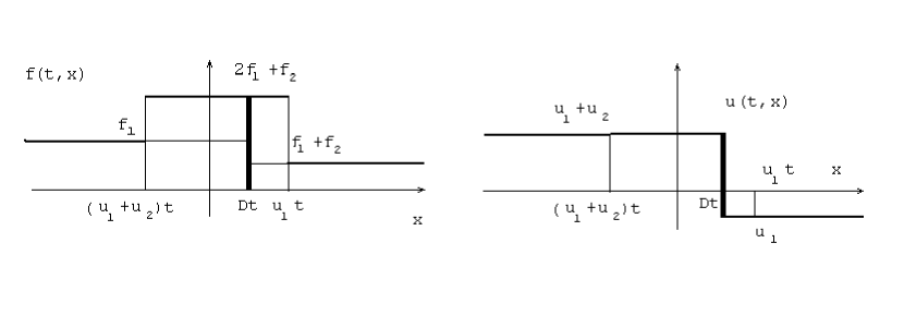
Refer to caption

Figure 4. Changing the noninteracting particles model to the sticky particles model.

The formulas describing the amplitude of the delta-function in the density component and the singularity position obtained earlier in [19],[16],[12] give the same result. Moreover, our method allows to find the jump position in a unique way (in contrast to the method used in [12]).

It is worth mentioning that the spurious pressure (49) does not arise in the sticky particles model.

Remark 8.

The case of the singular Riemann problem with f30subscript𝑓30f_{3}\neq 0 is in fact more different from the case of the regular Riemann problem than it seems at first glance. Let us begin with the constant initial density ([f]=0delimited-[]𝑓0[f]=0), when the trajectory satisfies (52). It is natural to set the amplitude of the initial δ𝛿\delta – function f3subscript𝑓3f_{3} greater or equal than zero. Then the trajectory x(t)𝑥𝑡x(t) is continuous since the denominator in (52) does not vanish. However, if we take f3<0,subscript𝑓30f_{3}<0, then the trajectory goes to infinity at the finite moment where m(t)𝑚𝑡m(t) vanishes, and then the trajectory jumps to infinity of the other sign.

Further, if [f]0,delimited-[]𝑓0[f]\neq 0, then we have to use the formula (51). It can be checked that it is possible to find values u1,u2,f1,f2subscript𝑢1subscript𝑢2subscript𝑓1subscript𝑓2u_{1},u_{2},f_{1},f_{2} (for example, u1=1,u2=2,f1=2,f2=1.8formulae-sequencesubscript𝑢11formulae-sequencesubscript𝑢22formulae-sequencesubscript𝑓12subscript𝑓21.8u_{1}=-1,u_{2}=-2,f_{1}=2,f_{2}=-1.8) such that the expression under the square root vanishes within a finite time t.subscript𝑡t_{*}. However, as follows from (50), (51),

m(t)=f32 2[uf]f3t+([uf]2[f][u2f])t2,𝑚𝑡superscriptsubscript𝑓322delimited-[]𝑢𝑓subscript𝑓3𝑡superscriptdelimited-[]𝑢𝑓2delimited-[]𝑓delimited-[]superscript𝑢2𝑓superscript𝑡2m(t)\,=\,\sqrt{f_{3}^{2}\,-\,2\,[uf]\,f_{3}\,t\,+\,([uf]^{2}-[f][u^{2}f])\,t^{2}},\, (53)

therefore within the same time tsubscript𝑡t_{*} the amplitude of the δ𝛿\delta – function becomes zero. Thus, at the moment tsubscript𝑡t_{*} we have to set a new Riemann problem with the jump at the point x(t).𝑥subscript𝑡x(t_{*}).

8.2. Riemann problem with non-constant states

Now we extend formulas (51) and (52) to the case of the Riemann problem with non-constant left and right states:

f0(x)=f1(x)+θ(x)f2(x)+f3δ(x),subscript𝑓0𝑥subscript𝑓1𝑥𝜃𝑥subscript𝑓2𝑥subscript𝑓3𝛿𝑥f_{0}(x)=f_{1}(x)+\theta(x)f_{2}(x)+f_{3}\delta(x), (54)
u0(x)=u1(x)+θ(x)u2(x),subscript𝑢0𝑥subscript𝑢1𝑥𝜃𝑥subscript𝑢2𝑥u_{0}(x)=u_{1}(x)+\theta(x)u_{2}(x), (55)

where u1(x),subscript𝑢1𝑥u_{1}(x), u2(x),subscript𝑢2𝑥u_{2}(x), f1(x),subscript𝑓1𝑥f_{1}(x), f2(x)subscript𝑓2𝑥f_{2}(x) are smooth functions, f3subscript𝑓3f_{3} is a real constant. We restrict ourselves to a situation that is quite similar to the case of constant states. Namely, we assume that for every x𝑥x\in\mathbb{R} and t>0𝑡0t>0 the straight line y=xst𝑦𝑥𝑠𝑡y=\frac{x-s}{t} has at most two common points with the graph of the function y=u0(s),𝑦subscript𝑢0𝑠y=u_{0}(s), moreover, let u20=limx0+u2(x)<0superscriptsubscript𝑢20subscript𝑥limit-from0subscript𝑢2𝑥0u_{2}^{0}=\lim\limits_{x\to 0+}u_{2}(x)<0 and assume that the intersection points s(t,x)subscript𝑠𝑡𝑥s_{-}(t,x) and s+(t,x)subscript𝑠𝑡𝑥s_{+}(t,x) lie on either side of the origin x=0𝑥0x=0 (see Fig.5).

Refer to caption

Figure 5. The overlapping domain in the Riemann problem

So, every point x𝑥x at the moment t>0𝑡0t>0 lies in the overlapping domain

D=[x(t),x+(t)],x(t)=u+t,x+(t)=ut,formulae-sequence𝐷subscript𝑥𝑡subscript𝑥𝑡formulae-sequencesubscript𝑥𝑡subscript𝑢𝑡subscript𝑥𝑡subscript𝑢𝑡\,D\,=\,[x_{-}(t),x_{+}(t)],\quad x_{-}(t)=u_{+}t,\,x_{+}(t)=u_{-}t,

if the line y=xst𝑦𝑥𝑠𝑡y=\frac{x-s}{t} and the graph of y=u0(s)𝑦subscript𝑢0𝑠y=u_{0}(s) have two points of intersection, s(t,x)<0subscript𝑠𝑡𝑥0s_{-}(t,x)<0 and s+(t,x)>0.subscript𝑠𝑡𝑥0s_{+}(t,x)>0. We set ulimx0u1(x)subscript𝑢subscript𝑥limit-from0subscript𝑢1𝑥u_{-}\,\equiv\,\lim\limits_{x\to 0-}\,u_{1}(x) and u+u+u20.subscript𝑢subscript𝑢superscriptsubscript𝑢20u_{+}\,\equiv\,u_{-}+u_{2}^{0}. Further, we assume that for any fixed t𝑡t the number K𝐾K of points x¯k(t)Dsubscript¯𝑥𝑘𝑡𝐷\bar{x}_{k}(t)\in D such that the straight line and the graph of the initial velocity have a common linear segment is finite. Let us again denote by xj(t)subscript𝑥𝑗𝑡x_{j}(t) the position of the singularity that should change the overlapping domain D𝐷D in the sticky particles model. Then the conservation of mass gives

m(t)=u+txj(t)f(s+(t,x))𝑑x+xj(t)utf(s(t,x))𝑑x+k=1KAk(t,x¯k(t))+f3,𝑚𝑡superscriptsubscriptsubscript𝑢𝑡subscript𝑥𝑗𝑡𝑓subscript𝑠𝑡𝑥differential-d𝑥superscriptsubscriptsubscript𝑥𝑗𝑡subscript𝑢𝑡𝑓subscript𝑠𝑡𝑥differential-d𝑥superscriptsubscript𝑘1𝐾subscript𝐴𝑘𝑡subscript¯𝑥𝑘𝑡subscript𝑓3m(t)\,=\,\int\limits_{u_{+}t}^{x_{j}(t)}\,f(s_{+}(t,x))\,dx\,+\,\int\limits_{x_{j}(t)}^{u_{-}t}\,f(s_{-}(t,x))\,dx\,+\,\sum\limits_{k=1}^{K}\,A_{k}(t,\bar{x}_{k}(t))\,+\,f_{3}, (56)

where Ak(t,x¯k(t))subscript𝐴𝑘𝑡subscript¯𝑥𝑘𝑡\,A_{k}(t,\bar{x}_{k}(t))\, is the amplitude of the δ𝛿\delta – function formed at the point x¯k(t),subscript¯𝑥𝑘𝑡\bar{x}_{k}(t), calculated by using the formula (47).

Further, from the conservation of momentum we have

m(t)x˙j(t)=u+txj(t)f(s+(t,x))u(s+(t,x))𝑑x+xj(t)utf(s(t,x))u(s(t,x))𝑑x+𝑚𝑡subscript˙𝑥𝑗𝑡superscriptsubscriptsubscript𝑢𝑡subscript𝑥𝑗𝑡𝑓subscript𝑠𝑡𝑥𝑢subscript𝑠𝑡𝑥differential-d𝑥limit-fromsuperscriptsubscriptsubscript𝑥𝑗𝑡subscript𝑢𝑡𝑓subscript𝑠𝑡𝑥𝑢subscript𝑠𝑡𝑥differential-d𝑥\displaystyle m(t)\,\dot{x}_{j}(t)\,=\,\int\limits_{u_{+}t}^{x_{j}(t)}\,f(s_{+}(t,x))\,u(s_{+}(t,x))\,dx\,+\,\int\limits_{x_{j}(t)}^{u_{-}t}\,f(s_{-}(t,x))\,u(s_{-}(t,x))\,dx\,+\, (57)
+k=1KAk(t,x¯k(t))ddtx¯k(t),superscriptsubscript𝑘1𝐾subscript𝐴𝑘𝑡subscript¯𝑥𝑘𝑡𝑑𝑑𝑡subscript¯𝑥𝑘𝑡+\,\sum\limits_{k=1}^{K}\,A_{k}(t,\bar{x}_{k}(t))\,\dfrac{d}{dt}\bar{x}_{k}(t),

moreover, the velocity ddtx¯k(t)𝑑𝑑𝑡subscript¯𝑥𝑘𝑡\dfrac{d}{dt}\bar{x}_{k}(t) can be found by the formula

ddtx¯k(t)=u0(s(t,x¯k(t))),𝑑𝑑𝑡subscript¯𝑥𝑘𝑡subscript𝑢0subscript𝑠𝑡subscript¯𝑥𝑘𝑡\dfrac{d}{dt}\bar{x}_{k}(t)\,=\,u_{0}(s_{*}(t,\bar{x}_{k}(t))),

where s(t,x¯k(t))subscript𝑠𝑡subscript¯𝑥𝑘𝑡s_{*}(t,\bar{x}_{k}(t)) is the coordinate of the point where the graph of y=u0(s)𝑦subscript𝑢0𝑠y=u_{0}(s) and the line y=xst𝑦𝑥𝑠𝑡y=\frac{x-s}{t} have a common linear segment. If the graph of y=u0(s)𝑦subscript𝑢0𝑠y=u_{0}(s) does not contain any linear segments, then the respective parts in formulas (56) and (57) vanish. Thus, it is sufficient to substitute (56) into (57) to get the integro-differential equation that governs the singularity position. This equation should be considered together with the initial condition xj(0)=0.subscript𝑥𝑗00x_{j}(0)=0.

8.3. Evolution of the singularity formed from smooth data

As we have seen in Sec.6, if at a point x𝑥x and a moment of time tsubscript𝑡t_{*} starting from smooth initial data loses its smoothness, then there arises a gradient catastrophe in the velocity component (the derivative becomes unbounded), whereas in the density component there arises a δ𝛿\delta – singularity. In the framework of the pressureless gas dynamics for t>t𝑡subscript𝑡t>t_{*} the δ𝛿\delta – singularities encompass the overlapping domain D𝐷D and in the overlapping domain the spurious pressure (given by the integral term discussed in Sec.7) appears. In the sticky particles model we have to collapse the overlapping domain to the one point, where the whole mass of D𝐷D accumulates. The position of this new singularity should be found based on the conservation of mass and momentum.

For the sake of simplicity we assume that every straight line y=xst𝑦𝑥𝑠𝑡y=\frac{x-s}{t} intersects the graph of the smooth initial velocity y=u0(s)𝑦subscript𝑢0𝑠y=u_{0}(s) at most three times. For every fixed x𝑥x initially the intersection point is unique (0<t<t0𝑡subscript𝑡0<t<t_{*}), then at the moment t=t𝑡subscript𝑡t=t_{*} the straight line becomes tangent to the graph of the initial velocity in a certain point, and for t>t𝑡subscript𝑡t>t_{*} we have three intersection points. Our aim is to find the position of the singularity and the amplitude of the δ𝛿\delta – function in the density component.

We denote as before by x(t)subscript𝑥𝑡x_{-}(t) and x+(t)subscript𝑥𝑡x_{+}(t) the endpoints of the domain D,𝐷D, xj(t)subscript𝑥𝑗𝑡x_{j}(t) – the position of the new singularity, A(x(t))𝐴subscript𝑥𝑡A(x_{-}(t)) and A(x+(t))𝐴subscript𝑥𝑡A(x_{+}(t)) – the amplitude of δ𝛿\delta– functions produced at the point where the graphs of y=u0(s)𝑦subscript𝑢0𝑠y=u_{0}(s) and y=x±(t)st𝑦subscript𝑥plus-or-minus𝑡𝑠𝑡y=\frac{x_{\pm}(t)-s}{t} have a common linear segment (for fixed tt𝑡subscript𝑡t\geq t_{*}). Further, let s(t,x),subscript𝑠𝑡𝑥s_{-}(t,x), s0(t,x),subscript𝑠0𝑡𝑥s_{0}(t,x), s+(t,x)subscript𝑠𝑡𝑥s_{+}(t,x) be the subsequent point of intersection (s<s0<s+.subscript𝑠subscript𝑠0subscript𝑠s_{-}<s_{0}<s_{+}.) Let m(t)𝑚𝑡m(t) be the amplitude of the δ𝛿\delta - function in the density component.

Then, the conservation of mass gives

m(t)=A(x(t))+A(x+(t))+𝑚𝑡𝐴subscript𝑥𝑡limit-from𝐴subscript𝑥𝑡m(t)\,=\,A(x_{-}(t))\,+\,A(x_{+}(t))\,+ (58)
x(t)xj(t)(f(s+(t,x))+f(s0(t,x))dx+xj(t)x+(t)(f(s(t,x))+f(s0(t,x))dx,\,\int_{x_{-}(t)}^{x_{j}(t)}\,(f(s_{+}(t,x))\,+\,f(s_{0}(t,x))\,dx\,+\,\int_{x_{j}(t)}^{x_{+}(t)}\,(f(s_{-}(t,x))\,+\,f(s_{0}(t,x))\,dx,

where A(x±(t))𝐴subscript𝑥plus-or-minus𝑡A(x_{\pm}(t)) ca be found by formula (47).

From the conservation of momentum analogously to (57) we have

m(t)x˙j(t)=x(t)xj(t)(f(s+(t,x))u(s+(t,x))+f(s0(t,x))u(s0(t,x)))𝑑x+𝑚𝑡subscript˙𝑥𝑗𝑡limit-fromsuperscriptsubscriptsubscript𝑥𝑡subscript𝑥𝑗𝑡𝑓subscript𝑠𝑡𝑥𝑢subscript𝑠𝑡𝑥𝑓subscript𝑠0𝑡𝑥𝑢subscript𝑠0𝑡𝑥differential-d𝑥\displaystyle m(t)\,\dot{x}_{j}(t)\,=\,\int\limits_{x_{-}(t)}^{x_{j}(t)}\,\big{(}f(s_{+}(t,x))\,u(s_{+}(t,x))+f(s_{0}(t,x))\,u(s_{0}(t,x))\big{)}\,dx\,+ (59)
xj(t)x+(t)(f(s(t,x))u(s(t,x))+f(s0(t,x))u(s0(t,x)))𝑑x+limit-fromsuperscriptsubscriptsubscript𝑥𝑗𝑡subscript𝑥𝑡𝑓subscript𝑠𝑡𝑥𝑢subscript𝑠𝑡𝑥𝑓subscript𝑠0𝑡𝑥𝑢subscript𝑠0𝑡𝑥differential-d𝑥\,\int\limits_{x_{j}(t)}^{x_{+}(t)}\,\big{(}f(s_{-}(t,x))\,u(s_{-}(t,x))+f(s_{0}(t,x))\,u(s_{0}(t,x))\big{)}\,dx\,+\,
A(x(t))u0(s(t,x(t)))+A(x+(t))u0(s+(t,x+(t))).𝐴subscript𝑥𝑡subscript𝑢0subscript𝑠𝑡subscript𝑥𝑡𝐴subscript𝑥𝑡subscript𝑢0subscript𝑠𝑡subscript𝑥𝑡\,A(x_{-}(t))\,u_{0}(s_{-}(t,x_{-}(t)))\,+\,A(x_{+}(t))\,u_{0}(s_{+}(t,x_{+}(t))).

Thus, equations (58), (59) and the initial conditions m(t)=A(x(t)),𝑚subscript𝑡𝐴subscript𝑥subscript𝑡m(t_{*})=A(x_{*}(t_{*})), xj(t)=xsubscript𝑥𝑗subscript𝑡subscript𝑥x_{j}(t_{*})=x_{*} define the position and the amplitude of the singularity of the δ𝛿\delta - function in the component of density. Here xsubscript𝑥x_{*} is a point such that y=xst𝑦subscript𝑥𝑠subscript𝑡y=\frac{x_{*}-s}{t_{*}} and y=u0(s)𝑦subscript𝑢0𝑠y=u_{0}(s) have a common point ssubscript𝑠s_{*} or a common linear segment [s,s+]subscript𝑠subscript𝑠[s_{-},s_{+}] such that the derivatives of both functions are equal at ssubscript𝑠s_{*} or on [s,s+]subscript𝑠subscript𝑠[s_{-},s_{+}] , A(x)𝐴subscript𝑥A(x_{*}) is defined in the statement of Theorem 2.

Remark 9.

If we want to consider the global evolution of the solution to the Burgers equation itself, we should set f0=const.subscript𝑓0constf_{0}=\rm const. The continuity equation plays here an auxiliary role. We are not interested in the properties of the density f,𝑓f, which is constant everywhere except for domains of vacuum and except for the points giving rise to the δ𝛿\delta - singularity.

9. Extension to more general scalar conservation law

Let us consider the following equation

tv+(G(v),)v=0,subscript𝑡𝑣𝐺𝑣𝑣0\partial_{t}v+(G(v),\nabla)v=0, (60)

subject to initial data v(x,0)=v0(x),𝑣𝑥0subscript𝑣0𝑥v(x,0)=v_{0}(x), where v(x,t)=(v1,,vn)𝑣𝑥𝑡subscript𝑣1subscript𝑣𝑛v(x,t)=(v_{1},...,v_{n}) is a vector-function n+1n,superscript𝑛1superscript𝑛\mathbb{R}^{n+1}\rightarrow\mathbb{R}^{n}, G(v)𝐺𝑣G(v) is a non-degenerate differential mapping from nsuperscript𝑛{\mathbb{R}}^{n}\, to n,superscript𝑛\,{\mathbb{R}}^{n}, such that its Jacobian satisfies detGi(v)vj0,detsubscript𝐺𝑖𝑣subscript𝑣𝑗0{\rm det}\frac{\partial G_{i}(v)}{\partial v_{j}}\neq 0, i,j=1,,n.formulae-sequence𝑖𝑗1𝑛i,j=1,...,n.

We can multiply (60) by Gi(v),i=1,,n,formulae-sequencesubscript𝐺𝑖𝑣𝑖1𝑛\nabla G_{i}(v),\,i=1,...,n, to get

tG(v)+(G(v),)G(v)=0.subscript𝑡𝐺𝑣𝐺𝑣𝐺𝑣0\partial_{t}G(v)+(G(v),\nabla)G(v)=0. (61)

Thus, we can introduce a new vectorial variable u=G(v)𝑢𝐺𝑣u=G(v) to reduce the Cauchy problem for (61) to (3) with u0(x)=G(v0(x)).subscript𝑢0𝑥𝐺subscript𝑣0𝑥u_{0}(x)=G(v_{0}(x)). The stochastic perturbation for (61) is (5) with U𝑈U replaced by G(V).𝐺𝑉G(V).

Therefore we find the representation of the solution to the stochastically perturbed along the characteristics of equation (61) using the formula (13) with G(v0(x))𝐺subscript𝑣0𝑥G(v_{0}(x)) instead of u0(x).subscript𝑢0𝑥u_{0}(x).

Thus, we can apply the results obtained in the previous sections to the investigation of the Riemann problem and the arising of singularities for the following analogue of the pressureless gas dynamics system:

gt+divx(gG(v))=0,(gG(v))t+x(gvG(v))=0,formulae-sequencesubscript𝑔𝑡subscriptdiv𝑥𝑔𝐺𝑣0subscript𝑔𝐺𝑣𝑡subscript𝑥tensor-product𝑔𝑣𝐺𝑣0g_{t}+{\rm div}_{x}(gG(v))=0,\quad(gG(v))_{t}\,+\,\nabla_{x}(g\,v\,\otimes\,G(v))=0, (62)

where g(t,x)𝑔𝑡𝑥g(t,x) is a scalar function that can be interpreted as a density.

Thus, just as we relate with the non-viscous Burgers equation the system of pressureless gas dynamics, so also with the equation (60) one can relate the system (62).

To obtain the solution to the Cauchy problem for (60) itself we have to consider the solution to the Cauchy problem for (62) with the data (g0,G(v0)),g0constsubscript𝑔0𝐺subscript𝑣0subscript𝑔0const(g_{0},\,G(v_{0})),\,g_{0}\equiv{\rm const} and then perform the inverse transform v(t,x)=G1(u(t,x)).𝑣𝑡𝑥superscript𝐺1𝑢𝑡𝑥v(t,x)=G^{-1}(u(t,x)).

10. Conclusion

1. Let us notice that the solution of the Riemann problem for the pressureless gas dynamics system obtained in this paper for the 1D case satisfies the entropy condition

u(t,x2)u(t,x1)x2x11t,𝑢𝑡subscript𝑥2𝑢𝑡subscript𝑥1subscript𝑥2subscript𝑥11𝑡\frac{u(t,x_{2})-u(t,x_{1})}{x_{2}-x_{1}}\,\leq\,\frac{1}{t}, (63)

for any sufficiently small x1subscript𝑥1x_{1} and x2subscript𝑥2x_{2} (e.g.[19]) and the balance relations on the jump that the definition of solution in the sense of integral identity implies ([16]) are satisfied as well. It is known that these conditions do not guarantee uniqueness ([19], [12]). However, our solution is unique both in the case of rarefaction and compression. In the case of rarefaction it is automatically self-similar (we recall that the assumption of the self-similarity implies uniqueness [29]). In the case of contraction the problem of uniqueness was open for the solution to the singular Riemann problem, where a non-zero mass is concentrated on the jump at the initial time. As was noticed in [12], for the uniqueness one must prescribe the derivative of the amplitude of the δ𝛿\delta - function. In our framework the solution is unique and the value of the derivative of the amplitude of the δ𝛿\delta - function follows from the expression for the amplitude itself.

2. In [17] an analog of the system (19), (20) (without the integral term) in the 1D case was obtained. Namely, it was proved that for smooth initial data a local in time strong solution (ρ(t,x),u(t,x))𝜌𝑡𝑥𝑢𝑡𝑥(\rho(t,x),\,u(t,x)) to this system can be constructed by means of a nonlinear diffusion process

Xt=X0+0t𝔼[(u0(X0))|Xs]𝑑s+σWt,(X0)=ρ(0,x),formulae-sequencesubscript𝑋𝑡subscript𝑋0superscriptsubscript0𝑡𝔼delimited-[]conditionalsubscript𝑢0subscript𝑋0subscript𝑋𝑠differential-d𝑠𝜎subscript𝑊𝑡subscript𝑋0𝜌0𝑥X_{t}=X_{0}+\int\limits_{0}^{t}\,\mathbb{E}[(u_{0}(X_{0}))|X_{s}]\,ds\,+\,\sigma W_{t},\quad\mathcal{L}(X_{0})=\rho(0,x),

so that ρ(t,x)𝜌𝑡𝑥\rho(t,x) is the probability density of the diffusion process Xtsubscript𝑋𝑡X_{t} and u(t,x)=E[(u0(X0))|Xt=x]𝑢𝑡𝑥𝐸delimited-[]conditionalsubscript𝑢0subscript𝑋0subscript𝑋𝑡𝑥u(t,x)=E[(u_{0}(X_{0}))|X_{t}=x] (with E[.,|..]E[.,|\,..] standing for conditional expectation and (X0)subscript𝑋0\,{\mathcal{L}}(X_{0})\, for the probability density of X0subscript𝑋0X_{0}). In fact, this result relates to our Proposition 2, since we have shown that the integral term arises only for discontinuous data.

Further, in [18] the system (19), (20) (without the integral term) was considered in any dimension. In this work there was constructed a global weak solution using discrete approximations, and the interaction of particles is given by a sticky particles dynamics.

3. There exist formalisms to represent solutions of parabolic PDE’s as the expected value of functionals of stochastic processes (see e.g. [22], [23], [3], [5] and references therein). In particular, in [11] one can find a recent result concerning the stochastic formulation of the viscous Burgers equation. An alternative approach to the stochastic formulation for a much more wider class of parabolic equations and systems can be found in [4].

4. We would also like to mention the paper [9], where a numerical method of particles for the solution of the pressureless gas dynamics in 1D an 2D case has been developed. The method is mostly inspired by [20] and in fact in this paper the problem of transition from the non-interacting particles to the sticky particle model was solved numerically.

Acknowledgements We are grateful to Ya.Belopolskaya, V.Danilov, A.Kurganov, E.Panov and V.Shelkovich for fruitful discussions.

References

  • [1] S. Albeverio, O. Rozanova, (2009)  The non-viscous Burgers equation associated with random position in coordinate space: a threshold for blow up behaviour, Mathematical Models and Methods in Applied Sciences, Vol. 19, No. 5, pp. 1-19.
  • [2] S. Albeverio, O.Rozanova (2009)  Suppression of unbounded gradients in SDE associated with the Burgers equation, Proceedings of Amer.Math.Soc..in press.
  • [3] Ya.I.Belopolskaya, Yu.L.Daletskij, (1990) Stochastic equations and differential geometry, Kluwer Academic Publishers.
  • [4] S.Albeverio, Ya.I. Belopolskaya (2005)  Probabilistic Interpretation of the vv-method for PDE Systems, Chapter in the book ”Analytical approaches to multidimensional balance laws” (Olga S. Rozanova ed.), Nova Science Publishers, New York.
  • [5] Ya. Belopolskaya. Burgers equation on a Hilbert manifold and the motion of incompressible fluid. Methods of Functional Analysis and Topology v.5 N4 (1999) 15-27 .
  • [6] Y.Brenier,  E.Grenier, (1998) Sticky particles model and scalar conservation laws SIAM J.Numer.Anal., 35 , 2317 - 2328.
  • [7] N.V. Brilliantov, T.Pöschel (2004)  Kinetic theory of granular gases, Oxford University Press, Oxford.
  • [8] F.Bouchut, F.James,  (1999)  Duality solutions for pressureless gases, monotone scalar conservation laws, and uniqueness, Comm.Partial Differ. Equat., 24 N11-12, pp.2173–2189.
  • [9] A.Chertock, A.Kurganov, Yu.Rykov. (2007) A new skicky particles method for pressureless gas dynamics. SIAM J. Numer.Anal., 35, 2408 - 2441.
  • [10] A.J.Chorin, O.H. Hald,   (2006)  Stochastic tools in mathematics and science, Springer, Berlin.
  • [11] P.Constantin, G.Iyer, (2008)  A stochastic Lagrangian representation of the three-dimensional incompressible Navier-Stokes equations. Commun. Pure Appl. Math. 61 (3) 330-345.
  • [12] V.G.Danilov  (2008)  Remarks on vacuum state and uniqueness of concentration process, Electronic Journal of Diff.Equat., No.34, pp. 1-10.
  • [13] V. Danilov, D. Mitrovic (2005) Weak asymptotics of shock wave formation process. Nonlinear Anal., Theory Methods Appl. 61 , No.4 (A), 613-635.
  • [14] V.Danilov, D.Mitrovic (2008)   Delta shock wave formation in the case of triangular hyperbolic system of conservation laws. J. Differ. Equations 245, No. 12, 3704-3734.
  • [15] V. G.Danilov, Shelkovich, (2005) Dynamics of propagation and interaction of δ𝛿\delta-shock waves in conservation law systems. J. Diff. Equat. 211, 333–381.
  • [16] Danilov V.G., V. M.Shelkovich   (2005)  Delta-shock wave type solution of hyperbolic systems of conservation laws, Quaterly of Applied Mathematics, Vol. 63, pp. 401-427.
  • [17] A.Dermoune, B.Djehiche  (2001)  Pressureless gas equations with viscosity and nonlinear diffusion, CR Acad. Sci. Paris, t.332, Serie 1, pp. 745-750.
  • [18] A. Dermoune, B. Djehiche (2002)  Global solution of the pressureless gas with viscosity , Physica D, 163, pp.184-190.
  • [19] F.Huang, Zh. Wang (2001) Well posedness for pressureless flow. Commun. Math. Phys. 222, No.1, 117-146.
  • [20] Weinan E, Yu.G.Rykov, Ya.G.Sinai  (1996)  Generalized veriational principles, global weak solutions and behavior with random initial data for system of conservation laws arising in adhesion particle dynamics,Commun. Math. Phys, 177, pp.349 – 380.
  • [21] L.C.Evans  (1998)  Partial differential equations, AMS, Providence.
  • [22] M.Freidlin  (1985)  Functional integration and partial differential equations, Annals of Mathematics Studies, No.109 (Princeton, New Jersey: Princeton University Press).
  • [23] M.Freidlin (1996)  Markov processes and differential equations: asymptotic problems, Lectures in Mathematics, (ETH Zu”rich. Basel: Birkha”user).
  • [24] K.T.Joseph  (1993)  A Riemann problem whose viscocity solution contains δ𝛿\delta - measures, Asymptotic Analysis, 7, pp.105-120.
  • [25] H.A.Levine, M.H.Protter  (1986)  The breakdown of solutions of quasilinear first order systems of partial differential equations, Arch.Rat.Mech.Anal., 95, pp.253-267.
  • [26] B.L.Rozhdestvenskij, N.N.Yanenko  (1983)  Systems of quasilinear equations and their applications to gas dynamics, Translations of Mathematical Monographs, Vol. 55, Providence, R.I.: American Mathematical Society (AMS).
  • [27] S.Shandarin, Ya.B.Zeldovich  (1989)  The large structure of the universe: turbulence, intermittence, structures in a self-gravitating medium, Rev.Modern. Phys, Vol. 61, pp. 185-220.
  • [28] V. M.Shelkovich   (2006)  The Rankine-Hugoniot conditions and balance laws for δ𝛿\delta-shock waves. Fundam. Prikl. Mat. 12, no. 6, 213–229 (translation in J. Math. Sci. (N. Y.) 151 (2008), no. 1, 2781–2792).
  • [29] W.Sheng, T.Zhang  (1999)  The Riemann problem for the transport equation in gas dynamics. Mem.Amer.Math.Soc., 654, AMS, Providence.
  • [30] G. N. Watson  (1995)  A Treatise on the Theory of Bessel Functions, Second Edition, Cambridge University Press.