Multinetwork of International Trade:
A Commodity-Specific Analysis

Abstract

We study the topological properties of the multinetwork of commodity-specific trade relations among world countries over the 1992-2003 period, comparing them with those of the aggregate-trade network, known in the literature as the international-trade network (ITN). We show that link-weight distributions of commodity-specific networks are extremely heterogeneous and (quasi) log normality of aggregate link-weight distribution is generated as a sheer outcome of aggregation. Commodity-specific networks also display average connectivity, clustering, and centrality levels very different from their aggregate counterpart. We also find that ITN complete connectivity is mainly achieved through the presence of many weak links that keep commodity-specific networks together and that the correlation structure existing between topological statistics within each single network is fairly robust and mimics that of the aggregate network. Finally, we employ cross-commodity correlations between link weights to build hierarchies of commodities. Our results suggest that on the top of a relatively time-invariant “intrinsic” taxonomy (based on inherent between-commodity similarities), the roles played by different commodities in the ITN have become more and more dissimilar, possibly as the result of an increased trade specialization. Our approach is general and can be used to characterize any multinetwork emerging as a nontrivial aggregation of several interdependent layers.

I Introduction

The past decade has seen an increasing interest in the study of international-trade issues from a complex-network perspective (Li et al., 2003; Serrano and Boguñá, 2003; Garlaschelli and Loffredo, 2004, 2005; Serrano et al., 2007; Bhattacharya et al., 2008, 2007; Garlaschelli et al., 2007; Tzekina et al., 2008; Fagiolo et al., 2008; Reyes et al., 2008; Fagiolo et al., 2009a). Existing contributions have attempted to investigate the time-evolution of the topological properties of the aggregate International Trade Network (ITN), aka the World Trade Web (WTW), defined as the graph of all import/export relationships between world countries in a given year.

Two main approaches have been employed to address this issue. In the first one, the ITN is viewed as a binary graph where a (possibly directed) link is either present or not according to whether the value of the associated trade flow is larger than a given threshold (Serrano and Boguñá, 2003; Garlaschelli and Loffredo, 2004, 2005). In the second one, a weighted-network approach (Barrat et al., 2004; Barthélemy et al., 2005) to the study of the ITN has been used, i.e. links between countries are weighted by the (deflated) value of imports or exports occurred between these countries in a given time interval (Li et al., 2003; Bhattacharya et al., 2008, 2007; Garlaschelli et al., 2007; Fagiolo et al., 2008; Fagiolo et al., 2009a). In most cases, a symmetrized version of the ITN has been studied, where only undirected trade flows are considered and one neglects —in a first approximation— the importance of directionality of trade flows.

Such studies have been highlighting a wealth of fresh stylized facts concerning the architecture of the ITN, how they change through time, how topological properties correlate with country characteristics, and how they are predictive of the likelihood that economic shocks might be transmitted between countries (Kali and Reyes, 2007). However, they all consider the web of world trade among countries at the aggregate level, i.e. links represent total trade irrespective of the commodity actually traded . Here we take a commodity-specific approach and we unfold the aggregate ITN in many layers, each one representing import and export relationships between countries for a given commodity class (defined according to standard classification schemes, see below).

More precisely, we employ data on bilateral trade flows taken from the United Nations Commodity Trade Database to build a multi-network of international trade. A multi-network (Wasserman et al., 1994) is a graph where a finite, constant set of nodes (world countries) are connected by edges of different colors (commodities). Any two countries might then be connected by more than one edge, each edge representing here a commodity-specific flow of imports/exports. As our data span a 12-year interval, $N=162$ countries and $C=97$ commodities, we therefore have a sequence of 12 international-trade multi-networks (ITMNs), where between any pair of the $N$ countries there may be at most $C$ edges. Each ITMN can then be viewed in its entirety or also as the juxtaposition of $C=97$ commodity-specific networks, each modeled as a weighted directed network. We weight a link from country $i$ to $j$ by the (properly rescaled) value of $i$’s exports to $j$, and, in general, the link from $i$ to $j$ is different from the link from $j$ to $i$.

The multi-network setup allows us to ask novel questions related to the structural properties of the ITN. For example: To what extent do topological properties of the aggregate ITN depend on those of the commodity-specific networks? Are trade architectures heterogeneous across commodity-specific networks? How do different topological properties correlate within each commodity-specific network, and how do the same topological property cross-correlates across commodity-specific network? How do countries perform in different commodity-specific networks as far as their topological properties are concerned (i.e. centrality, clustering, etc.)? Is it possible to build correlation-based distances among commodities and build taxonomies that account for “intrinsic” factors (inherent similarity between commodities as described in existing classification schemes) as well as for “revealed” factors (determined by the actual pattern of trades)?

In this paper we begin answering these questions. Our preliminary results show that commodity-specific networks are extremely heterogeneous as far as link-weight distributions are concerned and that the (quasi) log-normality of aggregate link-weight distribution is generated as a sheer outcome of aggregation of statistically dissimilar commodity-specific distributions. Commodity-specific networks also display average connectivity, clustering and centrality levels very different from their aggregate counterparts. We also study the connectivity patterns of commodity-specific networks and find that complete connectivity reached in the aggregate ITN is mainly achieved through the presence of many weak links that keep commodity-specific networks together, whereas strong trade links account for tightly interconnected clubs of countries that trade with each other in all commodity networks. We also show that, despite a strong distributional heterogeneity among commodity-specific link-weight distributions, the correlation structure existing between topological statistics within each single network is fairly robust and mimics that of the aggregate network. Furthermore, we find that cross-commodity correlations of the same statistical property are almost always positive, meaning that on average large values of node clustering and centrality in a commodity network imply large values of that statistic also in all other commodity networks. Finally, we introduce a general method to characterise hierarchical dependencies among layers in multi-networks, and we use it to compute cross-commodity correlations. We exploit these correlations between link weights to explore the possibility of building taxonomies of commodities. Our results suggest that on the top of a relatively time-invariant “intrinsic” taxonomy (based on inherent between-commodity similarities), the roles played by different commodities in the ITN have become more and more dissimilar, possibly as the result of an increased trade specialization.

The rest of the paper is organized as follows. Section II describes the database, explains the methodology employed to build the ITMNs and defines the basic topological statistics employed in the analysis. Sections III and IV report our main results. Concluding remarks are in Section V.

II Data and Definitions

II.1 Data

We employ data on bilateral trade flows taken from the United Nations Commodity Trade Database (UN-COMTRADE; see http://comtrade.un.org/). We build a balanced panel of $N=162$ countries for which we have commodity-specific imports and exports flows from 1992 to 2003 ($T=12$ years) in current U.S. dollars. Trade flows are reported for $C=97$ (2-digit) different commodities, classified according to the Harmonized System 1996 (HS1996; see Table LABEL:Tab:HS and http://www.wcoomd.org/).

II.2 The International-Trade Multi-Network

We employ the database to build a time sequence of weighted, directed multi-networks of trade where the $N$ nodes are world countries and directed links represent the value of exports of a given commodity in each year or wave $t=1992,\dots,2003$. As a result, we have a time sequence of $T$ multi-networks of international trade, each characterized by $C$ layers (or links of $C$ different colors). Each layer $c=1,\dots,C$ represents exports between countries for commodity $c$ and can be characterized by a $N\times N$ weight matrix $X_{t}^{c}$. Its generic entry $x_{ij,t}^{c}$ corresponds to the value of exports of commodity $c$ from country $i$ to country $j$ in year $t$. We consider directed networks, therefore in general $x_{ij,t}^{c}\neq x_{ji,t}^{c}$. The aggregate weighted, directed ITN is obtained by simply summing up all commodity-specific layers. The entries of its weight matrices $X_{t}$ will read:

$$x_{ij,t}=\sum_{c=1}^{C}{x_{ij,t}^{c}}.$$ (1)

In order to compare networks of different commodities at a given time $t$, and to wash-away trend effects, we re-scale all commodity-specific trade flows by the total value of trade for that commodity in each given year. This means that in what follows we shall study the properties of the sequence of international-trade multi-networks (ITMNs) where the generic entry of the weight matrix is defined as:

$$w_{ij,t}^{c}=\frac{x_{ij,t}^{c}}{\sum_{h=1}^{N}\sum_{k=1}^{N}x_{hk,t}^{c}}.$$ (2)

Therefore, the directed $c$-commodity link from country $i$ to country $j$ in year $t$ is weighted by the ratio between exports from $i$ to $j$ of $c$ to total year-$t$ trade of commodity $c$.

Accordingly, the generic entry of the aggregate-ITN weight matrix is re-scaled as:

$$w_{ij,t}=\frac{x_{ij,t}}{\sum_{h=1}^{N}\sum_{k=1}^{N}x_{hk,t}}.$$ (3)

Commodity-specific adjacency (binary) matrices $A_{t}^{c}$ are obtained from weighted ones by simply setting $a_{ij,t}^{c}=1$ if and only if the corresponding weight is larger than a given time- and commodity-specific threshold $\underline{w}_{t}^{c}$. Unless explicitly noticed, we shall set $\underline{w}_{t}^{c}=0$.

Before presenting a preliminary descriptive analysis of the data, two issues are in order. First, most of our analysis below will focus on year 2003 for the sake of simplicity. We employ a panel description in order to keep a fixed-size country network and avoid difficulties related to across-year comparison of topological measures, when required. Of course, accounting for entry/exit of countries in the network may allow one to explore hot issues in international trade literature as the relative importance of intensive and extensive margins of trade from a commodity specific approach (Hummels and Klenow, 2005; De Benedictis and Tajoli, 2008). Although all our results seem to be reasonably robust in alternative years, a more thorough comparative-dynamic analysis is the next point in our agenda. Second, in order to correctly account for trend effects, one should deflate commodity-specific trade flows by its industry-specific deflator, which unfortunately is not available for all countries. That is why we have chosen to remove trend effects and scale trade flows by total commodity-specific trade in that year.

II.3 Commodity Space

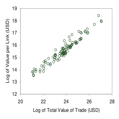
One of the aims of the paper, as mentioned, is to assess the across-commodity heterogeneity of commodity-specific networks in terms of their topological properties, as compared to those of the aggregate network. For the sake of exposition, we shall focus, when necessary, on the most important commodity networks. Table 2 shows the ten most-traded commodities in 2003, ranked according to the total value of trade. Notice that they account, together, for 56% of total world trade and that the 10 most-traded commodities feature also the highest values of trade-value per link (i.e. ratio between total trade and total number of links in the commodity-specific network). Indeed, total trade value and trade-value per link of commodities are positively correlated (see Figure 2), as are total-trade value and network density (with a correlation coefficient of 0.52). In addition to those trade-relevant 10 commodities, we shall also focus on other 4 classes (cereals, cotton, coffee/tea and arms), which are less traded but more relevant in economics terms. The 14 commodities considered account together for 57% of world trade in 2003.

II.4 Topological Properties

In the analysis below we shall focus on the following topological measures to characterize trade networks and to compare them across commodities:

• Density (d): Network density is defined as the share of existing to maximum possible links in the binary $N\times N$ matrix.

• Node in-degree ($ND_{in}$) and out-degree ($ND_{out}$): measure the number of countries from (respectively, to) which a given node imports (respectively, exports).

• Node in-strength ($NS_{in}$) and out-strength ($NS_{out}$): Account for the share of country’s total imports (respectively, exports) to world total commodity trade; more generally, in-strength (respectively, out-strength) is defined as the sum of all weights associated to inward (respectively, outward) links of a node. Node strength (NS) is simply defined as the sum of $NS_{in}$ and $NS_{out}$. Interesting statistics are also the ratios $NS_{in}/ND_{in}$ (average share of import per import partner) and $NS_{out}/ND_{out}$ (average share of export per export partner).

• Node average nearest-neighbor strength (ANNS): measures the average NS of all the partners of a node. ANNS can be declined in four different ways, according to which one only considers the average $NS_{in}$ or $NS_{out}$ of import or export partners. Hence, $ANNS_{in-out}$ (respectively, $ANNS_{in-in}$) account for the average values of exports (respectively, imports) of countries from which a given node imports; similarly, $ANNS_{out-in}$ (respectively, $ANNS_{out-out}$) represent the average values of imports (respectively, exports) of countries to which a given node exports;

• Node weighted clustering coefficient ($WCC_{all}$): proxies the intensity of trade triangles with that node as a vertex, where each edge of the triangle is weighted by its link weight (Saramaki et al., 2007). In weighted directed networks, one might differentiate across four types of directed triangles and compute four different types of clustering coefficients (Fagiolo, 2007): (i) $WCC_{mid}$, measuring the intensity of trade triangles where node $i$ (the middleman) imports from $j$ and exports to $h$, which in turn imports from $j$; (ii) $WCC_{cyc}$, measuring the intensity of trade triangles where nodes $i$, $j$ and $h$ create a cycle; (iii) $WCC_{in}$, accounting for triangles where node $i$ imports from both $j$ and $h$; and (iv) $WCC_{out}$, accounting for triangles where node $i$ exports to both $j$ and $h$.

• Node weighted centrality (WCENTR): measures the importance of a node in a network. Among the many suggested measures of node centrality (Koschützki et al., 2004), we employ here a version of Bonacich eigenvector-centrality suited to weighted-directed networks (Bonacich and Lloyd, 2001). It assigns relative scores to all nodes in the network based on the principle that connections to high-scoring nodes contribute more to the score of the node in question than equal connections to low-scoring nodes.

In addition to the above topological statistics, we also study the distributions of link weights (both across commodity networks and in the aggregate). Finally, we shall explore patterns of binary connectivity by studying the properties (e.g. size and composition ) of the largest connected component .

III Topological Properties of Commodity-Specific Networks

III.1 Commodity-specific sample moments of topological properties

We begin with a comparison of sample moments (mean and standard deviation) of the relevant link and node statistics across different commodities. We compare sample moments to those of the aggregate network to assess the degree of heterogeneity of commodity networks and single out those that behave excessively differently from the aggregate counterpart.

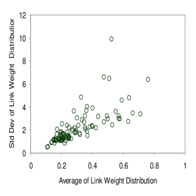
Table 3 reports the density of the 14 most relevant commodities, together with the mean and standard deviation of a few link-weight and node-statistic distributions as described in Section II.4. Notice that, as compared to the aggregate network, all commodity-specific networks display larger average link weights, shares of export/link and import/link, as well as overall clustering. This means that connectivity and clustering patterns of the commodity-specific trade networks are more intense than their aggregate counterpart once one washes away the relative composition of world trade. Conversely, by definition, all commodity-specific densities are smaller than in the aggregate. Among the 14 most relevant commodities, however, there appears to be a marked heterogeneity. For example, arms (code 93) display a relatively low density but a very strong average link weight and the largest import and export per link shares and clustering. Cereals, on the other hand, display a relatively small density as compared to the aggregate, but exhibit a very large average link weight and shares of import per inward link. The latter is larger than the average shares of export per outward link, a result that generalizes for almost all commodity-specific networks, see Figure 2. Larger shares of exports per outward link are associated to larger shares of imports per inward link, but the relative weight of imports dominates. This means that on average countries tend to have, irrespective of the commodity traded and its share on world market, more intensive import relations than export ones (see also subsection III.5).

Another fairly general evidence regards the scaling between average and standard deviation in link and node distributions. There appears to be a positive relation between average and standard deviation of node and link statistics (see Figure 3 for the example of link weights), suggesting that within each commodity-specific network larger trade intensities and clustering levels are gained at the expense of a much strong heterogeneity in the country-distributions of such topological features.

To conclude this preliminary analysis, we report some results on the directed clustering patterns observed across commodity networks. Following (Fagiolo, 2007), we compute the percentage of directed trade triangles of different types that each country forms with their partners (see Table 4). Note that in the aggregate network there is a slight preponderance of out-type triangles (patterns where a country exports to two countries that are themselves trade partners). Conversely, commodity-specific networks are characterized also by a large fraction of in-type clustering patterns (a country importing from two countries that are themselves trade partners),except coffee and precious metals for which out-type clustering is more frequent. The other two types of clustering patterns (cycle and middlemen) are much less frequent.

III.2 Distributional Features of Topological Properties

The foregoing results on average-dispersion scaling and heterogeneity across commodity networks suggests that the overall evidence on aggregate trade topology may be the result of extremely heterogeneous networks. For example, previous studies on other data (Fagiolo et al., 2009a; Gleditsch, 2002) have highlighted the pervasiveness of log-normal shapes as satisfactory proxies to describe the link- and node-distributions of aggregate link-weights, strength, clustering and so on, in symmetrized versions of the ITN. Only node centrality measures (computed using the notion of random-walk betweenness centrality, see Ref. (Fisher and Vega-Redondo, 2006)) seemed to display power-law shaped behavior.

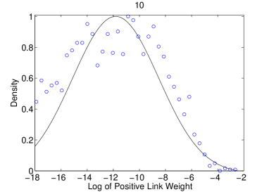
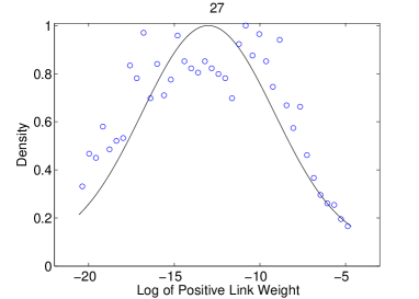
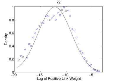
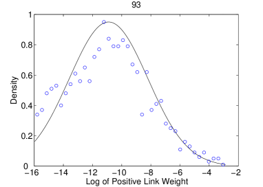
To begin exploring the issue whether log-normal aggregate distributions are the result of heterogeneous, possibly non log-normal, commodity-specific distributions, we have run a series of goodness-of-fit exercises to test whether: (i) any two pairs of commodity-specific networks are characterized by the same link-weight distribution; (ii) commodity-specific link-weight distributions are log-normal (i.e., logs of their positive values are normal). Our result show that the body of the aggregate distribution can be well-proxied by a log-normal, whereas the upper tail seems to be thinner than what expected under log-normality (less high-intensity links as expected). This means that log-normality found by (Fagiolo et al., 2009a) may be also the outcome of symmetrization, i.e. of studying a undirected weighted version of the ITN. We also find that only in 4% of all the possible pairs of distributions ($4656=97*96/2$), the p-value of the associated two-sided Kolmogorov test is greater than 5%. These implies that link-weight distributions are extremely heterogeneous across commodities. Furthermore, according to both Lilliefors and one-sample normality Kolmogorov tests, the majority of distributions seem to be far from log-normal densities, see Figure 4 for some examples. This suggests that the outcome of quasi-log-normality of link weights of the overall network may be a sheer outcome of aggregation.

III.3 Connected Components

We now turn to analyzing the connectivity patterns of the binary aggregate and commodity-specific trade networks by studying the size and composition of their largest connected components.

If we employ the weaker definition of connectivity between two nodes in a directed graph (either an inward or an outward link in place), then the aggregate ITN is fully connected, i.e. the largest connected component (LCC) contains all $N$ countries. If we instead use the stronger definition (both the inward or the outward link in place), then the aggregate network is never completely connected in the time interval under analysis, and the composition of the LCC changes with time. Table 5 shows the percentage size of the LCC for the aggregate network, disaggregated according to geographical macro-areas (i.e., we only consider the LCC in the sub-network of the aggregate ITN made only of countries belonging to any given geographical macro area). In Europe trade links are almost always reciprocated and we notice the fast integration of Eastern Europe after the mid 90s. Sub-Saharan Africa is the area where we find the majority of countries without bilateral trade with other countries of the area, a sign of poor trade connectivity perhaps related to wars, trade barriers, lack of infrastructures, etc..

It is interesting to compare the above considerations about the reciprocity structure of the international trade network with a series of results Garlaschelli and Loffredo (2004, 2005) performed on a different dataset reporting aggregate trade over the longer period 1950-2000 Gleditsch (2002). Those analyses reveal that the reciprocity has been fluctuating about an approximately constant value up to the early 80 s, and has then been increasing steadily. In other words, the international trade system appears to have undergone a rapid reciprocation process starting from the 80 s. At the same time, the fraction of pairs of countries trading in any direction (i.e. the density of the network when all links are regarded as undirected) displays a constant trend over the same period. Therefore, while at an undirected level there is no increase of link density, at a directed level there is a steep increase of reciprocity. The combination of these results signals many new directed links being placed between countries that had already been trading in the opposite direction, rather than new pairs of reciprocal links being placed between previously noninteracting countries. Thus, at an aggregate level many pairs of countries that had previously been trading only in a single direction have been establishing also a reverse trade channel, and this effect dominates on the formation of new bidirectional relationships between previously non-trading countries.

We turn now to analyze connectivity patterns of commodity-specific networks. In this case, it is more reasonable to assume that two countries are connected in a given commodity-specific network if they are linked either by an import or export relationship (the weaker assumption above). Unlike the aggregate network, no commodity-specific graph is completely connected. In what follows, for the sake of exposition, we focus on year 2003 and we report connectivity results for our 14 top commodities. Table 6 reports the size of the LCC in different setups as far as the threshold $\underline{w}_{t}^{c}$ for the determination of binary relationships is concerned ($\underline{w}_{t}^{c}=0$, $\underline{w}_{t}^{c}=w_{t}^{c,p}$, where $w_{t}^{c,p}$ is the p-th percentile of the link-weight distribution, with $p=90\%,95\%,99\%$). When all trade fluxes are considered in the determination of a binary link, then all commodity-specific networks are highly connected, and the size of the LCC is relatively close to network size (except for the case of arms). If one raises the lower threshold and only considers the 10%, 5% and 1% strongest link weights in each matrix, then few countries remain connected. For each commodity, Table 7 lists the countries belonging to the LCC in year 2003 and for the strongest 1% links. It is easy to see that the “usual suspects” (USA, Germany, Japan, etc.) belong to almost all commodity LCCs. Some of them are unexpectedly small (coffee, cereals), others are very large even if one is only focusing on a few largest trade links. All in all, this evidence indicates that complete connectivity in the ITN is mainly achieved through weak links, whereas strong links account for tightly interconnected clubs that trade with each other not only in the aggregate but also every possible commodity.

III.4 Country rankings

In this subsection we analyze country rankings in 2003 according to the alternative topological properties studied in the paper. For each node statistic, we rank in a decreasing order countries in the panel and we report the top-3 positions for our 14 benchmark commodities, as well as for the aggregate network. Results are in Tables 8–10.

As far as node strength is concerned, USA, Germany, China and UK exhibit top values of both import shares and output shares in almost all commodity networks. These are the countries that trade more irrespective of the specific commodity. Russia, Saudi Arabia and Norway top the fuel export ranking, Brazil excels in coffee export, whereas Hong Kong and Mexico enter the top-3 positions in cotton and cereals, respectively. ANNS rankings (Table 9) are more instructive, because they reveal that countries trading with partners that imports/exports more, are typically small economies located outside Europe and North America. This points to a general disassortative structure of the network also at the commodity-specific level, a structural pattern that has been observed in the aggregate as well in previous studies (Garlaschelli and Loffredo, 2004; Fagiolo et al., 2008).

Rankings of clustering, on the other hand, display a markedly-larger commodity heterogeneity in terms of countries appearing in the top-3 positions. Table 10 shows results about overall weighted clustering, i.e. the relative intensity of trade triangles with the target country as a vertex, irrespective of the direction of trade flows. Notice that in the aggregate USA, Germany and China are the most clustered nodes, but they do not always show up in the same positions in all commodity rankings. This means that they typically form extremely strong triangles in a few commodity networks (e.g., for USA pharmaceutical, optical instruments). Note also the high-clustering levels reached by Colombia in coffee trade, Algeria in cereals, Equatorial Guinea in mineral fuels and organic chemicals, Uzbekistan in cotton. These are countries that tend to be involved with a relevant intensity only in one particular type of trade triangle, e.g. in-type for Algeria, out-type for Equatorial Guinea, Uzbekistan and Colombia. This suggests, for example, that Algeria is very likely to import cereals from two countries that are also trading cereals very much. Similarly, Equatorial Guinea, Uzbekistan and Colombia tend to intensively export mineral fuels, cotton and coffee, respectively, to pairs of countries that also trade intensively these commodities together. Finally, centrality rankings shed some light on the relative positional importance of countries in the network. Rankings stress, beside the usual list of large and influential countries, the key role played by Switzerland in precious metals, Russia, Saudi Arabia and Norway in mineral fuels, Indonesia in coffee and Thailand in cereals.

III.5 Correlations between topological properties within commodity networks

Early work on the aggregate ITN has singled out robust evidence about the correlation structure between topological properties (Garlaschelli and Loffredo, 2004, 2005; Garlaschelli et al., 2007; Fagiolo et al., 2008; Fagiolo et al., 2009a, b). For example, disassortative patterns (negative correlation between ANND/ND and ANNS/NS; see also above) has been shown to characterize the binary ITN (strongly) and the weighted ITN (weakly). Also, the aggregate ITN exhibits a trade structure where countries that trade more intensively are more clustered and central. Here we check whether such structure is robust to disaggregation at the commodity level by comparing the correlation between different topological properties (e.g., $NS_{in}$ vs. $ND_{in}$) within each commodity network. In the next section, conversely, we shall look at how the same topological property (e.g., $NS_{in}$) correlates across different networks.

Table 11 shows the most interesting correlation coefficients between node statistics . Note first that, all in all, the sign of any given correlation coefficient computed for the aggregate network remains the same across almost all commodity-specific networks. This is an interesting robustness property, as we have shown that commodity-specific networks are relatively heterogeneous according to e.g. the shape of their link-weight distribution. It appears instead that despite heterogeneously-distributed link weights the inherent architecture of commodity-specific networks mimics those of the aggregate (or viceversa).

Almost all the signs are in line with what previously observed. For example, countries that trade with more partners also trade more intensively (both as exporters ad importers). Furthermore, countries that import (export) more, typically import from (export to) countries that in turn export on average relatively less (disassortativity). The magnitude of this disassortativity pattern is however different according to whether one looks at imports of exports. On average, countries that import from a given country, trade relatively less than those that export to the same country, i.e. the magnitude of the correlation coefficients between $NS_{out}$ and both $ANNS_{out-in}$ and $ANNS_{out-out}$ is larger than the magnitude of the correlation coefficients between $NS_{in}$ and both $ANNS_{in-in}$ and $ANNS_{in-out}$.

Another robust correlation pattern that emerges is about clustering and centrality. Countries that trade more in terms of their node strengths are also more clustered and more central. This happens irrespectively of the commodity traded.

The only partial exceptions to such evidence are represented by the commodity networks of cereals and mineral fuels. For example, countries that imports relatively more cereals (mineral fuels) typically import from countries that also export (import) more cereals (mineral fuels). This does not happen however for exports of such commodities, as correlations are negative or very close to zero. Also, countries that trade more these two commodities are relatively less clustered than happens in other commodity classes.

III.6 Correlations between topological properties across commodity networks

In the latter subsection we have investigated correlations computed between different node topology statistics within the same network. We now explore correlation patterns of node statistics across commodity networks. More precisely, for each given node statistic $X$, we compute all possible $C(C-1)/2=4656$ correlation coefficients:

$$\rho^{c,c^{\prime}}(X)=\frac{\sum_{i=1}^{N}{(x_{i}^{c}-\overline{x}^{c})(x_{i}^{c^{\prime}}-\overline{x}^{c^{\prime}})}}{(N-1)s_{X}^{c}s_{X}^{c^{\prime}}},$$ (4)

where $\overline{x}^{c}$ and $\overline{x}^{c^{\prime}}$ are sample averages and $s_{X}^{c}$ and $s_{X}^{c^{\prime}}$ are sample standard deviations across nodes in network $c$ and $c^{\prime}$.

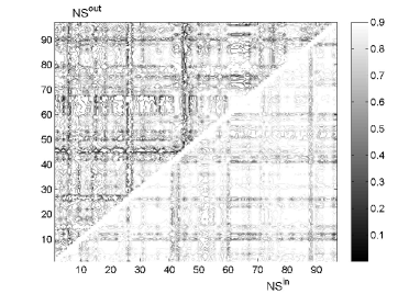
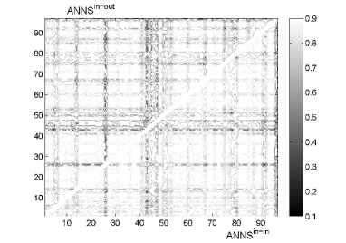
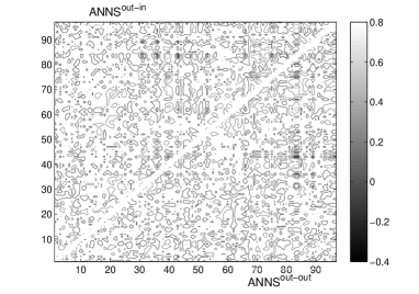
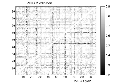
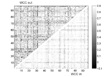
Figure 5 plots correlation patterns for some node statistics . Notice first that on average correlation coefficients are always positive for both $NS_{in}$ and $NS_{out}$, but those for $NS_{in}$ are larger than those for $NS_{out}$. This suggests that in general if a country exports (imports) more of a commodity, then it exports (imports) more of all other commodities. However, imports of different commodities are much more correlated than exports. This may be intuitively explained by the fact that (according to the HS classification) country imports may be related to inputs in the production process, which requires many different commodities. Instead, exports mainly regards the output process and they might therefore depend on the patterns of specialization of a country. The same behavior characterizes in- and out-types of clustering: countries that form intensive triangles where they import from two intensively-trading partners do so irrespectively of the commodity traded, but the correlation is higher than the corresponding pattern when now countries exports two intensively-trading partners.

An additional interesting insight comes from observing that in many cases darker stripes and lighter squares characterize the plots. Darker stripes are located typically on the edge between two adjacent 1-digit commodity classes, whereas squares with similar shades cover the entire 1-digit class. This means that in general correlation patterns mimic the HS classification, i.e. across-network correlations of a given statistics look similar when the commodity is similar according to the HS class —or abruptly change when one moves from a commodity class to another representing structurally different products and services. Interestingly, darker stripes often correspond to commodities that are less likely to be used as inputs then produced as outputs (manufactured product, typically retail oriented).

The fact that their statistics are more weakly correlated with those of other commodities hints to two different patterns as far as imports/exports and specialization patterns are concerned, and calls for further and deeper analyses. The fact that results partly mimic (or depend from) the classification scheme used indicate that it would be interesting to find classification-free grouping of commodities that are more data-driven. Data on cross-commodity correlations may be employed to address this issue, as we begin to study in the next section. The method we propose to study the problem is general, and represents a first step towards a systematic approach to the analysis of large multi-networks.

IV A framework for multi-network analysis

The above results show that the international trade network is not simply a superposition of independent commodity-specific layers. We found that significant correlations among layers make a comprehensive understanding of the structural properties of the whole system challenging. In particular, while single layers can certainly be studied independently using standard tools of network theory, a novel and more general framework of analysis is required in order to consistently take into account how different networks interact with each other to form the emerging aggregated network.

This problem is general, and not restricted to the particular system we are considering here. Besides a number of other economic and financial networks, that are virtually always systematically characterised by a superposition of product- or sector-specific relationships, other important examples include large social networks. Real social webs are believed to be the result of different means of interaction among actors, with ties of different types (friendship, coaffiliation, relatedness, etc.) cooperating to create a multiplex social network. Traditionally however, experimental constraints have limited the availability of real data, especially if reporting the different nature of social ties, to small networks. More recently, with the increasing availability of detailed large social network data, disentangling the different types of social relations is becoming possible also at a larger scale. Thus the type of problem we are facing here is likely to become of common interest in the near future for many research fields.

In what follows we make a first step in this direction by proposing a simple approach to characterise the mutual dependencies among layers in multi-networks, and their hierarchical organization. This approach is simple and general, and can therefore prove useful in the future for the analysis of other multi-networks emerging as the interaction of different sub-networks.

IV.1 Interdependency of layers

As a starting observation we note that, when studying a multi-network, the most detailed level of analysis focuses on the correlations between the presence, and the intensity in the weighted case, of single edges across different sub-networks. Inter-layer correlations between more aggregated properties (such as those we showed above between commodity-specific node degrees, node strengths, clustering coefficients, etc.) are ultimately due to these fundamental edge-level correlations. For this reason, one can perform a more detailed analysis by measuring inter-layer correlations according to any single observed interaction involving different layers. This analysis is possible at both weighted and unweighted levels for all the $C(C-1)/2$ pairs of layers, where $C$ is the total number of layers. As we show later on, the analysis of inter-layer correlations allows to define a hierarchy of layers. In the particular case of the trade system, this results in a taxonomy of commodities according to their roles in the world economy. We note that recent studies have already focused on the analysis of similarities among commodities, and on the associated reconstruction of a commodity space of goods, based on the observed patterns of revealed comparative advantage for countries Hidalgo et al. (2007); Hidalgo and Hausmann (2009), i.e. without specifically considering the structure of trade flows across countries. By constrast, the method that we use here allows to make use of more detailed information.

To be explicit, for each pair of layers $(c,c^{\prime})$, we consider the inter-layer correlation coefficient $\phi^{c,c^{\prime}}_{w}(t)$ between the corresponding edge weights:

$$\phi^{c,c^{\prime}}_{w}(t)\equiv\frac{\sum_{i\neq j}\left[w^{c}_{ij,t}-\overline{w^{c}_{t}}\right]\left[w^{c^{\prime}}_{ij,t}-\overline{w^{c^{\prime}}_{t}}\right]}{\sqrt{\sum_{i\neq j}\left[w^{c}_{ij,t}-\overline{w^{c}_{t}}\right]^{2}\sum_{i\neq j}\left[w^{c^{\prime}}_{ij,t}-\overline{w^{c^{\prime}}_{t}}\right]^{2}}},$$ (5)

where the subscript $w$ indicates that we are explicitly taking into account link weights, and $\overline{w^{c}_{t}}\equiv\sum_{i\neq j}w^{c}_{ij,t}/N(N-1)$ is the weight of links embedded in layer $c$, averaged over directed pairs of vertices. In our specific case study, $\overline{w^{c}_{t}}=1/N(N-1)$ is the traded volume of commodity $c$ averaged across all directed pairs of countries, which is idependent of $c$ due to the choice of the normalization. Similarly, if one focuses only on the topology and discards weights, it is possible to define the inter-layer correlation coefficient

$$\phi^{c,c^{\prime}}_{u}(t)\equiv\frac{\sum_{i\neq j}[a^{c}_{ij}(t)-\bar{a}^{c}(t)][a^{c^{\prime}}_{ij}(t)-\bar{a}^{c^{\prime}}(t)]}{\sqrt{\sum_{i\neq j}\left[a^{c}_{ij}(t)-\bar{a}^{c}(t)\right]^{2}\sum_{i\neq j}[a^{c^{\prime}}_{ij}(t)-\bar{a}^{c^{\prime}}(t)]^{2}}}$$ (6)

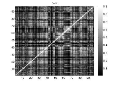
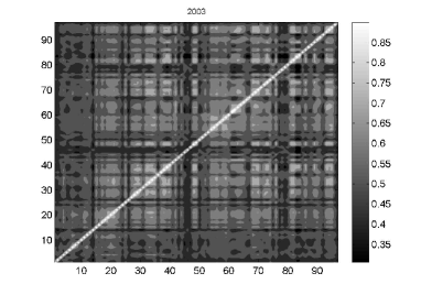
where $u$ stands for unweighted, and $\overline{a^{c}_{t}}\equiv\sum_{i\neq j}a^{c}_{ij,t}/N(N-1)$ is the fraction, measured across all directed pairs of vertices, of interactions involving layer $c$. Being Pearson’s correlation coefficients, $\phi^{c,c^{\prime}}_{w}(t)$ and $\phi^{c,c^{\prime}}_{u}(t)$ can take values in the range $[-1,+1]$, the two extrema representing complete anticorrelation and complete correlation respectively. Zero correlation is expected for statistically independent, non-interacting layers. Note that both quantities already take an overall size effect (total link weight and global link density respectively) into account. Therefore they allow comparisons across different years even if these overall properties are changing in time. For each year $t$ considered, eq.(5) gives rise to a $C\times C$ weighted inter-layer correlation matrix

$$\Phi_{w}(t)=\{\phi_{w}^{c,c^{\prime}}(t)\}$$ (7)

and eq.(6) gives rise to a $C\times C$ unweighted inter-layer correlation matrix

$$\Phi_{u}(t)=\{\phi_{u}^{c,c^{\prime}}(t)\}$$ (8)

both matrices being symmetric and with unit values along the diagonal.

In the case considered here, the above matrices quantify on an empirical basis how correlated are edges belonging to different layers. Large values of the correlation coefficient $\phi^{c,c^{\prime}}_{u}(t)$ signal that $c$ and $c^{\prime}$ play similar roles in the international trade system, as they are frequently traded together between pairs of countries (i.e. they often share the same importer and exporter country simultaneously). The quantity $\phi^{c,c^{\prime}}_{w}(t)$ measures the same effect, but also taking traded volumes into account. Although large correlations should in principle be observed more frequently for commodities of similar nature (“intrinsic” correlations) as they are expected to be both produced and consumed by similar sets of countries, they could be observed in more general cases as well (“revealed” correlations). Indeed, if intrinsically different commodities turn out to be highly correlated this can be interpreted as the result of favored trades of different goods between pairs of countries. For instance, in case of common geographic borders, trade agreements, or membership to the same free trade association or currency union, two countries $i$ and $j$ may prefer to exchange various types of commodities even if there are many potential alternative trade partners, either as importers or as exporters, for each commodity. Conversely, inter-layer correlations are decreased in presence of opposite trade preferences, i.e. by the tendency of pairs of countries to have specialized exchanges involving particular (sets of) commodities.

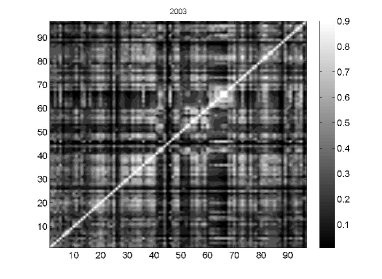
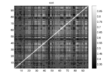
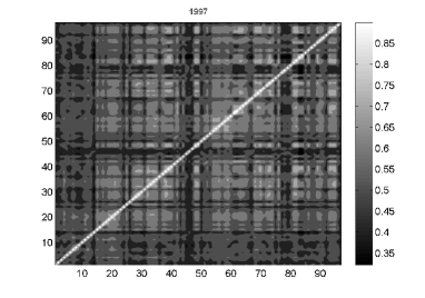
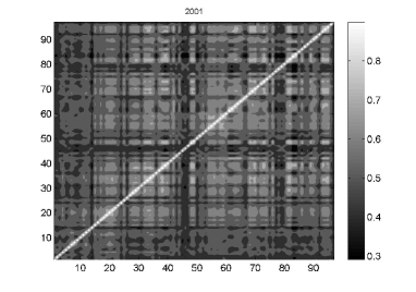
Plots of the matrices $\Phi_{w}(t)$ and $\Phi_{u}(t)$ are shown for various years in Figures 6 and 7 respectively. A first visual inspection suggests that in both cases the observed correlation structure is robust in time. However, as we show in section IV.3, it is possible to detect a small quantitative evolution of unweighted correlations, and to interpret it as the manifestation of an underlying dynamics of trade preferences determining “revealed’ correlations on top of “intrinsic” ones. Before describing that effect, in the following section we discuss the result of applying filtering procedures to inter-commodity correlation matrices.

IV.2 Hierarchies of layers

The correlation matrices defined in Eqs. (7) and (8) can be filtered exploiting a hierarchical procedure that has been introduced in financial analysis Mantegna (1999). Starting from the correlation coefficients $\phi^{c,c^{\prime}}_{w}(t)$ or $\phi^{c,c^{\prime}}_{u}(t)$ it is possible to define a weighted/unweighted inter-layer distance as follows:

$$d_{w/u}^{c,c^{\prime}}(t)\equiv\sqrt{\frac{1-\phi_{w/u}^{c,c^{\prime}}(t)}{2}}$$ (9)

Notice that here we are introducing a normalized variant of the transformation introduced in ref.Mantegna (1999). This has only an overall proportional effect on all distances, and does not change their ranking or their metric properties. We make this choice simply in order to have a maximum distance value $d_{w/u}^{c,c^{\prime}}=1$ when $c$ and $c^{\prime}$ are perfectly anticorrelated ($\phi_{w/u}^{c,c^{\prime}}=-1$), besides a minimum distance value $d_{w/u}^{c,c^{\prime}}=0$ when $c$ and $c^{\prime}$ are perfectly correlated ($\phi_{w/u}^{c,c^{\prime}}=1$). One should keep in mind that in case of no correlation ($\phi_{w/u}^{c,c^{\prime}}=0$) the above-defined distance equals $d_{w/u}^{c,c^{\prime}}=1/\sqrt{2}\approx 0.707$.

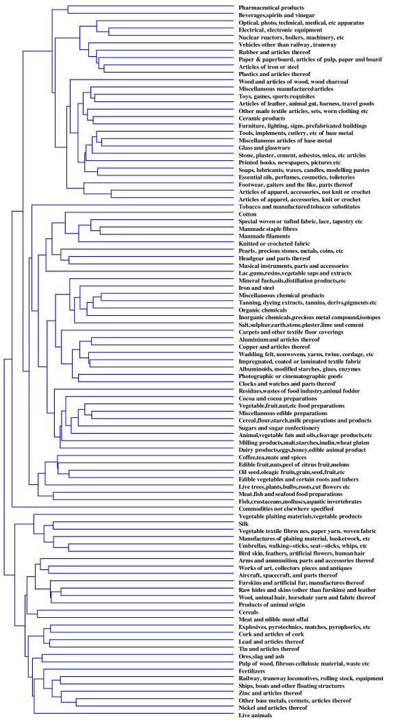
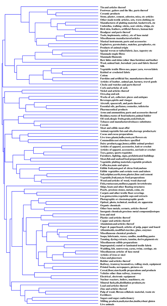
Once a distance matrix is given, one can filter it to obtain a dendrogram representing a taxonomy (hierarchical classification) of all layers. In such a representation, the $C$ layers are the leaves of the taxonomic tree. Closer (strongly correlated) layers meet at a branching point closer to the leaf level, while more distant (weakly correlated) layers meet at a more distant branching point. All layers eventually merge at a single root level. If the tree is cut at some level, it splits in disconnected branches of similar (with respect to the cut level chosen) layers. The hierarchical nature of the classification is manifest in the nestedness of the dendrogram. A detailed description of possible procedures to obtain the taxonomic tree can be found in Ref. Mantegna (1999).

In Figure 8 we show the dendrogram of commodities obtained applying the Complete Linkage Clustering Algorithm to the unweighted inter-layer distances $d^{c,c^{\prime}}_{u}(t)$ measured in year $t=2003$. Similarly, in Figure 9 we show we dendrogram obtained applying the same algorithm to the weighted inter-layer distances $d^{c,c^{\prime}}_{w}(t)$ measured in the same year. In both dendrograms one can observe that while in some cases similar commodities (such as the textiles and leather sectors) are grouped together, in other cases a-priori unrelated goods are found to belong to the same clusters. This confirms that, on top of an intrinsic structure of inter-commodity correlations, “revealed” effects are taking place. While it is not possible to disentangle these two contributions on the basis of observed trade interactions alone, in the next section we describe how we expect the two types of correlation to undergo different, empirically observable, dynamical patterns.

IV.3 Evolution of inter-layer correlations and distances

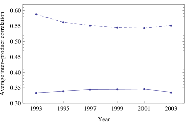
The previous results highlight that inter-commodity correlations are a combination of “revealed” contributions, arising as commodity-independent results of preferences in trade partnerships between countries, and intrinsic contributions, due to inherent commodity similarities. We now describe a way to assess whether “revealed” correlations develop in time on top of intrinsic correlations. While the classification of trade commodities is static (i.e. commodities do not become more or less similar as time proceeds), the correlations among them may vary in time. This implies that while intrinsic correlations are expected to remain essentially stable in time as they merely reflect the internal similarities already present in the commodity structure, revealed correlation could in principle evolve in response of some dynamics of trade preferences. Therefore we expect the time evolution of inter-layer correlations and distances to reflect underlying changes in trade preferences. Moreover, we expect trade preferences to affect unweighted correlations more strongly than weighted correlations, as they will primarily determine the presence or absence of multiple types of traded commodities, while volumes will be also affected by the specific sizes of production and demand.

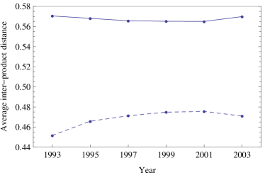
We can study this effect in an aggregated fashion by defining the average weighted/unweighted inter-layer correlation

$$\bar{\phi}_{w/u}(t)\equiv\frac{\sum_{c\neq c^{\prime}}\phi_{w/u}^{c,c^{\prime}}(t)}{C(C-1)}=\frac{2\sum_{c<c^{\prime}}\phi_{w/u}^{c,c^{\prime}}(t)}{C(C-1)}$$ (10)

or, conversely, the average weighted/unweighted inter-layer distance

$$\bar{d}_{w/u}(t)\equiv\frac{\sum_{c\neq c^{\prime}}d_{w/u}^{c,c^{\prime}}(t)}{C(C-1)}=\frac{2\sum_{c<c^{\prime}}d_{w/u}^{c,c^{\prime}}(t)}{C(C-1)}$$ (11)

and following their evolution in time. Of course correlation and distance measures are linked by (9). Therefore, strictly speaking, the only value added in studying them together is because they offer two complementary interpretations of the same phenomenon.

The results are shown in Figure 10. Note that the averages are performed over all $C(C-1)/2$ commodity pairs. If all commodities were uncorrelated one would have $\bar{\phi}_{w/u}=0$ and $\bar{d}_{w/u}=1/\sqrt{2}$. The trends indicate that indeed a dynamics of “revealed” correlations is present. From year 1993 to year 2001, the average unweighted inter-layer correlation $\bar{\phi}_{u}(t)$ has been decreasing steadily over time, and correspondingly the average unweighted inter-layer distance $\bar{d}_{u}(t)$ has been increasing. This means that, on average, the roles played by different commodities in the international trade system have become more and more dissimilar. The corresponding weighted quantities display much smaller variations. We interpret these results as the enhancement of trade specialization during the corresponding period, with pairs of countries developing more and more commodity-intensive trade relationships characterized by a decreasing variety of goods. As expected, this effect is more pronounced for unweighted measures than for weighted measures, as the latter also aggregate economy-specific size effects. However, from year 2001 to year 2003 an inversion in the trend is observed. Whether this is due to an actual inversion of trade preferences is an important open point that requires further clarification.

V Concluding remarks

In this paper we have begun to study the statistical properties of the multi-network of international trade, and their evolution over time. We have employed data on commodity-specific trade flows to build a sequence of graphs where any two nodes (countries) are connected by many weighted directed edges, each one representing the flow of export from the origin to the target country for a given specific commodity class.

We have characterized the topological properties of all commodity-specific networks and compared them to those of the aggregate-trade network. Furthermore, we have studied both within- and across-network correlation patterns between topological statistics, and tracked the time evolution of the largest connected components in the commodity-specific networks. Finally, we have proposed a general approach to study multi-networks using detailed edge-level correlations among layers. This method allows to resolve the hierarchical organisation of inter-layer dependencies. When applied to the trade network, it allows to define correlation-based inter-layer distances that are helpful in taxonomizing commodities not only with respect to the inherent similarity between commodities, but also with respect to the actual revealed trade patterns.

The preliminary nature of the present work opens the way to many possible extensions. For instance, one might consider to employ filtering techniques such as those use in Ref. Serrano et al. (2007) to extract in a multi-network perspective a backbone of most-relevant trade-relationships between countries that take into account, beside their geographical position and relative size, also a third dimension defined by the type of commodities mostly traded. Similarly, community detection techniques like the ones used in Ref. (Tzekina et al., 2008) may be extended to multi-network setups in order to single out tightly-interconnected groups of countries, and possibly compare them to the implications of international-trade models. Finally, the robustness of statistical properties of the ITMNs might be checked against alternative weighting schemes that, for example, control for country size and geographical distance, much in the spirit of gravity models in international trade literature (Overman et al., 2003; Fratianni, 2009).

Table 1: Harmonized System 1996 Classification of Commodities

Code	Description
01	Live animals
02	Meat and edible meat offal
03	Fish, crustaceans & aquatic invertebrates
04	Dairy produce; birds eggs; honey and other edible animal products
05	Other products of animal origin
06	Live trees, plants; bulbs, roots; cut flowers & ornamental foliage te & spices
07	Edible vegetables & certain roots & Tubers
08	Edible fruit & nuts; citrus fruit or melon peel
09	Coffee, tea, mate & spices
10	Cereals
11	Milling products; malt; starch; inulin; wheat gluten
12	Oil seeds & oleaginous fruits; miscellaneous grains, seeds & fruit; industrial or medicinal plants; straw & fodder
13	Lac; gums, resins & other vegetable sap & extracts
14	Vegetable plaiting materials & other vegetable products
15	Animal,vegetable fats and oils, cleavage products, etc
16	Edible preparations of meat, fish, crustaceans, molluscs or other aquatic invertebrates
17	Sugars and sugar confectionary
18	Cocoa and cocoa preparations
19	Preparations of cereals, flour, starch or milk; bakers wares
20	Preparations of vegetables, fruit, nuts or other plant parts
21	Miscellaneous edible preparations
22	Beverages, spirits and vinegar
23	Food industry residues & waste; prepared animal feed
24	Tobacco and manufactured tobacco substitutes
25	Salt; sulfur; earth & stone; lime & cement plaster
26	Ores, slag and ash
27	Mineral fuels, mineral oils & products of their distillation; bitumin substances; mineral wax
28	Inorganic chemicals; organic or inorganic compounds of precious metals, of rare-earth metals, of radioactive elements or of isotopes
29	Organic chemicals
30	Pharmaceutical products
31	Fertilizers
32	Tanning or dyeing extracts; tannins & derivatives; dyes, pigments & coloring matter; paint & varnish; putty & other mastics; inks
33	Essential oils and resinoids; perfumery, cosmetic or toilet preparations
34	Soap; waxes; polish; candles; modelling pastes; dental preparations with basis of plaster
35	Albuminoidal substances; modified starch; glues; enzymes
36	Explosives; pyrotechnic products; matches; pyrophoric alloys; certain combustible preparations
37	Photographic or cinematographic goods
38	Miscellaneous chemical products
39	Plastics and articles thereof.
40	Rubber and articles thereof.
41	Raw hides and skins (other than furskins) and leather
42	Leather articles; saddlery and harness; travel goods, handbags & similar; articles of animal gut [not silkworm gut]
43	Furskins and artificial fur; manufactures thereof
44	Wood and articles of wood; wood charcoal
45	Cork and articles of cork
46	Manufactures of straw, esparto or other plaiting materials; basketware & wickerwork
47	Pulp of wood or of other fibrous cellulosic material; waste & scrap of paper & paperboard
48	Paper & paperboard & articles thereof; paper pulp articles ts and plans
49	Printed books, newspapers, pictures and other products of printing industry; manuscripts, typescrip
50	Silk, including yarns and woven fabric thereof
51	Wool & animal hair, including yarn & woven fabric
52	Cotton, including yarn and woven fabric thereof
53	Other vegetable textile fibers; paper yarn and woven fabrics of paper yarn
54	Manmade filaments, including yarns & woven fabrics
55	Manmade staple fibres, including yarns & woven fabrics
56	Wadding, felt and nonwovens; special yarns; twine, cordage, ropes and cables and articles thereof
57	Carpets and other textile floor coverings
58	Special woven fabrics; tufted textile fabrics; lace; tapestries; trimmings; embroidery
59	Impregnated, coated, covered or laminated textile fabrics; textile articles for industrial use
60	Knitted or crocheted fabrics
61	Apparel articles and accessories, knitted or crocheted
62	Apparel articles and accessories, not knitted or crocheted
63	Other textile articles; needlecraft sets; worn clothing and worn textile articles; rags
64	Footwear, gaiters and the like and parts thereof
65	Headgear and parts thereof
66	Umbrellas, walking-sticks, seat-sticks, riding-crops, whips, and parts thereof
67	Prepared feathers, down and articles thereof; artificial flowers; articles of human hair
68	Articles of stone, plaster, cement, asbestos, mica or similar materials
69	Ceramic products
70	Glass and glassware
71	Pearls, precious stones, metals, coins, etc
72	Iron and steel
73	Articles of iron or steel
74	Copper and articles thereof
75	Nickel and articles thereof
76	Aluminum and articles thereof
78	Lead and articles thereof
79	Zinc and articles thereof
80	Tin and articles thereof
81	Other base metals; cermets; articles thereof
82	Tools, implements, cutlery, spoons & forks of base metal & parts thereof
83	Miscellaneous articles of base metal
84	Nuclear reactors, boilers, machinery and mechanical appliances; parts thereof
85	Electric machinery, equipment and parts; sound equipment; television equipment
86	Railway or tramway. Locomotives, rolling stock, track fixtures and parts thereof; mechanical & electro-mechanical traffic signal equipment
87	Vehicles, (not railway, tramway, rolling stock); parts and accessories
88	Aircraft, spacecraft, and parts thereof
89	Ships, boats and floating stuctures
90	Optical, photographic, cinematographic, measuring, checking, precision, medical or surgical instruments/apparatus; parts & accessories
91	Clocks and watches and parts thereof
92	Musical instruments; parts and accessories thereof
93	Arms and ammunition, parts and accessories thereof
94	Furniture; bedding, mattresses, cushions etc; other lamps & light fitting, illuminated signs and nameplates, prefabricated buildings
95	Toys, games & sports equipment; parts & accessories
96	Miscellaneous manufactured articles
97	Works of art, collectors pieces and antiques
99	Commodities not elsewhere specified

HS Code	Commodity	Value (USD)	Value per Link (USD)	$\%$ of Aggregate Trade
84	Nuclear reactors, boilers, machinery and mechanical appliances; parts thereof	$5.67\times 10^{11}$	$6.17\times 10^{7}$	11.37%
85	Electric machinery, equipment and parts; sound equipment; television equipment	$5.58\times 10^{11}$	$6.37\times 10^{7}$	11.18%
27	Mineral fuels, mineral oils & products of their distillation; bitumin substances; mineral wax	$4.45\times 10^{11}$	$9.91\times 10^{7}$	8.92%
87	Vehicles, (not railway, tramway, rolling stock); parts and accessories	$3.09\times 10^{11}$	$4.76\times 10^{7}$	6.19%
90	Optical, photographic, cinematographic, measuring, checking, precision, medical or surgical instruments/apparatus; parts & accessories	$1.78\times 10^{11}$	$2.48\times 10^{7}$	3.58%
39	Plastics and articles thereof.	$1.71\times 10^{11}$	$2.33\times 10^{7}$	3.44%
29	Organic chemicals	$1.67\times 10^{11}$	$3.29\times 10^{7}$	3.35%
30	Pharmaceutical products	$1.4\times 10^{11}$	$2.59\times 10^{7}$	2.81%
72	Iron and steel	$1.35\times 10^{11}$	$2.77\times 10^{7}$	2.70%
71	Pearls, precious stones, metals, coins, etc	$1.01\times 10^{11}$	$2.41\times 10^{7}$	2.02%
10	Cereals	$3.63\times 10^{10}$	$1.28\times 10^{7}$	0.73%
52	Cotton, including yarn and woven fabric thereof	$3.29\times 10^{10}$	$6.96\times 10^{6}$	0.66%
9	Coffee, tea, mate & spices	$1.28\times 10^{10}$	$2.56\times 10^{6}$	0.26%
93	Arms and ammunition, parts and accessories thereof	$4.31\times 10^{9}$	$2.46\times 10^{6}$	0.09%
ALL	Aggregate	$4.99\times 10^{12}$	$3.54\times 10^{8}$	100.00%

Table 2: The 14 most relevant commodity classes in year 2003 in terms of total-trade value (USD), trade value per link (USD), and share of world aggregate trade.

HS Code	Commodity	$w_{ij}$	Density	$NS_{in}/ND_{in}$	$NS_{out}/ND_{out}$	$WCC_{all}$
9	Coffee	282%	27%	192%	177%	176%
10	Cereals	497%	15%	540%	201%	218%
27	Min. Fuels	314%	24%	255%	282%	190%
29	Org. Chem.	277%	28%	218%	133%	176%
30	Pharmaceutical	260%	29%	248%	111%	151%
39	Plastics	192%	40%	173%	107%	119%
52	Cotton	298%	26%	227%	162%	220%
71	Prec. Metals	337%	23%	192%	206%	151%
72	Iron	290%	26%	243%	145%	182%
84	Nuclear Machin.	153%	50%	140%	101%	109%
85	Electric Machin.	161%	48%	139%	102%	109%
87	Vehicles	217%	35%	201%	106%	115%
90	Optical Instr.	196%	39%	153%	104%	112%
93	Arms	804%	10%	576%	350%	375%

Table 3: Density and node-average of topological properties of commodity-specific networks vs. aggregate trade network for the 14 most relevant commodity classes in year 2003. Percentages refer to the ratio of the statistic value in the commodity-specific network to aggregate network. Values larger (smaller) than 100% mean that average of commodity-specific networks is larger (smaller) than its counterpart in the aggregate network.

		Clustering Pattern
HS Code	Commodity	Cycle	Middleman	In	Out
09	Coffee and spices	2.77%	18.81%	34.92%	43.50%
10	Cereals	2.19%	14.86%	57.93%	25.02%
27	Mineral fuels	3.13%	20.66%	39.18%	37.03%
29	Organic chemicals	8.94%	11.06%	49.47%	30.53%
30	Pharmaceutical products	4.93%	6.13%	64.79%	24.15%
39	Plastics	7.73%	10.52%	51.54%	30.21%
52	Cotton	7.71%	12.94%	44.13%	35.22%
71	Precious metals	14.00%	15.84%	17.72%	52.44%
72	Iron and steel	7.13%	15.40%	45.28%	32.20%
84	Nuclear machinery	7.77%	9.46%	51.88%	30.89%
85	Electric machinery	9.27%	10.33%	48.15%	32.26%
87	Vehicles	5.49%	7.45%	57.48%	29.58%
90	Optical instruments	9.10%	10.63%	48.39%	31.88%
93	Arms	6.69%	13.74%	54.68%	24.90%
All	Aggregate	20.21%	20.69%	22.46%	36.64%

Table 4: Relative frequency of the occurrence of clustering patterns in the aggregate and commodity-specific networks.

Area	N	1993	1995	1997	1999	2001	2003
Core EU	8	63%	100%	100%	100%	100%	100%
Periphery EU	10	90%	100%	100%	100%	100%	100%
Eastern Europe	15	20%	53%	93%	100%	93%	93%
North and Central America	22	59%	73%	91%	95%	91%	82%
South America	12	58%	92%	83%	100%	100%	83%
South and East Asia	20	65%	55%	65%	70%	75%	80%
Central Asia	8	13%	25%	50%	50%	38%	63%
North Africa and Middle East	18	39%	56%	56%	61%	78%	78%
Sub-Saharan Africa	40	18%	58%	65%	70%	70%	53%
Oceania	9	33%	33%	33%	33%	44%	56%
World	162	41%	63%	72%	77%	79%	74%

Table 5: Size of the largest connected component as a percentage of total network size across geographical macro-areas and time in the aggregate (all-commodity) trade network. Here two nodes are said to be connected if they are linked by a bilateral edge (both import and export relationship).

HS Code	Commodity	All	Largest 10%	Largest 5%	Largest 1%
09	Coffee and spices	119	46	23	4
10	Cereals	107	25	15	3
27	Mineral fuels	117	45	28	9
29	Organic chemicals	117	41	29	11
30	Pharmaceutical products	117	40	23	10
39	Plastics	120	57	40	19
52	Cotton	116	45	29	12
71	Precious metals	114	42	27	11
72	Iron and steel	119	45	33	14
84	Nuclear machinery	120	45	39	21
85	Electric machinery	120	48	39	19
87	Vehicles	120	46	34	14
90	Optical instruments	120	48	33	14
93	Arms	80	23	17	5
All	Aggregate	162	81	58	28

Table 6: Size of the largest connected component in aggregate and commodity-specific networks in year 2003. All: A binary link is in place if the associated link weight is larger than zero; Largest x%: A binary link is in place if the associated link weight belongs to the set of x% largest link-weights. Here we assume that two nodes are connected if either an inward or an outward link is in place.

HS Code	Commodity	Size of LCC	Countries in the LCC
09	Coffee and spices	4	Canada; Germany; Italy; USA
10	Cereals	3	Canada; Germany; USA
27	Mineral fuels	9	Canada; China; Germany; Indonesia; Korea; Malaysia; Singapore; UK; USA
29	Organic chemicals	11	Canada; China; France; Germany; Italy; Japan; Korea; Netherlands; Switzerland; UK; USA
30	Pharmaceutical products	10	Canada; France; Germany; Italy; Japan; Netherlands; Spain; Switzerland; UK; USA
39	Plastics	19	Austria; Canada; China; France; Germany; Hong Kong; Italy; Japan; Korea; Malaysia; Mexico; Netherlands; Poland; Singapore; Spain; Switzerland; Thailand; UK; USA
52	Cotton	12	China; France; Germany; Hong Kong; Italy; Japan; Korea; Mexico; Pakistan; Spain; Turkey; USA
71	Precious metals	11	Australia; Belgium-Luxembourg; Canada; Hong Kong; India; Israel; Italy; Korea; Switzerland; UK; USA
72	Iron and steel	14	Austria; Canada; China; France; Germany; Italy; Japan; Korea Mexico; Netherlands; Russia; Spain; UK; USA
84	Nuclear machinery	21	Austria; Brazil; Canada; China; France; Germany; Ireland; Italy; Japan; Korea; Malaysia; Mexico; Netherlands; Philippines; Poland; Singapore; Spain; Sweden; Thailand; UK; USA
85	Electric machinery	19	Austria; Canada; China; France; Germany; Hong Kong; Hungary; Italy; Japan; Korea; Malaysia; Mexico; Netherlands; Philippines; Singapore; Switzerland; Thailand; UK; USA
87	Vehicles	14	Canada; China; France; Germany; Hungary; Italy; Japan; Mexico; Netherlands; Poland; Spain; Sweden; UK; USA
90	Optical instruments	14	Canada; China; France; Germany; Hong Kong; Ireland; Italy; Japan; Mexico; Netherlands; Singapore; Switzerland; UK; USA
93	Arms	5	Canada; Italy; Japan; Spain; USA
All	Aggregate	28	Australia; Austria; Brazil; Canada; China; Denmark; France Germany; Hong Kong; Hungary; Ireland; Italy; Japan; Korea; Malaysia; Mexico; Netherlands; Philippines; Poland; Russia Singapore; Spain; Sweden; Switzerland; Thailand; Turkey UK; USA

Table 7: Size and composition of the largest-connected component (LCC) in aggregate and commodity-specific networks in year 2003. A binary link is in place if the associated link weight belongs to the set of 1% largest link-weights. Here we assume that two nodes are connected if either an inward or an outward link is in place.

	$NS_{in}$			$NS_{out}$			$NS_{tot}$
Commodity	1st	2nd	3rd	1st	2nd	3rd	1st	2nd	3rd
Coffee & spices	USA	Germany	Japan	Brazil	Colombia	Indonesia	USA	Germany	Brazil
Cereals	Japan	Mexico	Korea	USA	France	Argentina	USA	Japan	France
Mineral fuels	USA	Japan	China	Russia	Saudi Arabia	Norway	USA	Russia	China
Organic chemicals	USA	China	Germany	USA	Ireland	Germany	USA	Germany	France
Pharmaceutical products	USA	Germany	UK	USA	Germany	France	USA	Germany	UK
Plastics	China	USA	Germany	Germany	USA	Japan	Germany	USA	China
Cotton	Hong Kong	China	USA	China	USA	Italy	China	USA	Hong Kong
Precious metals	USA	Hong Kong	UK	Switzerland	India	USA	USA	India	Switzerland
Iron & steel	China	USA	Italy	Japan	Germany	Russia	Germany	China	Japan
Nuclear machinery	USA	UK	Germany	Germany	USA	China	USA	Germany	China
Electric machinery	Germany	USA	UK	USA	China	Germany	USA	Germany	China
Vehicles	Germany	USA	UK	Germany	Japan	France	Germany	Japan	UK
Optical instruments	USA	Germany	UK	USA	Germany	Japan	USA	Germany	Japan
Arms	USA	UK	Korea	USA	Germany	Italy	USA	UK	Germany
Aggregate	USA	Germany	UK	USA	Germany	China	USA	Germany	China

Table 8: Country rankings in 2003. Top 3 position according to node strength statistics.

	$NS_{in-in}$			$NS_{out-in}$
Commodity	1st	2nd	3rd	1st	2nd	3rd
Coffee & spices	Cambodia	Dominica	Guyana	St. Kitts & Nevis	Eq. Guinea	Vanuatu
Cereals	Sao Tome	Papua New Guinea	Samoa	Mongolia	Nepal	Morocco
Mineral fuels	C. African Rep	Samoa	Grenada	Guinea Bissau	Mauritania	DemRepCongo
Organic chemicals	C. African Rep	Gambia	St. Vincent	Vanuatu	Guyana	St. Vincent
Pharmaceutical products	C. African Rep	Samoa	Maldives	Bahamas	Nepal	Kyrgyzstan
Plastics	C. African Rep	Samoa	Maldives	Comoros	Eq. Guinea	Mongolia
Cotton	St. Lucia	Belize	Mongolia	Mongolia	Laos	Malawi
Precious metals	Gabon	St. Kitts & Nevis	Gambia	Cape Verde	St.Lucia	Eq. Guinea
Iron & steel	Samoa	Nepal	Grenada	Mongolia	Papua New Guinea	Sao Tome
Nuclear machinery	Sao Tome	Samoa	Brunei Darussalam	Eq. Guinea	Rwanda	C. African Rep
Electric machinery	C. African Rep	Samoa	Sao Tome	Kiribati	Djibouti	Mongolia
Vehicles	St. Kitts & Nevis	Sao Tome	Dominica	Suriname	Sao Tome	Cape Verde
Optical instruments	Samoa	C. African Rep	Gambia	St. Vincent	Haiti	Cape Verde
Arms	St. Kitts & Nevis	Papua New Guinea	Dominica	Ecuador	Haiti	Albania
Aggregate	Sao Tome	Samoa	Maldives	Tonga	St.Lucia	Kiribati
	$NS_{out-out}$			$NS_{in-out}$
Commodity	1st	2nd	3rd	1st	2nd	3rd
Coffee & spices	Bhutan	St. Kitts & Nevis	Chad	Guyana	ElSalvador	Ecuador
Cereals	Armenia	Bhutan	Jamaica	C. African Rep	Samoa	Guyana
Mineral fuels	Mongolia	Tajikistan	Kyrgyzstan	Hong Kong	Gabon	Rwanda
Organic chemicals	St. Vincent	Tajikistan	Eq. Guinea	Gambia	C. African Rep	Cambodia
Pharmaceutical products	Bahamas	Suriname	Nepal	C. African Rep	Samoa	Gambia
Plastics	St. Kitts & Nevis	Comoros	Grenada	C. African Rep	Samoa	Maldives
Cotton	Mongolia	Bahamas	Gambia	St.Lucia	Dominica	Belize
Precious metals	Kiribati	Uganda	Cape Verde	Guyana	Samoa	Malawi
Iron & steel	Sao Tome	Madagascar	Sierra Leone	Mongolia	Brunei Darussalam	Nepal
Nuclear machinery	Eq. Guinea	Cape Verde	St. Kitts & Nevis	Sao Tome	Samoa	St. Kitts & Nevis
Electric machinery	Kiribati	Tajikistan	Mongolia	Sao Tome	Samoa	Belize
Vehicles	Suriname	SolomonIsds	Sao Tome	Sao Tome	St. Kitts & Nevis	Dominica
Optical instruments	St. Vincent	Haiti	Cape Verde	C. African Rep	Samoa	Gambia
Arms	Ecuador	Haiti	Albania	St. Kitts & Nevis	Papua New Guinea	Dominica
Aggregate	Tonga	St.Lucia	Bhutan	Sao Tome	Samoa	Maldives

Table 9: Country rankings in 2003. Top 3 position according to node ANNS statistics.

	$WCC_{all}$			$WCENTR$
Commodity	1st	2nd	3rd	1st	2nd	3rd
Coffee & spices	Colombia	Brazil	Vietnam	Brazil	Colombia	Indonesia
Cereals	Algeria	Papua New Guinea	Tunisia	USA	Canada	Thailand
Mineral fuels	Eq. Guinea	Libya	Angola	Russia	Saudi Arabia	Norway
Organic chemicals	Eq. Guinea	USA	Japan	Ireland	USA	Germany
Pharmaceutical products	USA	Germany	France	USA	Germany	France
Plastics	Germany	USA	China	Germany	USA	Netherlands
Cotton	Uzbekistan	China	Italy	China	USA	Pakistan
Precious metals	Israel	Uzbekistan	Angola	Switzerland	India	UK
Iron & steel	Germany	Italy	China	Germany	France	Japan
Nuclear machinery	China	USA	Germany	China	Japan	USA
Electric machinery	China	USA	Germany	USA	Japan	China
Vehicles	Germany	Japan	USA	Germany	Japan	UK
Optical instruments	USA	China	Japan	USA	China	Japan
Arms	Saudi Arabia	Norway	USA	USA	Germany	Italy
Aggregate	USA	Germany	China	USA	China	Germany

Table 10: Country rankings in 2003. Top 3 position according to node overall clustering and centrality statistics.

		Correlation Coefficient
		$NS_{in}$	$NS_{out}$	$ANNS_{tot}$	$ANNS_{in-in}$	$ANNS_{in-out}$	$ANNS_{out-in}$	$ANNS_{out-out}$	$WCC_{all}$	$WCC_{in}$	$WCC_{out}$	$WCENTR$
HS Code	Commodity	$ND_{in}$	$ND_{out}$	$NS_{tot}$	$NS_{in}$	$NS_{in}$	$NS_{out}$	$NS_{out}$	$NS_{tot}$	$NS_{in}$	$NS_{out}$	$NS_{tot}$
09	Coffee & spices	0.5916	0.6311	-0.3511	-0.0922	-0.0527	-0.2666	-0.0777	0.6462	0.7485	0.7283	0.6247
10	Cereals	0.4663	0.6454	-0.1151	0.1704	0.0592	-0.0119	-0.0522	0.3130	0.7328	0.5663	0.7957
27	Mineral fuels	0.6615	0.4937	-0.1746	-0.0474	0.1631	-0.0208	0.0121	0.3629	0.8605	0.5195	0.7295
29	Organic chemicals	0.5256	0.6242	-0.2428	-0.0918	-0.0808	-0.1721	-0.1583	0.7810	0.8484	0.7227	0.9116
30	Pharmaceutical products	0.4642	0.5876	-0.2123	-0.0053	-0.0266	-0.1489	-0.1489	0.9148	0.7677	0.9681	0.9702
39	Plastics	0.5828	0.5376	-0.3610	-0.0452	-0.0672	-0.2942	-0.2990	0.9148	0.7721	0.9600	0.9667
52	Cotton	0.6226	0.6455	-0.3280	-0.0921	-0.1310	-0.1845	-0.1849	0.5967	0.7668	0.5322	0.8843
71	Precious metals	0.6263	0.6775	-0.3437	-0.1531	-0.1328	-0.2790	-0.3125	0.6860	0.7624	0.6691	0.9097
72	Iron and steel	0.5478	0.7140	-0.3694	-0.0323	-0.0139	-0.2158	-0.2081	0.8386	0.8798	0.7900	0.8559
84	Nuclear machinery	0.6630	0.5618	-0.5377	-0.0676	-0.0948	-0.4667	-0.4511	0.9323	0.7680	0.9782	0.9567
85	Electric machinery	0.6431	0.5916	-0.5069	-0.1002	-0.1122	-0.4753	-0.4526	0.9327	0.7927	0.9752	0.9494
87	Vehicles	0.5938	0.5165	-0.3498	-0.0150	-0.0635	-0.2659	-0.2440	0.9171	0.7435	0.9612	0.9746
90	Optical instruments	0.6134	0.4819	-0.3634	-0.1299	-0.1400	-0.3173	-0.2868	0.9105	0.7414	0.9588	0.9564
93	Arms	0.5948	0.6956	-0.1215	-0.0422	-0.0476	-0.0553	-0.0659	0.5374	0.7078	0.4825	0.8358
All	Aggregate	0.4453	0.4620	-0.4017	-0.1437	-0.1412	-0.4348	-0.4377	0.9669	0.9494	0.9760	0.9779

Table 11: Correlation coefficients between topological statistics within each commodity-network in year 2003.

Figure 1: Scatter plot of total-trade value vs. trade value per link of all 96 commodity classes in year 2003. Natural logarithms on both axes.

Figure 2: Node in-strength per inward link vs node out-strength per outward link of all 96 commodity classes in year 2003.

Figure 3: Average vs. standard deviation of link-weight distribution in 2003.

Figure 4: Distributions of positive link weights in 2003. 10: Cereals; 27: Mineral Fuels; 72: Iron and steel; 93: Arms. Solid line: Normal fit.

Figure 5: Correlation coefficients of topological statistics across networks. Axes represent HS classification codes. When convenient, each plot contains the correlation patterns for two statistics, one in the upper-left triangle and another in the bottom-right triangle.

Figure 6: Plots of weighted inter-layer correlation matrices $\Phi_{w}(t)$ for years $t=1993,1995,1997,1999,2001,2003$.

Figure 7: Plots of unweighted inter-layer correlation matrices $\Phi_{u}(t)$ for years $t=1993,1995,1997,1999,2001,2003$.

Figure 8: Dendrogram of commodities obtained applying the Complete Linkage Clustering Algorithm to the unweighted inter-layer distances $d^{c,c^{\prime}}_{u}(t)$ measured in year $t=2003$.

Figure 9: Dendrogram of commodities obtained applying the Complete Linkage Clustering Algorithm to the weighted inter-layer distances $d^{c,c^{\prime}}_{w}(t)$ measured in year $t=2003$.

Figure 10: Left: evolution of average weighted inter-layer correlation $\bar{\phi}_{w}(t)$ (solid) and average unweighted inter-layer correlation $\bar{\phi}_{u}(t)$ (dashed) from year $t=1993$ to year $t=2003$. Right: evolution of average weighted inter-layer distance $\bar{d}_{w}(t)$ (solid) and average unweighted inter-layer distance $\bar{d}_{u}(t)$ (dashed) from year $t=1993$ to year $t=2003$.