How Small Are Building Blocks of Complex Networks
Abstract
Network motifs are small building blocks of complex networks. Statistically significant motifs often perform network-specific functions. However, the precise nature of the connection between motifs and the global structure and function of networks remains elusive. Here we show that the global structure of some real networks is statistically determined by the probability of connections within motifs of size at most , once this probability accounts for node degrees. The connectivity profiles of node triples in these networks capture all their local and global properties. This finding impacts methods relying on motif statistical significance, and enriches our understanding of the elementary forces that shape the structure of complex networks.
I Introduction
A promising direction in the study of the structure and function of complex networks is to identify their building blocks, or motifs Milo et al. (2002); Alon (2007, 2006), which are small subgraphs in a real network. A great deal of research—in particular, research on gene regulatory networks—shows that specific motifs perform specific functions, such as speeding up response times of regulatory networks Rosenfeld et al. (2002); Mangana et al. (2006). However, motifs have also raised many questions Knabe et al. (2008a); Ingram et al. (2006); Cordero and Hogeweg (2006); Kuo et al. (2006); Mazurie et al. (2005); Sakata et al. (2005); Vázquez et al. (2004); Artzy-Randrup et al. (2004), including continuing debates on whether and how motif statistical profiles are related to the global structure, function, and evolution of certain networks. Our recent work Mahadevan et al. (2006a) introduces -series, see Section II.
The -series, with analogy to the Taylor or Fourier series, is a systematic and complete basis for characterizing network structure. The -series subsumes many known motif- and degree-based statistical characteristics of complex networks. While motifs are subgraphs whose nodes can have any degree in a given real network, the -series preserves the information about these degrees. For example, the zero-th element of the -series, the -“distribution,” is the average degree in a given network. The first element, the -distribution, is the network’s degree distribution, or the number of nodes—subgraphs of size —of degree . The second element, the -distribution, is the joint degree distribution, the number of subgraphs of size —links—involving nodes of degrees and . The -distribution thus defines -node degree correlations. For , the subgraphs are triangles and wedges, composed of nodes of degrees , , and , which defines clustering. Generalizing, the -distribution is the numbers of different subgraphs of size involving nodes of degrees .
The -series is systematic and complete because it is inclusive and converging. Inclusiveness results from the fact that the -distribution contains the same information about the network as the -distribution, plus some additional information. That is, by increasing , we provide strictly more detail about the network structure, which is not the case with a motif-based series. Node degrees are necessary to make the series inclusive and thus systematic, see Section V. As increases toward the network size, we fully specify the entire network structure, which explains the second convergence property of -series—it converges to the given network in the limit of large .
Does this convergence happen only at equal to the network size, or much sooner, at smaller ? In other words, how much local information, i.e., information about concentrations of degree-labeled subgraphs of what size, is needed to fully capture global network structure?
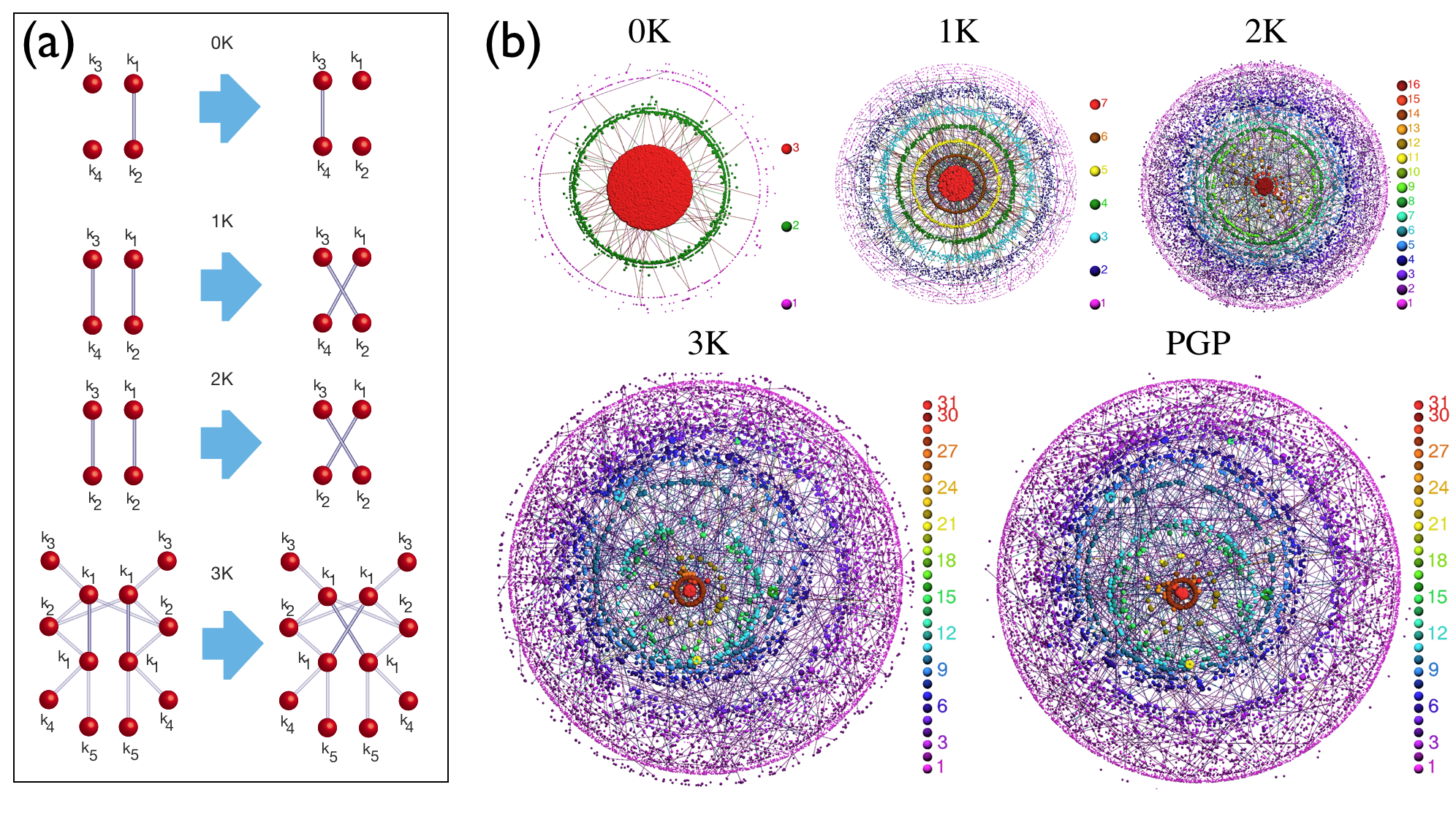
To answer these questions, we must compare a real network with typical random networks defined by its -distribution. If there is no difference between such -random networks and the real network, then the latter is fixed by its -distribution. To obtain a -random version of the real network, we -randomize it as illustrated in Fig. 1(a)—we randomly rewire (pairs of) links preserving the -distribution in the network, generalizing known network randomization techniques Maslov and Sneppen (2002); Maslov et al. (2003) used to compute motif statistical significance. The result of this -randomization procedure are random networks that have the same -distribution as the original real network, but that are maximally random in all other respects.
Our question thus becomes what is the minimum value of such that there is no difference between a real network and its -randomizations? It seems at first that the answer to this question should strongly depend on the specific networks we consider.
We consider a variety of social, biological, transportation, communication, and technological networks, see Section III. Although the -series applies to directed and even annotated networks Dimitropoulos et al. (2009), here we report results for undirected networks. The -distributions for directed or annotated networks contain more information than for undirected networks. Therefore, -series converges faster in the former case Dimitropoulos et al. (2009). Below we show the results for the well-studied social web of trust relationships extracted from Pretty Good Privacy (PGP) data Boguñá et al. (2004). We obtain similar results for all other considered networks (protein interactions in Saccharomyces cerevisiae, scientific collaborations, US air transportation, and the Internet), except for the power grid, see Section IV, where we also discuss possible reasons for why the power grid appears as an exception.
Fig. 1(b) visualizes the PGP network and its -randomizations. We observe that the -series converges at . While the -random network has little in common with the real network, the -random one is somewhat more similar, even more so for , and there is very little difference between the real PGP network and its -random counterpart.
To provide a more detailed and insightful comparison between the real network and its -randomizations, we compute a variety of metrics for each. Some popular metrics, such as degree distribution, average nearest neighbor connectivity, clustering, etc., are functions, sometimes peculiar, of -distributions, and therefore it is not surprising that they are properly captured by -series, as we confirm in Section IV.1. We classify metrics that do not explicitly depend on -distributions as microscopic, mesoscopic, and macroscopic. We choose them to probe the network structure at the local, medium, and global scales.
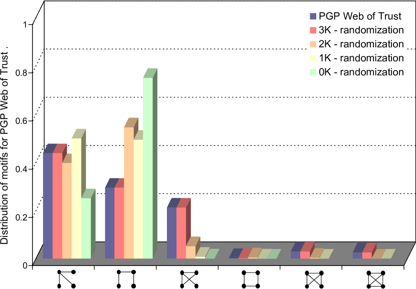
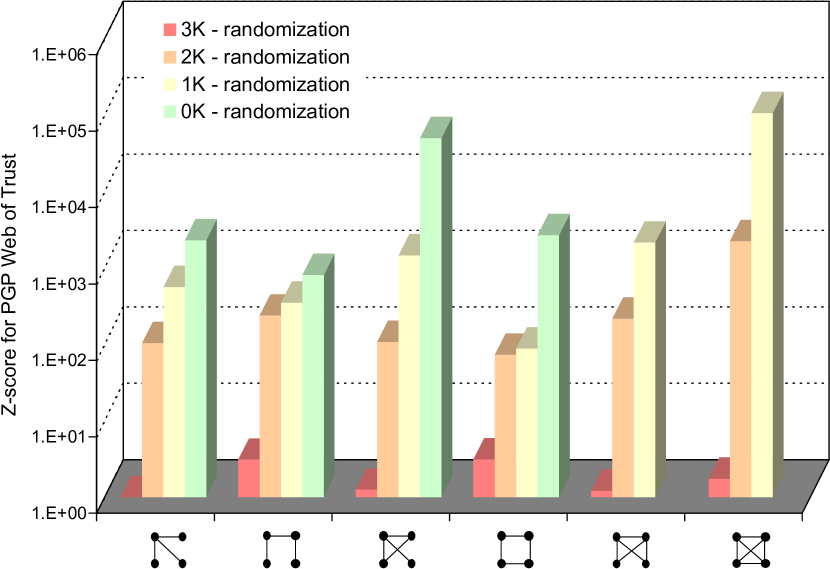
The simplest microscopic, local-structure statistics, which are not fixed by the -distributions with , are the frequencies of motifs of size without degree information. We compute these frequencies in the real network and its -randomizations, and show the results in Fig. 2. We find that no motif is statistically significant for , i.e., all the Z-scores are small, and all the motif frequencies in the real network and its -randomization are virtually the same.
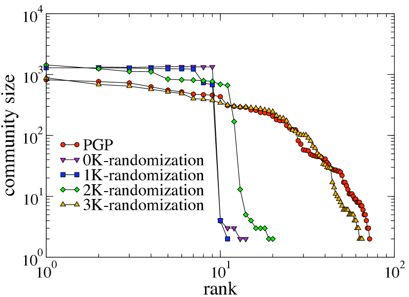
At the mesoscopic scale, we consider the community structure of the PGP network. A community is a subgraph with many internal connections, and a relatively small number of connections external to the subgraph. Fig. 3 shows that the community structure is indeed a “mesoscopic” metric because the community sizes range from a few nodes to thousands of nodes for largest communities. Fig. 3 shows that the community size distributions in the PGP network and its -randomization are very similar.
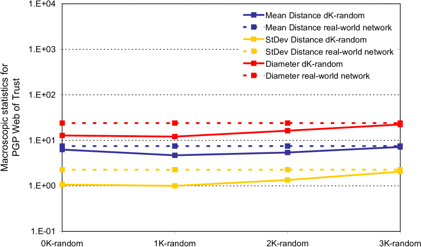
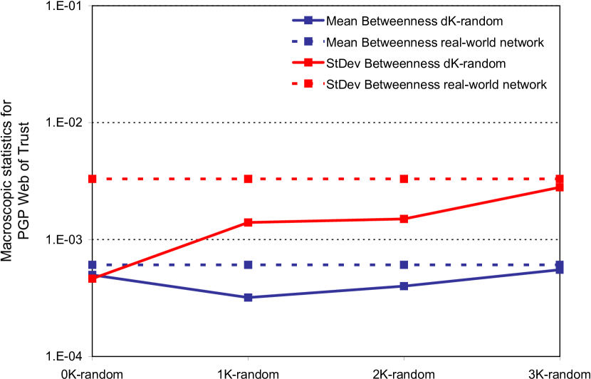
At the macroscopic scale, we consider two popular and important statistics that depend on a network’s global structure: the node betweenness centrality and the distribution of lengths of shortest paths in a network. Fig. 4 once again shows that is sufficient to capture even such global graph properties; the considered metrics are approximately the same for the PGP network and its -randomization.
We call a given real network -random if all its metrics, at all scales from local to global, are approximately the same as the corresponding metrics in its -randomizations. We see in Section IV that in agreement with the results of Vázquez et al. Vázquez et al. (2004), almost all networks that we collected data for are -random at most (some networks are - or even -random). In other words, the global structure of these networks is captured entirely by the distribution of node triples and their degrees.
It is an open question why many different real networks are -random. A trivial answer would be that is just “constraining enough.” There may only be a few possible rewirings preserving the -distribution. But why exactly is sufficient for real networks? There are many classes of synthetic graphs, such as latices, for which no substantially smaller than the graph size is “constraining enough.” Perhaps the answer can be obtained by studying the hidden metric spaces underlying real networks Boguñá et al. (2009). The distances in such spaces abstract intrinsic similarities between nodes. If these spaces are metric—and we have found empirical evidence that they are indeed such Serrano et al. (2008)—then the triangle inequality naturally yields and explains network clustering, which the -distribution captures by definition.
Regardless of the actual explanation, our results have diverse implications. First, our -randomization basis makes it clear that there is no a priori preferred null model for network randomization. To tell how statistically important a given motif is, it is necessary to compare its frequency in the real network with its frequency in a network randomization, a null model. But one can -randomize any network for any , and we find that the (relative) statistical significance of motifs strongly depends on for all the considered networks. Therefore choosing any specific value of , or more generally, any specific null model to compute motif significance requires some non-trivial justification.
Second, our finding that many networks are -random can assist our understanding of how functions of an evolving network shape its structure. Indeed, one can potentially simplify such explanations to how the observed -distribution has emerged in the network. As soon as one explains the emergence of the -distribution, all other structural properties of the network follow as a consequence of its -randomness.
Finally, our work has practical implications for the design of network topology models and generators. Many scientific disciplines, including biology Kuo et al. (2006); den Bulcke et al. (2006); Knabe et al. (2008b); Roy et al. (2008) and computer science Waxman (1988); Zegura et al. (1996); Medina et al. (2001); Winick and Jamin (2002), require laboratory modeling of real networks, and in particular the ability to generate random graphs that reproduce their important structural properties. Experimentation with the -series representation of real networks has revealed its theoretical and practical strengths for this task—one can reproduce all important structural properties of a given network by generating its -random graphs. Recent work Dimitropoulos et al. (2009) extending the -series construction to support rich semantic, structural, or functional annotations of nodes and links in real networks suggests a considerable untapped potential of -series for many disciplines.
II The -series illustrated
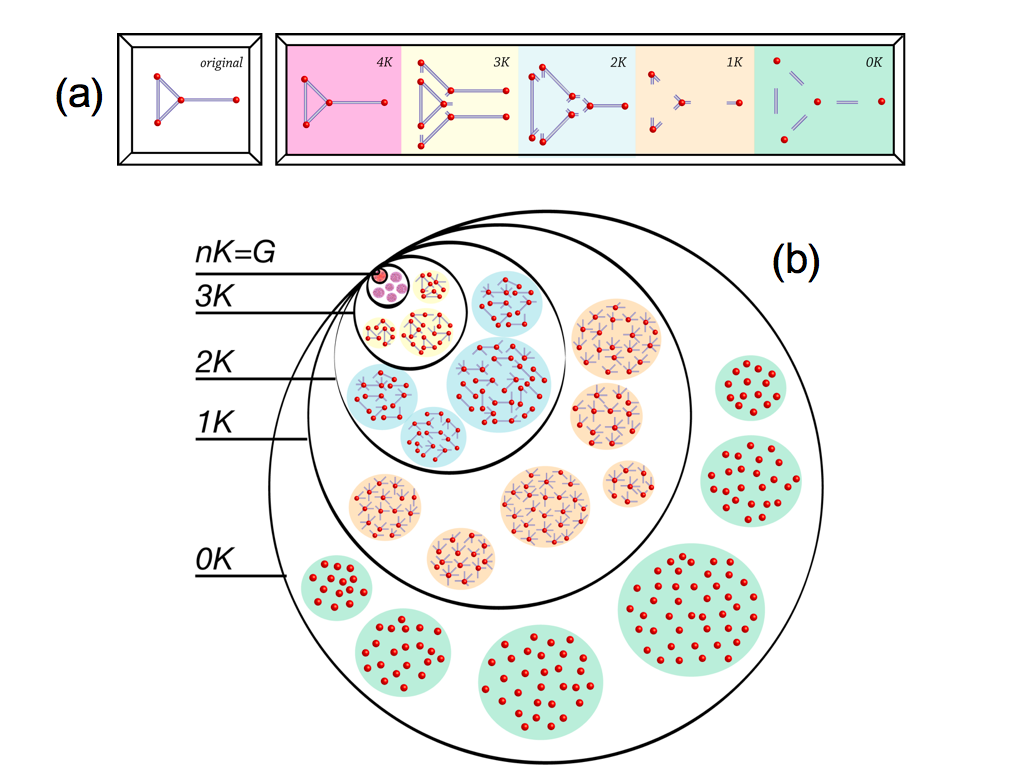
In Fig. 5(a) we illustrate -series for a graph of size . The -distribution is the graph itself. The -distribution consists of its three subgraphs of size : one triangle connecting nodes of degrees , , and , and two wedges connecting nodes of degrees , , and . The -distribution is the joint degree distribution in the graph. It specifies the number of links (subgraphs of size ) connecting nodes of different degrees: one link connects nodes of degrees and , two links connect nodes of degrees and , and one link connects nodes of degree and . The -distribution is the degree distribution in the graph. It lists the number of nodes (subgraphs of size ) of different degree: one node of degree , two nodes of degree , and one node of degree . The -distribution is just the average degree in the graph, which is .
Fig. 5(b) illustrates the inclusiveness and convergence of -series by showing the hierarchy of -graphs, which are graphs that have the same -distribution as some graph of size . The black circles schematically shows the sets of -graphs.
The set of -graphs is largest: the number of different graphs that have the same average degree as is enormous. These graphs may have a structure drastically different from ’s. The set of -graphs is a subset of -graphs, because each graph with the same degree distribution as in has also the same average degree as , but not vice versa. As a consequence, typical (“maximally random”) -graphs tend to be more similar to than -graphs. The set of -graphs is a subset of -graphs, also containing .
As increases, the circles become smaller because the number of different -graphs decreases. Since all the -graph sets contain , the circles “zoom-in” on it, and while their number decreases, -graphs become increasingly more similar to . In the limit, the set of -graphs consists of only one element, itself.
III The real networks considered
We collected data for a number of real networks. We wanted the set of considered networks to be representative, in the sense that it should contain networks of different nature, coming from different domains, thus showing the universality of our -basis. The considered networks include social, biological, transportation, and technological networks. Specifically, we report results for:
-
•
The social web of trust relationships among people. The trust relationships are inferred using the data from the Pretty Good Privacy (PGP) encryption algorithm Boguñá et al. (2004). We extract the strongly connected component from this network. The nodes are people, and there is a link between two people if they trust each other.
-
•
The social network of scientific collaborations extracted from the arXiv condensed-matter database Newman (2001). The nodes are authors, and there is a link between two authors if they co-authored a paper.
-
•
The biological network of protein interactions in the yeast Saccharomyces cerevisiae collected from the database of interacting proteins Colizza et al. (2006). The nodes are proteins, and there is a link between two proteins if they interact.
-
•
The US air transportation network Colizza et al. (2007). The nodes are airports, and there is a link between two airports if there is a direct flight between them.
-
•
The topology of the Internet at the level of Autonomous Systems (ASs) Mahadevan et al. (2006b). The nodes are ASs, i.e., organizations owing parts of the Internet infrastructure, and there is a link between two ASs if they are physically connected.
-
•
The electrical power grid in the western US Watts and Strogatz (1998). The nodes are generators, transformers, or substations, two of which are linked if there is a high-voltage transmission line between them.
Table 1 lists these networks and their abbreviations used in the subsequent figures and tables.
| Network | Abbreviation |
|---|---|
| PGP Web of Trust Boguñá et al. (2004) | PGP |
| Scientific collaboration network Newman (2001) | Collab. |
| Protein interaction network Colizza et al. (2006) | Protein |
| US air transportation network Colizza et al. (2007) | Air |
| Internet at the level of ASs Mahadevan et al. (2006b) | Internet |
| Power grid in the western US Watts and Strogatz (1998) | Power |
IV Topologies of real networks and their -randomizations
In this section we compare the real networks to their -randomizations across a number of topological metrics.
IV.1 Metrics defined by -distributions
We first consider the most basic metrics, which are defined by the appropriate -distributions. Therefore it is not surprising that -random graphs with appropriate have the values of these metrics equal exactly to those in the real networks. Nevertheless, we report these results for consistency and illustration purposes.
IV.1.1 : degree distribution
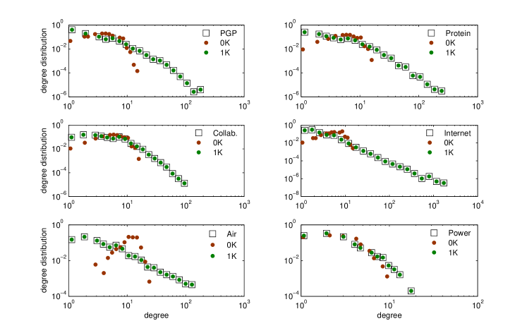
Fig. 6 shows the distributions of node degrees :
| (1) |
where is the number of nodes of degree in the network, and is the total number of nodes in it, so that is normalized, (we do not consider nodes of degree ). The -distribution fully defines the -distribution, i.e., the average degree in the network, by
| (2) |
but not vice versa.
We observe in Fig. 6 that while -randomizations are off, the -random graphs reproduce the degree distributions in the real networks exactly, which is by dentition: the -distribution is the degree distribution, and -randomization does not alter it. The -randomizations with do not alter the -distribution either, therefore they also match the degree distributions in the real networks exactly (not shown).
IV.1.2 : average neighbor degree
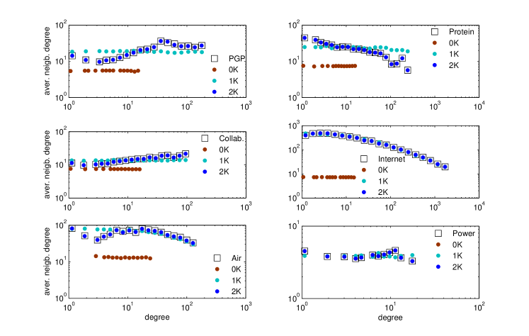
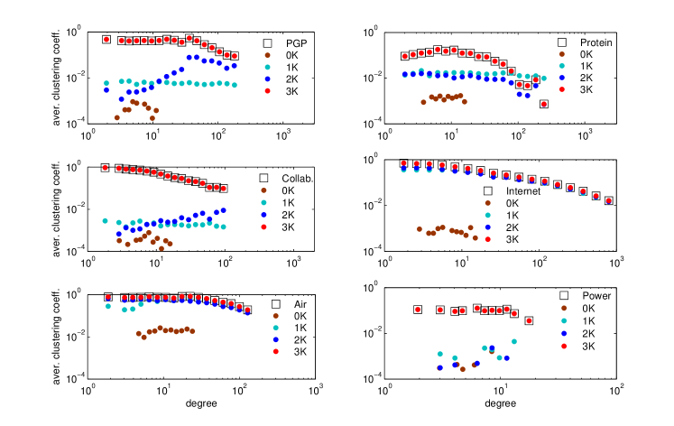
Fig. 7 shows the average degree of neighbors of nodes of degree . This function is a commonly used projection of the joint degree distribution (JDD) , i.e., the -distribution. The JDD is defined as
| (3) |
where is the number of links between nodes of degrees and in the network, is the total number of links in it, and
| (4) |
so that is normalized, . The -distribution fully defines the -distribution by
| (5) |
but not vice versa. The average neighbor degree is a projection of the -distribution via
| (6) |
We observe in Fig. 7 that while -randomizations are way off, the -randomization are much closer to the real networks, whereas the -randomizations have exactly the same average neighbor degrees as the real networks, which is again by definition: -randomization does not change . In the Internet case, even -randomization does not noticeably affect . The -randomizations with do not alter and consequently at all, therefore they reproduce the latter exactly as well for all the networks (not shown).
IV.1.3 : clustering
Fig. 8 shows degree-dependent clustering . Clustering of node is the number of triangles it forms, or equivalently the number of links among its neighbors, divided by the maximum such number, which is , where is ’s degree, . Averaging over all nodes of degree , the degree-dependent clustering is
| (7) |
The degree-dependent clustering is a commonly used projection of the -distribution. (See Serrano and Boguñá (2006a, b) for an alternative formalism involving three point correlations.)
The -distribution is actually two
distributions characterizing the concentrations of the two
non-isomorphic degree-labeled subgraphs of size , wedges and
triangles:
![]()
. Let be the number wedges involving nodes of degrees , , and , where is the central node degree, and let be the number of triangles consisting of nodes of degrees , , and , where is assumed to be symmetric with respect to all permutations of its arguments. Then the two components of the -distribution are
| (8) | |||||
| (9) |
where and are the total numbers of triangles and wedges in the network, and
| (10) |
so that both and are normalized, . The -distribution defines the -distribution (but not vice versa), by
| (11) | |||||
The normalization of - and -distributions implies the following identity between the numbers of triangles, wedges, edges, nodes, and the second moment of the degree distribution :
| (12) |
The degree-dependent clustering coefficient is the following projection of the -distribution
| (13) |
We observe in Fig. 8 that clustering in the real networks and their -randomizations with is exactly the same, which is again by definition. For , clustering differs drastically in many cases, except for the air transportation network and especially the Internet. Therefore we can say that the Internet is very close to being -random, i.e., fully defined by its degree distribution, as far as the -based metrics considered in this section are concerned. Neither -, -, nor even -randomization alter its -based (projection) metrics noticeably.
IV.2 Motifs and their Z-scores
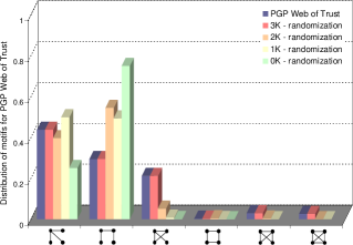
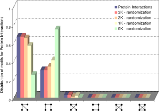
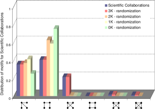
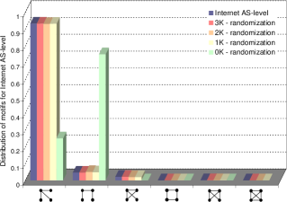
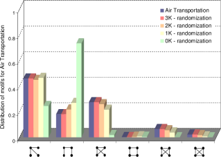
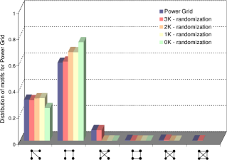
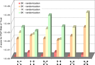
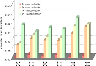
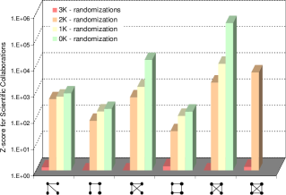
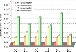
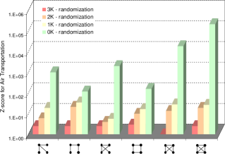
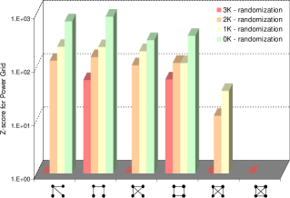
There are six non-isomorphic motifs of size , shown as the -axes in Figs. 9,10. For each network and for each , we obtain several -randomized samples of the network, and then for each motif we compute its distribution (normalized to the total number of subgraphs of size ) in the real network, and its average distribution in the -randomized samples of the network. The results are in Fig. 9. Fig. 10 reports the corresponding Z-scores. In certain cases, often for -randomizations, some motifs do not occur at all in any randomized samples, which explains the absence of some bars in the figures.
The key observation is that when the randomization null model is , the distributions of all motifs in the randomizations of all the networks except the power grid, are close to those in the real networks. The corresponding Z-scores are either low or zero. In other words, all motifs are statistically non-significant.
IV.3 Distance and betweenness distributions
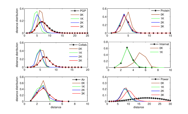
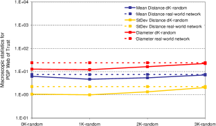
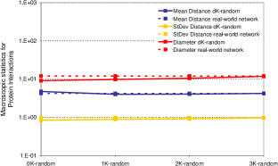
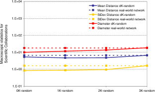
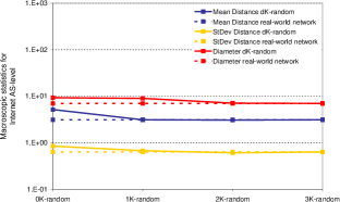
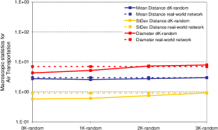
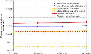
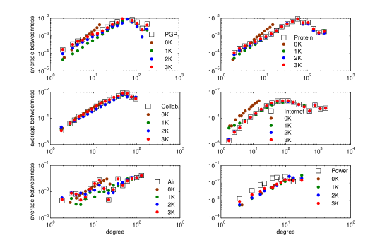
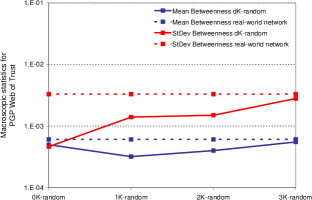
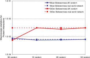
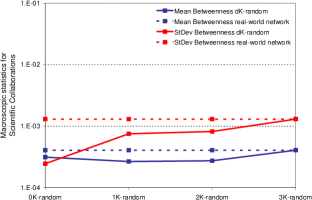
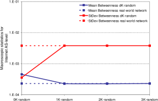
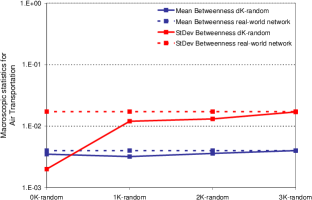
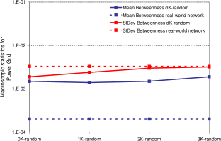
Fig. 11 shows the distance distribution in the real networks and in their -randomizations. The distance distribution is the distribution of hop-lengths of shortest paths between nodes in a network. Formally, if is the number of node pairs located at hop distance from each other, then the distance distribution is
| (14) |
where is the total number of nodes pairs in the network.
To provide a clearer view of how close the distance distributions in -randomizations are to the real networks, we show in Fig. 12 some scalar summary statistics of the distance distribution as functions of . These summary statistics are the average distance
| (15) |
and the standard deviation of the distance distribution . In addition we show in Fig. 12 the network diameter, i.e., the maximum hop-wise distance between nodes in the network, which is an extremal statistics of the distance distribution.
Fig. 13 shows degree-dependent betweenness centrality in the real networks and their -randomizations. Betweenness of node is a measure of how “important” is in terms of the number of shortest paths passing through it. Formally, if is the number of shortest paths between nodes and that pass through , and is the total number of shortest paths between the two nodes , then betweenness of is
| (16) |
Averaging over all nodes of degree , degree-dependent betweenness is
| (17) |
We also compute the betweenness distribution, and show its average and standard deviation in Fig. 14.
We observer similar trends with respect to both distance and betweenness metrics. The power grid cannot be approximated even by its -randomization. The Internet lies at the other extreme: even -randomization does not disturb its global metrics too much. The air transportation network appears to come next, as its -randomizations resemble it closely. But all the networks other than the power grid are very similar to their -randomizations.
IV.4 Scalar topological metrics and -randomness of real networks
| Metrics | PGP | Collab. | Protein | Air | Internet | Power |
|---|---|---|---|---|---|---|
| 4.6 | 6.4 | 6.4 | 11.9 | 6.3 | 4.7 | |
| 0.238 | 0.157 | -0.137 | -0.268 | -0.236 | -0.273 | |
| 0.27 | 0.65 | 0.09 | 0.62 | 0.46 | 0.68 | |
| 7.5 | 6.6 | 4.2 | 3.0 | 3.1 | 2.0 | |
| ? |
To conclude this section we show in Table 2 the most important scalar topological metrics for the real networks. These metrics are coarse summary statistics of the more informative and detailed metrics that we have considered in this section. Specifically, these coarse summaries are:
-
•
is the average degree in the network, Eq. (2), which is both the -distribution and a summary statistics of the -distribution in the -series terminology;
-
•
is the assortativity coefficient,
(18) which is nothing but the Pearson correlation coefficient of the -distribution ;
-
•
is the average clustering
(19) which is a coarse summary statistics of the -distribution;
-
•
is the average distance, Eq. (15), which is unrelated to -distributions;
-
•
is the average betweenness,
(20) unrelated to -distributions as well.
In Table 2 we also show the minimum value of such the -randomization null model approximately reproduces the real network with respect to all the metrics above.
The observation that the power grid cannot be approximated even by its -randomization is instructive. It shows that there are real networks for which no is capable of preserving the network structure upon -randomizing. In case of the power grid, the explanation why this network is not even -random may be related to the fact that it is designed and controlled by human engineers in a single organization. Informally, we can think of it as rather “non-random,” designed, and thus bearing a number of constraints that the -distributions with low cannot capture. Informally, the higher required to approximately preserve the network structure upon -randomization, the less “random” the network is. The commonly referred explanation that the power grid is an “outlier” because it is spatially embedded, may be less relevant here because two other networks that we have considered (the Internet and air transportation) are also spatially embedded.
What is different between the power grid and the other considered networks is that the latter are self-evolving. They may be engineered to a certain degree, such as the Internet, but their global structure and evolution are not fully controlled by any single human or organization. In the Internet case, for example, the global network topology is a cumulative effect of independent decisions made by tens of thousands of separate organizations, roughly corresponding to Autonomous Systems, i.e., nodes of the Internet graph.
In that sense, self-evolving complex networks are “more random.” However, why the level of their “randomness” is at remains an open question.
V Motif-based series vs. -series
In this section we compare -series with the series based on motifs, and show that the latter cannot form a systematic basis for topology analysis.
The difference between -series and motif-series, which we can call -series, is that the former is the series of distributions of -sized subgraphs labeled with node degrees in a given network, while the -series is the distributions of such subgraphs in which this degree information is ignored. This difference explains the mnemonic names for these two series: ‘’ in ‘’ refers to the subgraph size, while ‘’ signifies that they are labeled by node degrees—‘’ is a standard notation for node degrees.
This difference between the -series and -series is crucial. The -series are inclusive, in the sense that the -distribution contains the full information about the -distribution, plus some additional information, which is not true for -series.
| -statistics | -statistics | |
|---|---|---|
| - | ||
To see this, let us consider the first few elements of both series
in Table 3. In Section IV.1 we show
explicitly how the -distributions define the
-distribution for . The key observation is that the
-series does not have this property. The ’th element of
-series is undefined. For we have the number of subgraphs
of size , which is just , the number of nodes in the network.
For , the corresponding statistics is , the number of links,
subgraphs of size . Clearly, and are independent
statistics, and the former does not define the latter. For ,
the statistics are and , the total number of wedges and
triangles, subgraphs of size , in the network. These do not
define the previous element either. Indeed, consider the
following two networks of size
—the chain and the star:
![[Uncaptioned image]](/html/0908.1143/assets/x36.png)
There are no triangles in either network, . In the chain network, the number of wedges is , and in the star . We see that even though () scales completely differently with in the two networks, the number of edges () is the same.
In summary, -series is not inclusive. For each , the corresponding element of the series reflects a differen kind of statistical information about the network topology, unrelated or only loosely related to the information conveyed by the preceding elements. At the same time, similar to -series, the -series is also converging since at it specifies the whole network topology. However, this convergence is much slower that in the -series case. In the two networks considered above, for example, neither nor , fix the network topology as there are many non-isomorphic graphs with the same counts, whereas the -distributions and define the chain and star topologies exactly.
The node degrees thus provide necessary information about subgraph locations in the original network, which improves convergence, and makes the -series basis inclusive and systematic.
Acknowledgements.
We thank KC Claffy, Marina Fomenkov, Alex Arenas, and Alessandro Vespignani for useful comments and discussions, and Connie Lyu and Bradley Huffaker for their help with Figs. 1,5. This work was supported in part by DGES grant FIS2007-66485-C02-02, by NSF CNS-0434996 and CNS-0722070, by DHS N66001-08-C-2029, and by Cisco Systems.References
- Milo et al. (2002) R. Milo, S. Shen-Orr, S. Itzkovic, N. Kashtan, D. Chklovskii, and U. Alon, Science 298, 824 (2002).
- Alon (2007) U. Alon, Nat Rev Genet 8, 450 (2007).
- Alon (2006) U. Alon, An Introduction to Systems Biology: Design Principles of Biological Circuits (Chapman & Hall/CRC, Boca Raton, 2006).
- Rosenfeld et al. (2002) N. Rosenfeld, M. Elowitz, and U. Alon, J Mol Biol 323, 785 (2002).
- Mangana et al. (2006) S. Mangana, S. Itzkovitz, A. Zaslaver, and U. Alon, J Mol Biol 356, 1073 (2006).
- Knabe et al. (2008a) J. Knabe, C. Nehaniva, and M. Schilstra, Biosystems 94, 68 (2008a).
- Ingram et al. (2006) P. Ingram, M. Stumpf, and J. Stark, BMC Genomics 7, 108 (2006).
- Cordero and Hogeweg (2006) O. Cordero and P. Hogeweg, Mol Biol Evol 23, 1931 (2006).
- Kuo et al. (2006) P. Kuo, W. Banzhaf, and A. Leier, Biosystems 85, 177 (2006).
- Mazurie et al. (2005) A. Mazurie, S. Bottani, and M. Vergassola, Genome Biol 6, R35 (2005).
- Sakata et al. (2005) S. Sakata, Y. Komatsu, and T. Yamamori, Neurosci Res 51, 309 (2005).
- Vázquez et al. (2004) A. Vázquez, R. Dobrin, D. Sergi, J.-P. Eckmann, Z. N. Oltvai, and A.-L. Barabási, Proc Natl Acad Sci USA 101, 17940 (2004).
- Artzy-Randrup et al. (2004) Y. Artzy-Randrup, S. Fleishman, N. Ben-Tal, and L. Stone, Science 305, 1107 (2004).
- Mahadevan et al. (2006a) P. Mahadevan, D. Krioukov, K. Fall, and A. Vahdat, Comput Commun Rev 36, 135 (2006a).
- Boguñá et al. (2004) M. Boguñá, R. Pastor-Satorras, A. Díaz-Guilera, and A. Arenas, Phys Rev E 70, 056122 (2004).
- Alvarez-Hamelin et al. (2006) J. I. Alvarez-Hamelin, L. Dall’Asta, A. Barrat, and A. Vespignani, in Advances in Neural Information Processing Systems 18, edited by Y. Weiss, B. Schölkopf, and J. Platt (MIT Press, Boston, 2006) pp. 41–50.
- Maslov and Sneppen (2002) S. Maslov and K. Sneppen, Science 296, 910 (2002).
- Maslov et al. (2003) S. Maslov, K. Sneppen, and U. Alon, “Handbook of graphs and networks,” (Wiley-VCH, Berlin, 2003) Chap. Correlations Profiles and Motifs in Complex Networks.
- Dimitropoulos et al. (2009) X. Dimitropoulos, D. Krioukov, G. Riley, and A. Vahdat, ACM T Model Comput S 19, 17 (2009).
- Duch and Arenas (2005) J. Duch and A. Arenas, Phys Rev E 72, 027104 (2005).
- Freeman (1977) L. Freeman, Sociometry 40, 35 (1977).
- Boguñá et al. (2009) M. Boguñá, D. Krioukov, and kc claffy, Nature Physics 5, 74 (2009).
- Serrano et al. (2008) M. Á. Serrano, D. Krioukov, and M. Boguñá, Phys Rev Lett 100, 078701 (2008).
- den Bulcke et al. (2006) T. V. den Bulcke, K. V. Leemput, B. Naudts, P. van Remortel, H. Ma, A. Verschoren, B. D. Moor, and K. Marchal, BMC Bioinformatics 7 (2006).
- Knabe et al. (2008b) J. Knabe, C. Nehaniva, and M. Schilstra, Artif Life 14, 135 (2008b).
- Roy et al. (2008) S. Roy, M. Werner-Washburne, and T. Lane, Bioinformatics 24, 1318 (2008).
- Waxman (1988) B. M. Waxman, IEEE J Sel Area Comm 6, 1617 (1988).
- Zegura et al. (1996) E. Zegura, K. Calvert, and S. Bhattacharjee, in Proc INFOCOM, Vol. 2 (1996) pp. 594–602.
- Medina et al. (2001) A. Medina, A. Lakhina, I. Matta, and J. Byers, in Proc MASCOTS (2001) pp. 346–353.
- Winick and Jamin (2002) J. Winick and S. Jamin, Inet-3.0: Internet Topology Generator, Technical Report UM-CSE-TR-456-02 (University of Michigan, 2002).
- Newman (2001) M. E. J. Newman, Proc Natl Acad Sci USA 98, 404 (2001).
- Colizza et al. (2006) V. Colizza, A. Flammini, M. Á. Serrano, and A. Vespignani, Nat Phys 2, 110 (2006).
- Colizza et al. (2007) V. Colizza, R. Pastor-Satorras, and A. Vespignani, Nat Phys 3, 276 (2007).
- Mahadevan et al. (2006b) P. Mahadevan, D. Krioukov, M. Fomenkov, B. Huffaker, X. Dimitropoulos, kc claffy, and A. Vahdat, Comput Commun Rev 36, 17 (2006b).
- Watts and Strogatz (1998) D. J. Watts and S. H. Strogatz, Nature 393, 440 (1998).
- Serrano and Boguñá (2006a) M. Á. Serrano and M. Boguñá, Phys Rev E 74, 056114 (2006a).
- Serrano and Boguñá (2006b) M. A. Serrano and M. Boguñá, Phys Rev E 74, 056115 (2006b).