Community detection algorithms: a comparative analysis

Abstract

Uncovering the community structure exhibited by real networks is a crucial step towards an understanding of complex systems that goes beyond the local organization of their constituents. Many algorithms have been proposed so far, but none of them has been subjected to strict tests to evaluate their performance. Most of the sporadic tests performed so far involved small networks with known community structure and/or artificial graphs with a simplified structure, which is very uncommon in real systems. Here we test several methods against a recently introduced class of benchmark graphs, with heterogeneous distributions of degree and community size. The methods are also tested against the benchmark by Girvan and Newman and on random graphs. As a result of our analysis, three recent algorithms introduced by Rosvall and Bergstrom, Blondel et al. and Ronhovde and Nussinov, respectively, have an excellent performance, with the additional advantage of low computational complexity, which enables one to analyze large systems.

I Introduction

The modern science of networks is probably the most active field within the new interdisciplinary science of complex systems. Many complex systems can be represented as networks, where the elementary parts of a system and their mutual interactions are nodes and links, respectively Newman (2003); Boccaletti et al. (2006). Complex systems are usually organized in compartments, which have their own role and/or function. In the network representation, such compartments appear as sets of nodes with a high density of internal links, whereas links between compartments have a comparatively lower density. These subgraphs are called communities, or modules, and occur in a wide variety of networked systems Girvan and Newman (2002); Fortunato (2009).

Finding compartments may shed light on the organization of complex systems and on their function. Therefore detecting communities in networks has become a fundamental problem in network science. Many methods have been developed, using tools and techniques from disciplines like physics, biology, applied mathematics, computer and social sciences. However, it is still not clear which algorithms are reliable and shall be used in applications. The question of the reliability itself is tricky, as it requires shared definitions of community and partition which are, at present, still missing. This essentially means that, despite the huge literature on the topic, there is still no agreement among scholars on what a network with communities looks like. Nevertheless, there has been a silent acceptance of a simple network model, the planted $\ell$-partition model Condon and Karp (2001), which is often used in the literature in various versions. In this model one “plants” a partition, consisting of a certain number of groups of nodes. Each node has a probability $p_{in}$ of being connected to nodes of its group and a probability $p_{out}$ of being connected to nodes of different groups. As long as $p_{in}>p_{out}$ the groups are communities, whereas when $p_{in}\leq p_{out}$ the network is essentially a random graph, without community structure. The most popular version of the planted $\ell$-partition model was proposed by Girvan and Newman (GN benchmark) Girvan and Newman (2002). Here the graph consists of $128$ nodes, each with expected degree $16$, which are divided into four groups of $32$. The GN benchmark is regularly used to test algorithms for community detection. Indeed, algorithms can be compared based on their performance on this benchmark. This has been done by Danon et al. Danon et al. (2005). However, the GN benchmark has two drawbacks: 1) all nodes have the same expected degree; 2) all communities have equal size. These features are unrealistic, as complex networks are known to be characterized by heterogeneous distributions of degree Albert et al. (1999); Newman (2003); Boccaletti et al. (2006) and community sizes Palla et al. (2005); Guimerà et al. (2003); Danon et al. (2007); Clauset et al. (2004); Lancichinetti et al. (2009). In recent papers Lancichinetti et al. (2008); Lancichinetti and Fortunato (2009), we have introduced a new class of benchmark graphs (LFR benchmark), that generalize the GN benchmark by introducing power law distributions of degree and community size. The new graphs are a real generalization, in that the GN benchmark is recovered in the limit case in which the exponents of the distributions of degree and community sizes go to infinity. Most community detection algorithms perform very well on the GN benchmark, due to the simplicity of its structure. The LFR benchmark, instead, poses a much harder test to algorithms, and makes it easier to disclose their limits. Moreover, the LFR benchmark graphs can be built very quickly: the complexity of the construction algorithms is linear in the number of links of the graph, so one can perform tests on very large systems, provided the method at study is fast enough to analyze them.

For these reasons, we believe that a serious assessment of the goodness of community detection algorithms can be made by evaluating their performance on the LFR benchmark. In this paper we propose a comparative analysis of this kind. After explaining briefly the LFR benchmark and how to compare partitions quantitatively we will pass to the description the algorithms that we examined. We will present the analysis of the algorithms’ performance first on the GN benchmark and then on the LFR benchmark, in its various versions including weighted and directed graphs, along with graphs with overlapping communities. Finally we will consider the issue of whether the algorithms are able to give a null result, i. e. how they handle networks without expected community structure, like random graphs. Our analysis will reveal that there are, at present, algorithms which are fast and reliable in many situations. We will conclude with a summary of our results and their consequences.

II The LFR benchmark

The LFR benchmark Lancichinetti et al. (2008); Lancichinetti and Fortunato (2009) is a special case of the planted $\ell$-partition model, in which groups are of different sizes and nodes have different degrees. The node degrees are distributed according to a power law with exponent $\tau_{1}$; the community sizes also obey a power law distribution, with exponent $\tau_{2}$. In the following, $N$ indicates the number of nodes of the network. In the construction of the benchmark graphs, each node receives its degree once and for all, and keeps it fixed until the end. In this way, the two parameters $p_{in}$ and $p_{out}$ of the planted $\ell$-partition model in this case are not independent. Once the value of $p_{in}$ is set one obtains the value of $p_{out}$ and viceversa. It is more practical to choose as independent parameter the mixing parameter $\mu$, which expresses the ratio between the external degree of a node with respect to its community and the total degree of the node. Of course, in general one may take different values for the mixing parameter for different nodes, but we will assume, for simplicity, that $\mu$ is the same for all nodes, consistently with the standard hypotheses of the planted $\ell$-partition model. By construction, the groups are communities when $p_{in}>p_{out}$. This condition can be translated into a condition on the mixing parameter $\mu$. Let us label $k_{i}^{in}$ and $k_{i}^{out}$ the internal and external degree of node $i$ with respect to its community (which we denote with $c$). By definition, $k_{i}^{in}$ is the number of neighbors of $i$ that belong to its community $c$ and $k_{i}^{out}$ the number of neighbors of $i$ that belong to the other communities. The number of available connections $k_{c}^{out}$ ($k_{c}^{in}$) outside (inside) $c$ is given by the sum of the degrees of the nodes outside (inside) the community. If the numbers of nodes inside and outside $c$ are not too small, the sum of their degrees can be approximated by the product of the average degree $\langle k\rangle$ by the number of nodes. We indicate with $n_{c}$ the number of nodes of the community $c$ of node $i$, so we have that $k_{c}^{out}\sim(N-n_{c})\langle k\rangle$ and $k_{c}^{in}\sim n_{c}\langle k\rangle$. By definition of the linking probabilities $p_{in}$ and $p_{out}$ we deduce that

$$p_{out}=\frac{k_{i}^{out}}{k_{c}^{out}}\sim\frac{k_{i}^{out}}{(N-n_{c})\langle k\rangle},$$ (1)

and

$$p_{in}=\frac{k_{i}^{in}}{k_{c}^{in}}\sim\frac{k_{i}^{in}}{n_{c}\langle k\rangle}.$$ (2)

In this way, the condition for the existence of communities $p_{in}>p_{out}$ becomes

$$\frac{k_{i}^{in}}{n_{c}\langle k\rangle}>\frac{k_{i}^{out}}{(N-n_{c})\langle k\rangle},$$ (3)

from which we get

$$k_{i}^{in}>\frac{n_{c}k_{i}^{out}}{N-n_{c}}.$$ (4)

On the other hand, by definition we have that

$$\mu=\frac{k_{i}^{out}}{k_{i}^{in}+k_{i}^{out}}.$$ (5)

By comparing Eq. 5 with Eq. 4 we obtain the desired condition on $\mu$

$$\mu<\frac{N-n_{c}}{N}.$$ (6)

The condition expressed in Eq. 6 is general, and applies to any version of the planted $\ell$-partition model. When communities are different in size, the upper bound on $\mu$ depends on the specific community at hand. However, if $n_{c}^{max}$ is the size of the largest community, we can safely assume that, whenever $\mu<(N-n_{c}^{max})/N$, all communities are well defined. In the GN benchmark, where $n_{c}=32$ and $128$, the condition becomes $\mu<3/4$. This is interesting, as in most works using the GN benchmark, one usually assumes that communities are there as long as $\mu<1/2$, whereas they are not well defined for $\mu>1/2$. Instead, we see that communities are there, at least in principle, up until $\mu=3/4$. However, we stress that, even if communities are there, methods may be unable to detect them. The reason is that, due to fluctuations in the distribution of links in the graphs, already before the limit imposed by the planted partition model it may be impossible to detect the communities and the model graphs may look similar to random graphs. This issue of the actual significance of communities and their detectability a priori is very important and has been recently discussed in the literature Reichardt and Leone (2008); Bianconi et al. (2009); Lancichinetti et al. (2009). We notice that, on large networks, when $n_{c}\ll N$, the limit value of $\mu$ below which communities are defined approaches $1$. In our tests with the LFR benchmark, we will often be in this regime.

III Comparing partitions

Testing an algorithm on any graph with built-in community structure also implies defining a quantitative criterion to estimate the goodness of the answer given by the algorithm as compared to the real answer that is expected. This can be done by using suitable similarity measures. For reviews of similarity measures see Refs. Fortunato and Castellano (2009); Meilă (2007); Traud et al. (2008). In the first tests of community detection algorithms, one used a measure called fraction of correctly identified nodes, introduced by Girvan and Newman Girvan and Newman (2002). However, it is not well defined in some cases (e. g. when a detected community is a merger of two or more “real” communities), so in the last years other measures have been used. In particular, measures borrowed from information theory have proved to be reliable.

To evaluate the Shannon information content Mackay (2003) of a partition, one starts by considering the community assignments $\{x_{i}\}$ and $\{y_{i}\}$, where $x_{i}$ and $y_{i}$ indicate the cluster labels of vertex $i$ in partition ${\cal X}$ and ${\cal Y}$, respectively. One assumes that the labels $x$ and $y$ are values of two random variables $X$ and $Y$, with joint distribution $P(x,y)=P(X=x,Y=y)=n_{xy}/n$, which implies that $P(x)=P(X=x)=n_{x}^{X}/n$ and $P(y)=P(Y=y)=n_{y}^{Y}/n$, where $n_{x}^{X}$, $n_{y}^{Y}$ and $n_{xy}$ are the sizes of the clusters labeled by $x$, $y$ and of their overlap, respectively. The mutual information $I(X,Y)$ of two random variables is defined as

$$I(X,Y)=\sum_{x}\sum_{y}P(x,y)\log\frac{P(x,y)}{P(x)P(y)}.$$ (7)

The measure $I(X,Y)$ tells how much we learn about $X$ if we know $Y$, and viceversa. Actually $I(X,Y)=H(X)-H(X|Y)$, where $H(X)=-\sum_{x}P(x)\log P(x)$ is the Shannon entropy of $X$ and $H(X|Y)=-\sum_{x,y}P(x,y)\log P(x|y)$ is the conditional entropy of $X$ given $Y$. The mutual information is not ideal as a similarity measure: in fact, given a partition ${\cal X}$, all partitions derived from ${\cal X}$ by further partitioning (some of) its clusters would all have the same mutual information with ${\cal X}$, even though they could be very different from each other. In this case the mutual information would simply equal the entropy $H(X)$, because the conditional entropy would be systematically zero. To avoid that, Danon et al. adopted the normalized mutual information Danon et al. (2005)

$$I_{norm}({\cal X},{\cal Y})=\frac{2I(X,Y)}{H(X)+H(Y)},$$ (8)

which equals $1$ if the partitions are identical, whereas it has an expected value of $0$ if the partitions are independent. The normalized mutual information is currently very often used in tests of community detection algorithms. We have recently proposed a definition of the measure to evaluate the similarity of covers, i. e. of divisions of the network in overlapping communities, which one needs for the tests of Section VI.4. The details can be found in the Appendix of Ref. Lancichinetti et al. (2009). We stress that our definition is not a proper extension of the normalized mutual information, in the sense that it does not recover exactly the same value of the original measure for the comparison of proper partitions without overlap, even though the values are close. For consistency we used our definition in all tests, although in the tests involving benchmarks without overlapping communities the classic expression of Eq. 8 could be used. For this reason, we warn that in the plots showing the performance of the algorithms on the GN benchmark, the curves are not identical to those already seen in previous papers (for, e. g., modularity-based methods), where Eq. 8 was used, although they are rather close.

IV The algorithms

We have tested a wide spectrum of community detection methods. In some cases the software to implement the algorithms was publicly available, in other cases the original developers have let us use their own code, otherwise we have created the software on our own. We wanted to have a representative subset of algorithms, that exploit some of the most interesting ideas and techniques that have been developed over the last years. Obviously we could not by any means perform an analysis of all existing techniques, as their number is huge. Some of them were excluded a priori, if particularly slow, as our tests involve graphs with a few thousand nodes, which old methods are unable to handle. On the other hand, the code to create the LFR benchmark is freely available note1 and scholars are welcome to test their algorithms on it and compare their performance with that of the algorithms analyzed here. Here is the list of the algorithms we considered.

• Algorithm of Girvan and Newman Girvan and Newman (2002); Newman and Girvan (2004). It is the first algorithm of the modern age of community detection in graphs. It is a hierarchical divisive algorithm, in which links are iteratively removed based on the value of their betweenness, which expresses the number of shortest paths between pairs of nodes that pass through the link. In its most popular implementation, the procedure of link removal ends when the modularity of the resulting partition reaches a maximum. The modularity of Newman and Girvan is a well known quality function that estimates the goodness of a partition based on the comparison between the graph at hand and a null model, which is a class of random graphs with the same expected degree sequence of the original graph. The algorithm has a complexity $O(N^{3})$ on a sparse graph. In the following we will refer to it as GN.

• Fast greedy modularity optimization by Clauset, Newman and Moore Clauset et al. (2004). This method is essentially a fast implementation of a previous technique proposed by Newman Newman (2004). Starting from a set of isolated nodes, the links of the original graph are iteratively added such to produce the largest possible increase of the modularity of Newman and Girvan at each step. The fast version of Clauset, Newman and Moore, which uses more efficient data structures, has a complexity of $O(N\log^{2}N)$ on sparse graphs.

• Exhaustive modularity optimization via simulated annealing Guimerà et al. (2004); Massen and Doye (2005); Medus et al. (2005); Guimerà and Amaral (2005). The goal is the same as in the previous algorithm, but the precision of the final estimate of the maximum is far higher, due to the exhaustive optimization, at the expense of the computational speed. The latter cannot be expressed in closed form, as in the cases above, as it depends on the parameters used for the optimization. We will stick to the procedure used by Guimerá and Amaral Guimerà and Amaral (2005).

• Fast modularity optimization by Blondel et al. Blondel et al. (2008). This is a multistep technique based on a local optimization of Newman-Girvan modularity in the neighborhood of each node. After a partition is identified in this way, communities are replaced by supernodes, yielding a smaller weighted network. The procedure is then iterated, until modularity (which is always computed with respect to the original graph) does not increase any further. This method offers a fair compromise between the accuracy of the estimate of the modularity maximum, which is better than that delivered by greedy techniques like the one by Clauset et al. above, and computational complexity, which is essentially linear in the number of links of the graph.

• Algorithm by Radicchi et al. Radicchi et al. (2004). This algorithm is in the spirit of that by Girvan and Newman above. In fact, it is a divisive hierarchical method, where links are iteratively removed based on the value of their edge clustering coefficient, which is defined as the ratio between the number of loops based on the link and the largest possible number of loops that can be based on the link. The edge clustering coefficient is a local measure, so its computation is not so heavy as that of edge betweenness, which yields a significant improvement in the complexity of the algorithm, which is $O(N^{2})$ on a sparse graph. Another major difference from the GN algorithm is the stopping criterion of the procedure, which depends on the properties of the communities themselves and not on the values of a quality function like modularity. Radicchi et al. considered two types of communities: strong communities are groups of nodes such that the internal degree of each node exceeds its external degree; weak communities are groups of nodes such that the total internal degree of the nodes of the group exceeds their total external degree.

• Cfinder Palla et al. (2005). This is a local algorithm proposed by Palla et al. that looks for communities that may overlap, i.e. share nodes. It was the first paper in the physics literature on community detection to address this problem, which is important in many systems like, e. g., social networks. Communities are defined as the largest possible subgraphs that can be explored by rolling $k$-cliques across the network, where a $k$-clique rolls by rotating about any of its component $(k-1)$-cliques (which are links when $k=3$). The complexity of this procedure can be high, as the computational time needed to find all $k$-cliques of a graph is an exponentially growing function of the graph size Bron and Kerbosch (1973), but in practical applications the method is rather fast, enabling one to analyze systems with up to $10^{5}$ nodes.

• Markov Cluster Algorithm van Dongen (2000). This is an algorithm developed by S. Van Dongen, which simulates a peculiar diffusion process on the graph. One starts from the right stochastic matrix (or diffusion matrix) of the graph, which is obtained from the adjacency matrix of the original graph by dividing the elements of each row by their sum. Then one computes an integer power of this matrix (usually the square), which yields the probability matrix of a random walk after a number of steps equal to the number of powers of the right stochastic matrix considered. This step is called expansion. Next, each element of the matrix is raised to some power $\alpha$, in order to enhance (artificially) the probability of the walker to be trapped within a community. This step is called inflation. The expansion and inflation steps are iterated until one obtains the adjacency matrix of a forest (i. e. a disconnected tree), whose components are the communities. This method, widely used in bioinformatics, is strongly dependent on the choice of the parameter $\alpha$. Its complexity can be lowered to $O(Nk^{2})$ if, after each inflation steps, only the $k$ largest elements of the resulting matrix are kept, whereas the others are set to zero. In the following we will refer to the method as MCL.

• Structural algorithm by Rosvall and Bergstrom Rosvall and Bergstrom (2007). Here the problem of finding the best cluster structure of a graph is turned into the problem of optimally compressing the information on the structure of the graph, so that one can recover as closely as possible the original structure when the compressed information is decoded. This is achieved by computing the minimum of a function which expresses the best tradeoff between the minimal conditional information between the original and the compressed information (maximal faithfulness to the original information) and the maximal compression (least possible information to transmit). The optimization of the function is carried out via simulated annealing, which makes the algorithm quite slow, although one could always go for a faster and less accurate optimization. In the following we will refer to the method as Infomod.

• Dynamic algorithm by Rosvall and Bergstrom Rosvall and Bergstrom (2008). This technique is based on the same principle as the previous one. The difference is that before one was compressing the information on the structure of the graph, here one wishes to compress the information of a dynamic process taking place on the graph, namely a random walk. The optimal compression is achieved again by optimizing a quality function, which is the Minimum Description Length Rissanen (1978); Grünwald et al. (2005) of the random walk. Such optimization can be carried out rather quickly with a combination of greedy search and simulated annealing. In the following we will refer to the method as Infomap.

• Spectral algorithm by Donetti and Muñoz Donetti and Muñoz (2004). This is a method based on spectral properties of the graph. The idea is that eigenvector components corresponding to nodes in the same community should have similar values, if communities are well identified. Donetti and Muñoz focused on the eigenvectors of the Laplacian matrix. They considered a limited number of eigenvectors, say $g$, and represented each node of the graph as a geometric point in an Euclidean $g$-dimensional space, whose coordinates are the eigenvector components corresponding to the node. The points are then grouped with traditional hierarchical clustering techniques. Of the resulting partitions, one picks the one that maximizes the modularity by Newman and Girvan. The method is rather quick when only a few eigenvectors are computed, which is usually the case, as this can be done via the Lanczos method Lanczos (1950). In the following we will refer to the method as DM.

• Expectation-maximization algorithm by Newman and Leicht Newman and Leicht (2007). Here Bayesian inference is used to deduce the best fit of a given model to the data represented by the actual graph structure. The goodness of the fit is expressed by a likelihood that is maximized by means of the expectation-maximization technique Dempster et al. (1977). This leads to a system of self-consistent equations, that can be solved by iteration starting from suitable initial conditions. The equations can be solved rather quickly and fairly large systems can be analyzed in this way (up until $10^{6}$ nodes). A nice feature of the method is that it finds the most relevant group structure of the graph, whether the groups are communities or not (in graphs with multipartite structure the classes are rather anti-communities, as there are very few links inside the groups). A drawback of the method is the fact that one needs to feed the number of groups, which is usually not known a priori. In the following we will refer to the method as EM.

• Potts model approach by Ronhovde and Nussinov Ronhovde and Nussinov (2009). This method is based on the minimization of the Hamiltonian of a Potts-like spin model, where the spin state represents the membership of the node in a given community. A resolution parameter enables one to span several community scales, from very small to very large communities. The relevant scales are identified by checking for the stability of the partitions obtained for given values of the resolution parameter. This is done by computing the similarity of partitions obtained for the same resolution parameter but starting from different initial conditions. Peaks in the similarity spectrum correspond to stable/relevant partitions. The method is rather fast, its complexity is slightly superlinear in the number of links of the graph. In the following we will refer to the method as RN.

V Tests on the GN benchmark

Figure 1: Tests of the algorithms on the GN benchmark.

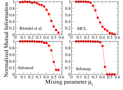
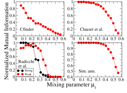
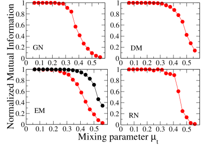
We begin by showing the performance of the algorithms on the GN benchmark. As we have explained in Section II, for the GN benchmark communities are well defined (in principle) up until a value $3/4=0.75$ for the mixing parameter. We will indicate the mixing parameter with the symbol $\mu_{t}$ to mean that we refer to topology. In Section VI.3 we will focus instead on the mixing parameter $\mu_{w}$, which considers the weights of the links. In Fig. 1 we show the results of our analysis. Each point of every curve corresponds to an average over $100$ realizations of the benchmark. For the algorithms by Radicchi et al. and by Newman and Leicht (EM), we have put two curves instead of one (likewise in Section VI.1). In the first case, we showed the outcome of the method when one uses both possible stopping criteria, corresponding to a partition consisting of strong (black curve) and weak (red curve) communities, respectively. In the case of the EM method, we show the curves delivered by the iterative solution of the EM equations when one starts from a random partition (red), and from the planted partition of the benchmark (black curve). As one can see, results are different in these cases, even if they are solutions of the same equation. This shows how sensitive the solution is to the choice of the initial condition. Moreover, the maximum likelihood achieved when one makes the “intelligent guess” of the real partition is higher compared to the maximum likelihood obtained starting from a random partition. This indicates that the greedy approach to the solution of the EM equations suggested by Newman and Leicht is not an efficient way to maximize the likelihood, as one may expect.

Most methods perform rather well, although all of them start to fail much earlier than the expected threshold of $3/4$. The Cfinder fails to detect the communities even when $\mu_{t}\sim 0$, when they are very well identified. This is due to the fact that, even when $\mu_{t}$ is small, the probe clique that explores the system manages to pass from one group to the other and yields much larger groups, often spanning the whole graph. The method by Radicchi et al. does not have a remarkable performance either, as it also starts to fail for low values of $\mu_{t}$, although it does better than the Cfinder. The MCL is better than the method by Radicchi et al., but is outperformed by modularity-based methods (simulated annealing, Clauset et al., Blondel et al.), which generally do quite well on the GN benchmark, something that was already known from the literature. The DM and RN methods have a comparable performance as the exhaustive optimization of modularity via simulated annealing. The GN algorithm performs about as well as the MCL. Both methods by Rosvall and Bergstrom have a good performance. In fact, up until $\mu_{t}\sim 0.4$, they always guess the planted partition in four clusters.

VI Tests on the LFR benchmark

In this section we will present the tests on the LFR benchmark. For a thorough analysis, we have considered various versions of the benchmark, in which links can have or not weights and/or direction. We have also examined the version which allows for community overlaps. In each test, we have averaged the value of the normalized mutual information over $100$ realizations for each value of the mixing parameter.

VI.1 Undirected and unweighted graphs

Figure 2: Tests of the algorithms on the LFR benchmark with undirected and unweighted links.

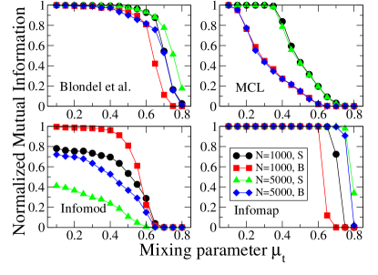
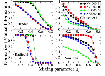
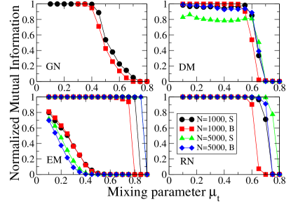
The plots of Fig. 2 illustrate the results of the analysis. The following input parameters are the same for all benchmark graphs used here, as well as in Sections VI.2, VI.3 and VI.4: the average degree is $20$, the maximum degree $50$, the exponent of the degree distribution is $-2$ and that of the community size distribution is $-1$. In each plot, except for the GN and the EM algorithms, we show four curves, corresponding to two different network sizes ($1000$ and $5000$ nodes) and, for a given size, to two different ranges for the community sizes, indicated by the letters $S$ and $B$: $S$ (stays for “small”) means that communities have between $10$ and $50$ nodes, $B$ (stays for “big”) means that communities have between $20$ and $100$ nodes. For the GN algorithm we show only the curves corresponding to the smaller network size, as it would have taken too long to accumulate enough statistics to present clean plots for networks of $5000$ nodes, due to the high computational complexity of the method. For the EM method we have plotted eight curves as for each set of benchmark graphs we have considered the two outcomes of the algorithm corrsponding to the different choices of initial conditions we have mentioned in the previous section, namely random (bottom curves) and planted partition (top curves). In this case, the difference in the performance of the algorithm in the two cases is remarkable. The fact that, by starting from the planted partition, the final likelihood is actually higher as compared with a random start, as we have seen in the previous section, confirms that the method has a great potential, if only one could find a better way to estimate the maximum likelihood than the greedy approach currently adopted. Nevertheless we remind that the EM also has the big drawback to require as input the number of groups to be found, which is usually unknown in applications.

As a general remark, we see that the LFR benchmark enables one to discriminate the performances of the algorithms much better than the GN benchmark, as expected. Modularity-based methods have a rather poor performance, which worsens for larger systems and smaller communities, due to the well known resolution limit of the measure Fortunato and Barthélemy (2007). The only exception is represented by the algorithm by Blondel et al., whose performance is very good, probably because the estimated modularity maximum is not a very good approximation of the real one, which is more likely found by simulated annealing. The Cfinder, the MCL and the method by Radicchi et al. do not have impressive performances either, and display a similar pattern, i.e. the performance is severely affected by the size of the communities (for larger communities it gets worse, whereas for small communities it is decent), whereas it looks rather insensitive to the size of the network. The DM has a fair performance, but it gets worse if the network size increases. The same trend is shown by Infomod, where the performance worsens considerably with the increase of the network size. Infomap and RN have the best performances, with the same pattern with respect to the size of the network and of the communities: up to values of $\mu_{t}\sim 1/2$ both methods are capable to derive the planted partition in the $100\%$ of cases.

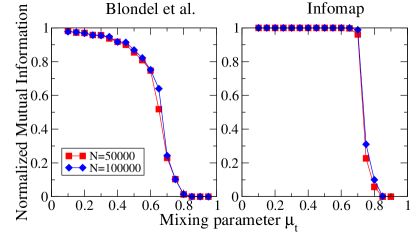
We conclude that Infomap, the RN method and the method by Blondel et al. are the best performing algorithms on the LFR undirected and unweighted benchmark. Since Infomap and the method by Blondel et al. are also very fast, essentially linear in the network size, we wonder how good their performance is on much larger graphs than those considered in Fig. 2. For this reason we carried out another set of tests of these two algorithms on the LFR benchmark, by considering graphs with $50000$ and $100000$ nodes. We have done so also because in the tests that can be found in the literature on community detection one typically uses very small graphs, and the performance can change considerably on large graphs. In Fig. 3 we show the performance of the two methods. Due to the large network size, we decided to pick a broad range of community sizes, from $20$ to $1000$ nodes. In this way, the heterogeneity of the community sizes is manifest. The maximum degree here was fixed to $200$. Remarkably, the performance of the method by Blondel et al. is worse than on the smaller graphs of Fig. 2, whereas that of Infomap is stable and does not seem to be affected.

Figure 3: Tests of the algorithm by Blondel et al. and Infomap on large LFR benchmark graphs with undirected and unweighted links.

VI.2 Directed and unweighted graphs

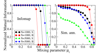
Directedness is an essential features of many real networks. Ignoring direction, as one often does or is forced to do, may reduce considerably the information that one can extract from the network structure. In particular, neglecting link directedness when looking for communities may lead to partial, or even misleading, results. In the literature there has been no benchmark for directed graphs with communities for a long time. However, we have recently extended the LFR benchmark to directed networks Lancichinetti and Fortunato (2009), so we are in the position to evaluate the performance of community detection algorithms in this case. The presence of directed links is a serious obstacle towards a generalization of an algorithm for community detection. Therefore, very few algorithms currently available are able to handle directed graphs. In the set of methods we consider here, only five can be used as well for directed networks: Clauset et al., simulated annealing for modularity, Cfinder, Infomap, EM. For some of the other algorithms one may think of possible extensions which are, at present, still missing. The EM method, in its original definition of Ref. Newman and Leicht (2007), has actually problems to deal with directed graphs Ramasco and Mungan (2008). We present here a comparison of the performances of two methods, exhaustive modularity optimization via simulated annealing and Infomap. The results are in Fig. 4. Here the topological mixing parameter $\mu_{t}$ refers to the indegree of the nodes, which are distributed according to a power law as in the original undirected benchmark, while the outdegree is kept constant for all nodes, a choice made to avoid an unnecessary proliferation of input parameters. Again, we considered two different network sizes and ranges for the community size, which are the same as those in Fig. 2. The other input parameters for the benchmark are the same that we have given in Section VI.1. As expected, modularity optimization shows the same limits that emerged in Fig. 2. On the other hand, the performance of Infomap is still very good.

Figure 4: Tests of Infomap and of the exhaustive modularity optimization via simulated annealing on the LFR benchmark with directed and unweighted links.

VI.3 Undirected and weighted graphs

In this section we focus on undirected graphs with weighted links.

Figure 5: Tests of Infomap, MCL and of the exhaustive modularity optimization via simulated annealing on the LFR benchmark with undirected and weighted links.

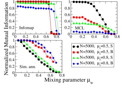
Weights are also precious sources of information Barrat et al. (2004). Just as in the case of link directedness above, neglecting weights may imply a significant limitation of the information on a graph’s properties, concealing features of real systems which may be very important and not deducible from the mere topology. Ideally, one should exploit the information from both topology and weights for a reliable analysis of a network. The LFR benchmark has been extended to weighted graphs as well Lancichinetti and Fortunato (2009). Now there are two mixing parameters, one for topology, which is the same $\mu_{t}$ we have defined and used so far, and the other for the weights, $\mu_{w}$, which is the weighted counterpart of $\mu_{t}$, i. e. it expresses the fraction of the strength of the node that lies on links connecting the node to the nodes outside its community, with respect to the total strength of the node. We remind that the strength of the node is the sum of the weights of its links. Moreover, there is an additional parameter, i. e. the exponent of the distribution for the strength: we have set it to $1.5$ for all realizations. All other parameters are the same specified in Section VI.1. Since we wish to show the results of the test on 2-dimensional plots, as we have done so far, we need to keep fixed one of the two parameters and study the dependence on the other. Here we freeze the topological mixing parameter $\mu_{t}$ and study the dependence of the results on $\mu_{w}$, so that we see how the performance of an algorithm varies when only the weights are redistributed, but the topology is fixed. The results are in Fig. 5, where we consider only three methods: Infomap, MCL and exhaustive modularity optimization via simulated annealing. The other methods have no weighted counterpart or the code for the weighted version was not available. In each plot we show four curves, corresponding to two choices for the topological mixing parameter $\mu_{t}$ and the two usual ranges of small (S) and big (B) communities that we have used so far. The network size is $5000$ nodes in each case. The Infomap by Rosvall and Bergstrom has, once more, a remarkable performance, although it worsens if communities are topologically more mixed (higher $\mu_{t}$) and larger in size (B). The MCL has a fair performance only in one case, for $\mu_{t}=0.5$ and small communities, whereas in the other extreme of big topological mixture and big communities it fails for any value of $\mu_{w}$. Modularity optimization seems to be more sensitive to the community size than to the other parameters.

VI.4 Undirected and unweighted graphs with overlapping communities

The fact that communities in real systems often overlap has attracted a lot of attention in the last years, leading to the creation of new algorithms able to deal with this special circumstance, starting from the first work by Palla et al. Palla et al. (2005). Meanwhile, a few methods have been developed Baumes et al. (2005); Zhang et al. (2007); Newman and Leicht (2007); Lancichinetti et al. (2009); Nepusz et al. (2008); Evans and Lambiotte (2009); Ahn et al. (2009); Gregory (2009), but none of them has been thoroughly tested, except on a bunch of specific networks taken from the real world. Indeed, there have been no suitable benchmark graphs with overlapping community structure, until recently Sawardecker et al. (2009); Lancichinetti and Fortunato (2009). In particular, the LFR benchmark has been extended to the case of overlapping communities Lancichinetti and Fortunato (2009), and we use it here. Of our set of algorithms, only the Cfinder is able to find overlapping communities. In principle also the EM method assigns to each node the probability that it belongs to any community, but then one would need a criterion to define which, among such probability values, is significant and shall be taken or is not significant and shall be neglected. For this reason we report the results of tests carried out with the Cfinder only.

Figure 6: Tests of the Cfinder on the LFR benchmark with undirected and unweighted links and overlapping communities. The variable on the $x$-axis is the fraction of overlapping nodes. The networks have $1000$ nodes, the other parameters are $\tau_{1}=2$, $\tau_{2}=1$, $\langle k\rangle=20$ and $k_{max}=50$.

Figure 7: Tests of the Cfinder on the LFR benchmark with undirected and unweighted links and overlapping communities. The variable on the $x$-axis is the fraction of overlapping nodes. The networks have $5000$ nodes, the other parameters are the same used for the graphs of Fig. 6.

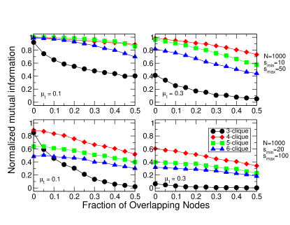
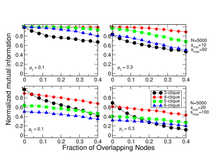
In Figs. 6 and 7 we show the results. The topological mixing parameter $\mu_{t}$ is fixed and one varies the fraction of overlapping nodes between communities. We have run the Cfinder for different types of $k$-cliques ($k$ indicates the number of nodes of the clique), with $k=3,4,5,6$. In general we notice that triangles ($k=3$) yield the worst performance, whereas $4$- and $5$-cliques give better results. In the two top diagrams community sizes range between $10$ and $50$ nodes, whereas in the bottom diagrams the range goes from $20$ to $100$ nodes. By comparing the diagrams in the top with those in the bottom we see that the algorithm performs better when communities are (on average) smaller. The networks used to produce Fig. 6 consist of $1000$ nodes, whereas those of Fig. 7 consist of $5000$ nodes. From the comparison of Fig. 6 with Fig. 7 we see that the algorithm performs better on networks of larger size.

VII Tests on random graphs

Figure 8: Tests of the algorithms on random graphs á la Erdös-Rényi (E-R) and scale free (S-F) random graphs.

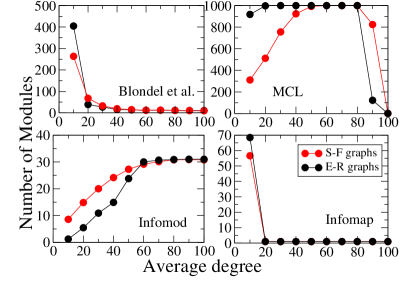
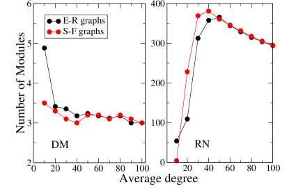
An important test of community detection algorithms, usually ignored in the literature, consists in applying them to random graphs. In random graphs, by definition, the linking probabilities of the nodes are independent of each other. In this way one does not expect that there will be inhomogeneity in the density of links on the graphs, i. e. there should be no communities. Things are not that simple, though. It is certainly true that on average this is what happens. On the other hand, specific realizations of random graphs may display pseudocommunities, i. e., clusters produced by fluctuations in the link density. This is why, for instance, the maximum modularity of partitions in random graphs is not small Guimerà et al. (2004); Reichardt and Bornholdt (2006a, b); Reichardt and Bornholdt (2007). However, a good method should distinguish between such pseudocommunities and meaningful modules. This is why we still expect to find no communities in random graphs. We considered two types of graphs: random graphs á la Erdös-Rényi Erdös and Rényi (1959), which have a binomial degree distribution, and random graphs with power law degree distributions (scale free). The latter have been built via the configuration model Molloy and Reed (1995), starting from a fixed degree sequence for the nodes obeying the predefinite power law distribution. The exponent of the distribution is $-2$, the maximum degree was fixed to $200$. The size of all graphs, Erdös-Rényi and scale free, is fixed to $1000$ nodes. In Fig. 8 we show the number of modules found by various algorithms as a function of the average degree of the graph. Each point corresponds to an average over $100$ graph realizations. We do not show the results of the EM method, because the number of modules must be given by input, and of the GN algorithm because it is too slow to be used for the analysis.

The best performance is that of the method by Radicchi et al., which always finds a single cluster comprising all nodes. Another reasonable answer is to find as many clusters as there are nodes, like the MCL. Here, however, the answer depends on the average degree $\langle k\rangle$ of the graph: if $\langle k\rangle$ is very low or very large the number of modules is smaller than $1000$, i.e. the method finds small groups of nodes. This is particularly evident for scale free graphs. Modularity-based methods, like Clauset et al., the exhaustive optimization via simulated annealing, and the algorithm by Blondel et al. are not so good, as they always find a few clusters, even in the limit of large $\langle k\rangle$: this is actually well known Reichardt and Bornholdt (2006b). This is also the case for the DM method, which performs a sort of modularity optimization, on the restricted set of partitions delivered by hierarchical clustering. Infomod and the RN method find non-trivial partitions for any value of $\langle k\rangle$. The Cfinder finds a single module for very low values of $\langle k\rangle$ and then a rapidly rising number of modules as $\langle k\rangle$ increases. Since the modules are strongly overlapping in this case, they may exceed the number of nodes, as we see from the plot. Instead, Infomap always finds a single module comprising all nodes, except when $\langle k\rangle$ is low.

VIII Summary

We have carried out a comparative analysis of the performances of algorithms for community detection on various graphs: the GN and LFR benchmarks and random graphs. Link direction, weights and the possibility for communities to overlap have been taken into account in dedicated tests. We conclude that the Infomap method by Rosvall and Bergstrom Rosvall and Bergstrom (2008) is the best performing on the set of benchmarks we have examined here. In particular, its results on the LFR benchmark graphs, which are much more difficult to examine than the GN benchmark graphs, as clearly shown by Figs. 1 and 2, are encouraging about the reliability of the method in applications to real graphs. Among the other things, the method can be applied to weighted and directed graphs as well, with excellent performances, so it has a large spectrum of potential applications. The algorithms by Blondel et al. Blondel et al. (2008) and by Ronhovde and Nussinov (RN) Ronhovde and Nussinov (2009) also look very good from our analysis and could be used as well. In fact, for a study of the community structure in real graphs, one could think of using all three methods, to be able to extract some algorithm-independent information. Furthermore, as we have seen in Section IV, these methods have a low computational complexity, so one could use them on graphs with millions of nodes and links. On the other hand, the algorithms are not able to account for overlapping communities, so they need to be properly refined to deal with this possibility, which is common in many real systems.

One may object that, despite the features planted in the LFR benchmark, i. e. the fat-tailed distributions of degree and community size, which are actually observed in real networks, our artificial graphs are still different from real systems. For instance, the clustering coefficient Watts and Strogatz (1998) of the LFR benchmark is very low, due to the very small number of triangles, whereas real networks are characterized by many triangles and consequently a high clustering coefficient. On the one hand the GN benchmark also has very few triangles and low clustering coefficient (the LFR benchmark is just a generalization of the GN benchmark), nevertheless people have used it extensively for testing algorithms. On the other hand, nothing forbids to modify the building mechanism of the LFR benchmark so that it does include triangles. This is actually a potentially interesting improvement of the benchmark, that deserves some attention in the future.

Another important remark is in order. Our whole analysis has made use of graphs with a “flat” community structure, without hierarchy. Many real networks instead have a hierarchical community structure, with communities inside other communities. Good methods must be able to understand when a network has no communities, a flat or a hierarchical community structure. For an analysis of this kind we would need hierarchical benchmarks. There is actually a hierarchical version of the GN benchmark Arenas et al. (2006), not yet one of the LFR benchmark, which is sorely needed. Methods to find communities in multipartite graphs have yet to be tested as well.

From all of the above it is clear that this manuscript does not “kill” the issue of the actual efficiency and reliability of community detection methods. Our analysis represents a first step, but it is clear that much more needs to be done along these lines.