Event-by-event simulation of quantum phenomena
Abstract
We discuss recent progress in the development of simulation algorithms that do not rely on any concept of quantum theory but are nevertheless capable of reproducing the averages computed from quantum theory through an event-by-event simulation. The simulation approach is illustrated by applications to Einstein-Podolsky-Rosen-Bohm experiments with photons.
keywords:
Quantum theory, EPR paradox, Computational techniquesPACS:
02.70.-c , 03.65.-w, , , , ,
1 Introduction
Computer simulation is widely regarded as complementary to theory and experiment [1]. The standard approach is to start from one or more basic equations of physics and to employ a numerical algorithm to solve these equations. This approach has been highly successful for a wide variety of problems in science and engineering. However, there are a number of physics problems, very fundamental ones, for which this approach fails, simply because there are no basic equations to start from.

Indeed, as is well-known from the early days in the development of quantum theory, quantum theory has nothing to say about individual events [2, 3, 4]. Reconciling the mathematical formalism that does not describe individual events with the experimental fact that each observation yields a definite outcome is referred to as the quantum measurement paradox and is the most fundamental problem in the foundation of quantum theory [3].
In view of the quantum measurement paradox, it is unlikely that we can find algorithms that simulate the experimental observation of individual events within the framework of quantum theory. Of course, we could simply use pseudo-random numbers to generate events according to the probability distribution that is obtained by solving the time-independent Schrödinger equation. However, the challenge is to find algorithms that simulate, event-by-event, the experimental observations of, for instance, interference without first solving the Schrödinger equation.
This paper is not about a new interpretation or an extension of quantum theory. The proof that there exist simulation algorithms that reproduce the results of quantum theory has no direct implications on the foundations of quantum theory: These algorithms describe the process of generating events on a level of detail about which quantum theory has nothing to say [3, 4]. The average properties of the data may be in perfect agreement with quantum theory but the algorithms that generate such data are outside of the scope of what quantum theory can describe.
In a number of recent papers [5, 6, 7, 8, 9, 10, 11, 12, 13, 14, 15, 16, 17], we have demonstrated that locally-connected networks of processing units can simulate event-by-event, the single-photon beam splitter and Mach-Zehnder interferometer experiments, universal quantum computation, real Einstein-Podolsky-Rosen-Bohm (EPRB) experiments, Wheeler’s delayed choice experiment and the double-slit experiment with photons. Our work suggests that we may have discovered a procedure to simulate quantum phenomena using event-based, particle-only processes that satisfy Einstein’s criterion of local causality, without first solving a wave equation. In this paper, we limit the discussion to event-by-event simulations of real EPRB experiments.
2 EPRB experiments
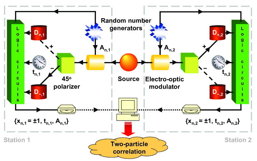
In Fig. 1, we show a schematic diagram of an EPRB experiment with photons (see also Fig. 2 in [18]). The source emits pairs of photons. Each photon of a pair propagates to an observation station in which it is manipulated and detected. The two stations are separated spatially and temporally [18]. This arrangement prevents the observation at station 1 (2) to have a causal effect on the data registered at station (1) [18]. As the photon arrives at station , it passes through an electro-optic modulator that rotates the polarization of the photon by an angle depending on the voltage applied to the modulator. These voltages are controlled by two independent binary random number generators. As the photon leaves the polarizer, it generates a signal in one of the two detectors. The station’s clock assigns a time-tag to each generated signal. Effectively, this procedure discretizes time in intervals of a width that is determined by the time-tag resolution [18]. In the experiment, the firing of a detector is regarded as an event.
As we wish to demonstrate that it is possible to reproduce the results of quantum theory (which implicitly assumes idealized conditions) for the EPRB gedanken experiment by an event-based simulation algorithm, it would be logically inconsistent to “recover” the results of the former by simulating nonideal experiments. Therefore, we consider ideal experiments only, meaning that we assume that detectors operate with 100% efficiency, clocks remain synchronized forever, the “fair sampling” assumption is satisfied [19], and so on. We assume that the two stations are separated spatially and temporally such that the manipulation and observation at station 1 (2) cannot have a causal effect on the data registered at station (1). Furthermore, to realize the EPRB gedanken experiment on the computer, we assume that the orientation of each electro-optic modulator can be changed at will, at any time. Although these conditions are very difficult to satisfy in real experiments, they are trivially realized in computer experiments.
In the experiment, the firing of a detector is regarded as an event. At the th event, the data recorded on a hard disk at station consists of , specifying which of the two detectors fired, the time tag indicating the time at which a detector fired, and the two-dimensional unit vector that represents the rotation of the polarization by the electro-optic modulator. Hence, the set of data collected at station during a run of events may be written as
| (1) |
In the (computer) experiment, the data may be analyzed long after the data has been collected [18]. Coincidences are identified by comparing the time differences with a time window [18]. Introducing the symbol to indicate that the sum has to be taken over all events that satisfy for , for each pair of directions and of the electro-optic modulators, the number of coincidences between detectors () at station 1 and detectors () at station 2 is given by
| (2) |
where is the Heaviside step function. We emphasize that we count all events that, according to the same criterion as the one employed in experiment, correspond to the detection of pairs. The average single-particle counts and the two-particle average are defined by
| (3) |
and
| (4) | |||||
respectively. In Eqs. (3) and (4), the denominator is the sum of all coincidences.
For later use, it is expedient to introduce the function
| (5) |
and its maximum
| (6) |
2.1 Analysis of real experimental data
We illustrate the procedure of data analysis and the importance of the choice of the time window by analyzing a data set (the archives Alice.zip and Bob.zip) of an EPRB experiment with photons that is publicly available [20].
In the real experiment, the number of events detected at station 1 is unlikely to be the same as the number of events detected at station 2. In fact, the data sets of Ref. [20] show that station 1 (Alice.zip) recorded 388455 events while station 2 (Bob.zip) recorded 302271 events. Furthermore, in the real EPRB experiment, there may be an unknown shift (assumed to be constant during the experiment) between the times gathered at station 1 and the times recorded at station 2. Therefore, there is some extra ambiguity in matching the data of station 1 to the data of station 2.
A simple data processing procedure that resolves this ambiguity consists of two steps [22]. First, we make a histogram of the time differences with a small but reasonable resolution (we used ns). Then, we fix the value of the time-shift by searching for the time difference for which the histogram reaches its maximum, that is we maximize the number of coincidences by a suitable choice of . For the case at hand, we find ns. Finally, we compute the coincidences, the two-particle average, and using the expressions given earlier. The average times between two detection events is ms and ms for Alice and Bob, respectively. The number of coincidences (with double counts removed) is 13975 and 2899 for ( ns, ns) and ( , ns) respectively.


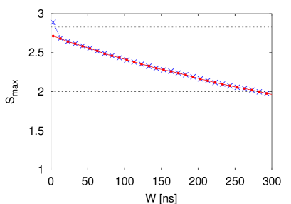
In Fig. 2 we present the results for as a function of the time window . First, it is clear that decreases significantly as increases but it is also clear that as , is not very sensitive to the choice of [22]. Second, the procedure of maximizing the coincidence count by varying reduces the maximum value of from a value 2.89 that considerably exceeds the maximum for the quantum system (, see Section 3) to a value 2.73 that violates the Bell inequality (, see Ref. [21]) and is less than the maximum for the quantum system.
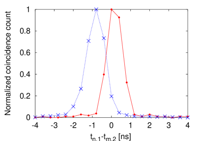
Finally, we use the experimental data to show that the time delays depend on the orientation of the polarizer. To this end, we select all coincidences between and (see Fig. 1) and make a histogram of the coincidence counts as a function of the time-tag difference, for fixed orientation and the two orientations (other combinations give similar results). The results of this analysis are shown in Fig. 3. The maximum of the distribution shifts by approximately 1 ns as the polarizer at station 2 is rotated by , a demonstration that the time-tag data is sensitive to the orientation of the polarizer at station 2. A similar distribution of time-delays (of about the same width) was also observed in a much older experimental realization of the EPRB experiment [23]. The time delays that result from differences in the orientations of the polarizers is much larger than the average time between detection events, which for the data that we analyzed is about 30000 ns. In other words, the loss in correlation that we observe as a function of increasing (see Fig. 2) cannot be explained by assuming that we calculate correlations using photons that belong to different pairs.
Strictly speaking, we cannot derive the time delay from classical electrodynamics: The concept of a photon has no place in Maxwell’s theory. A more detailed understanding of the time delay mechanism requires dedicated, single-photon retardation measurements for these specific optical elements.
2.2 Role of the coincidence window
The crucial point is that in any real EPR-type experiment, it is necessary to have an operational procedure to decide if the two detection events correspond to the observation of one two-particle system or to the observation of two single-particle systems. In standard “hidden variable” treatments of the EPR gedanken experiment [21], the operational definition of “observation of a single two-particle system” is missing. In EPRB-type experiments, this decision is taken on the basis of coincidence in time [23, 25, 18].
Our analysis of the experimental data shows beyond doubt that a model which aims to describe real EPRB experiments should include the time window and that the interesting regime is , not as is assumed in all textbook treatments of the EPRB experiment. Indeed, in quantum mechanics textbooks it is standard to assume that an EPRB experiment measures the correlation [21]
| (7) |
which we obtain from Eq. (2) by taking the limit . Although this limit defines a valid theoretical model, there is no reason why this model should have any bearing on the real experiments, in particular because experiments pay considerable attention to the choice of . In experiments a lot of effort is made to reduce (not increase) [18, 22].
3 Quantum theory
According to the axioms of quantum theory [4], repeated measurements on the two-spin system described by the density matrix yield statistical estimates for the single-spin expectation values
| (8) |
and the two-spin expectation value
| (9) |
where are the Pauli spin-1/2 matrices describing the spin of particle [4], and and are unit vectors. We have introduced the tilde to distinguish the quantum theoretical results from the results obtained from the data sets .
The quantum theoretical description of the EPRB experiment assumes that the system is represented by the singlet state of two spin-1/2 particles, where and denote the horizontal and vertical polarization and the subscripts refer to photon 1 and 2, respectively. For the singlet state , and
| (10) |
4 Simulation model
A concrete simulation model of the EPRB experiment sketched in Fig. 1 requires a specification of the information carried by the particles, of the algorithm that simulates the source and the observation stations, and of the procedure to analyze the data. In the following, we describe a slightly modified version of the algorithm proposed in Ref. [9], tailored to the case of photon polarization.
Source and particles: The source emits particles that carry a vector , representing the polarization of the photons that travel to station and station , respectively. Note that , indicating that the two particles have orthogonal polarizations. The “polarization state” of a particle is completely characterized by , which is distributed uniformly over the whole interval . For the purpose of mimicing the apparent unpredictability of the experimental data, we use uniform random numbers. However, from the description of the algorithm, it will be clear that the use of random numbers is not essential. Simple counters that sample the intervals in a systematic, but uniform, manner might be employed as well.
Observation station: The electro-optic modulator in station rotates by an angle , that is . The number of different rotation angles is chosen prior to the data collection (in the experiment of Weihs et al., [18]). We use random numbers to fill the arrays and . During the measurement process we use two uniform random numbers to select the rotation angles and . The electro-optic modulator then rotates by , yielding .
The polarizer at station projects the rotated vector onto its -axis: , where denotes the unit vector along the -axis of the polarizer. For the polarizing beam splitter, we consider a simple model: If the particle causes to fire, otherwise fires. Thus, the detection of the particles generates the data .
Time-tag model: To assign a time-tag to each event, we assume that as a particle passes through the detection system, it may experience a time delay. In our model, the time delay for a particle is assumed to be distributed uniformly over the interval , an assumption that is not in conflict with available data [22]. In practice, we use uniform random numbers to generate . As in the case of the angles , the random choice of is merely convenient, not essential. From Eq. (2), it follows that only differences of time delays matter. Hence, we may put . The time-tag for the event is then .
There are not many options to make a reasonable choice for . Assuming that the particle “knows” its own direction and that of the polarizer only, we can construct one number that depends on the relative angle: . Thus, depends on only. Furthermore, consistency with classical electrodynamics requires that functions that depend on the polarization have period [24]. Thus, we must have . We already used to determine whether the particle generates a or signal. By trial and error, we found that yields useful results [9, 10, 11, 12, 13]. Here, is the maximum time delay and defines the unit of time, used in the simulation and is a free parameter of the model. In our numerical work, we set .
Data analysis: For fixed and , the algorithm generates the data sets just as experiment does [18]. In order to count the coincidences, we choose a time-tag resolution and a coincidence window . We set the correlation counts to zero for all and . We compute the discretized time tags for all events in both data sets. Here denotes the smallest integer that is larger or equal to , that is . According to the procedure adopted in the experiment [18], an entangled photon pair is observed if and only if . Thus, if , we increment the count .

5 Simulation results
The simulation proceeds in the same way as the experiment, that is we first collect the data sets , and then compute the coincidences Eq. (2) and the correlation Eq. (4). The simulation results for the coincidences depend on the time-tag resolution , the time window and the number of events , just as in real experiments [18].
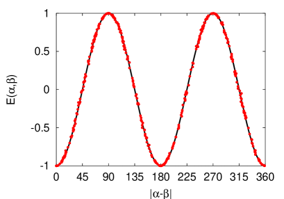
Figure 4 shows simulation data for as obtained for d=2, and . In the simulation, for each event, the random numbers select one pair out of , where the angles and are fixed before the data is recorded. The data shown has been obtained by allowing for different angles per station. Hence, forty random numbers from the interval [0,360[ were used to fill the arrays and . For each of the events, two different random number generators were used to select the angles and . The statistical correlation between and was measured to be less than .
From Fig. 4, it is clear that the simulation data for are in excellent agreement with quantum theory. Within the statistical noise, the simulation data (not shown) for the single-spin expectation values also reproduce the results of quantum theory.
Additional simulation results (not shown) demonstrate that the kind of models described earlier are capable of reproducing all the results of quantum theory for a system of two S=1/2 particles [9, 10, 11, 12, 13]. Furthermore, to first order in and in the limit that the number of events goes to infinity, one can prove rigorously that these simulation models give the same expressions for the single- and two-particle averages as those obtained from quantum theory [9, 10, 11, 12, 13].
6 Discussion
Starting from the factual observation that experimental realizations of the EPRB experiment produce the data (see Eq. (1)) and that coincidence in time is a key ingredient for the data analysis, we have described a computer simulation model that satisfies Einstein’s criterion of local causality and, exactly reproduces the correlation that is characteristic for a quantum system in the singlet state.
We have shown that whether or not these simulation models produce quantum correlations depends on the data analysis procedure that is performed (long) after the data has been collected: In order to observe the correlations of the singlet state, the resolution of the devices that generate the time-tags and the time window should be made as small as possible. Disregarding the time-tag data ( or ) yields results that disagree with quantum theory but agree with the models considered by Bell [21]. Our analysis of real experimental data and our simulation results show that increasing the time window changes the nature of the two-particle correlations [9, 10, 11, 12, 13].
According to the folklore about Bell’s theorem, a procedure such as the one that we described should not exist. Bell’s theorem states that any local, hidden variable model will produce results that are in conflict with the quantum theory of a system of two particles [21]. However, it is often overlooked that this statement can be proven for a (very) restricted class of probabilistic models only. In fact, Bell’s theorem does not necessarily apply to the systems that we are interested in as both simulation algorithms and actual data do not need to satisfy the (hidden) conditions under which Bell’s theorem hold [26, 27, 28, 29].
Furthermore, the apparent conflict between the fact that there exist event-based simulation models that satisfy Einstein’s criterion of local causality and reproduce all the results of the quantum theory of a system of two particles and the folklore about Bell’s theorem, stating that such models are not supposed to exist dissolves immediately if one recognizes that Bell’s extension of Einstein’s concept of locality to the domain of probabilistic theories relies on the hidden, fundamental assumption that the absence of a causal influence implies logical independence [30, 31].
The simulation model that is described in this paper is an example of a purely ontological model that reproduces quantum phenomena without first solving the quantum problem. The salient features of our simulation models [5, 6, 7, 8, 9, 10, 11, 14] are that they
-
1.
generate, event-by-event, the same type of data as recorded in experiment,
-
2.
analyze data according to the procedure used in experiment,
-
3.
satisfy Einstein’s criterion of local causality,
-
4.
do not rely on any concept of quantum theory or probability theory,
-
5.
reproduce the averages that we compute from quantum theory.
Acknowledgments
We thank K. De Raedt and A. Keimpema for many useful suggestions and extensive discussions.
References
- [1] D. P. Landau, K. Binder, A Guide to Monte Carlo Simulation in Statistical Physics, Cambridge University Press, Cambridge, 2000.
- [2] D. Bohm, Quantum Theory, Prentice-Hall, New York, 1951.
- [3] D. Home, Conceptual Foundations of Quantum Physics, Plenum Press, New York, 1997.
- [4] L. E. Ballentine, Quantum Mechanics: A Modern Development, World Scientific, Singapore, 2003.
- [5] K. De Raedt, H. De Raedt, K. Michielsen, Comp. Phys. Comm. 171 (2005) 19.
- [6] H. De Raedt, K. De Raedt, K. Michielsen, J. Phys. Soc. Jpn. Suppl. 76 (2005) 16.
- [7] H. De Raedt, K. De Raedt, K. Michielsen, Europhys. Lett. 69 (2005) 861.
- [8] K. Michielsen, K. De Raedt, H. De Raedt, J. Comput. Theor. Nanosci. 2 (2005) 227.
- [9] K. De Raedt, K. Keimpema, H. De Raedt, K. Michielsen, S. Miyashita, Euro. Phys. J. B 53 (2006) 139.
- [10] H. De Raedt, K. De Raedt, K. Michielsen, K. Keimpema, S. Miyashita, J. Phys. Soc. Jpn. 76 (2007) 104005.
- [11] K. De Raedt, H. De Raedt, K. Michielsen, Comp. Phys. Comm. 176 (2007) 642.
- [12] H. De Raedt, K. De Raedt, K. Michielsen, K. Keimpema, S. Miyashita, J. Comp. Theor. Nanosci. 4 (2007) 957.
- [13] H. De Raedt, K. Michielsen, S. Miyashita, K. Keimpema, Euro. Phys. J. B 58 (2007) 55.
- [14] S. Zhao, H. De Raedt, J. Comp. Theor. Nanosci. 5 (2008) 490.
- [15] S. Zhao, H. De Raedt, K. Michielsen, Found. of Phys. 38 (2008) 322.
- [16] S. Zhao, S. Yuan, H. De Raedt, K. Michielsen, Europhys. Lett. 82 (2008) 40004.
- [17] F. Jin, S. Yuan, H. D. Raedt, K. Michielsen, arXiv:0809.0616.
- [18] G. Weihs, T. Jennewein, C. Simon, H. Weinfurther, A. Zeilinger, Phys. Rev. Lett. 81 (1998) 5039.
- [19] G. Adenier, A. Y. Khrennikov, J. Phys. B: At. Mol. Opt. Phys. 40 (2007) 131.
- [20] http://www.quantum.at/research/photonentangle/ bellexp/data.html. The results presented here have been obtained by assuming that the data sets *_V.DAT contain IEEE-8 byte (instead of 8-bit) double-precision numbers and that the least significant bit in *_C.DAT specifies the position of the switch instead of the detector that fired.
- [21] J. S. Bell, Speakable and unspeakable in quantum mechanics, Cambridge University Press, Cambridge, 1993.
- [22] G. Weihs, Ein Experiment zum Test der Bellschen Ungleichung unter Einsteinscher Lokalität, Ph.D. thesis, University of Vienna, http://www.quantum.univie.ac.at/publications/ thesis/gwdiss.pdf (2000).
- [23] C. A. Kocher, E. D. Commins, Phys. Rev. Lett. 18 (1967) 575.
- [24] M. Born, E. Wolf, Principles of Optics, Pergamon, Oxford, 1964.
- [25] J. F. Clauser, M. A. Horne, Phys. Rev. D 10 (1974) 526.
- [26] L. Sica, Opt. Comm. 170 (1999) 55.
- [27] K. Hess, W. Philipp, Proc. Natl. Acad. Sci. USA 101 (2004) 1799.
- [28] K. Hess, W. Philipp, Found. of Phys. 35 (2005) 1749.
- [29] T.M. Nieuwenhuizen, in Foundations of Probability and Physics - 5, vol. 1101, ed. by L. Accardi, G. Adenier, C. Fuchs, G. Jaeger, A. Khrennikov, J.A. Larsson, S. Stenholm (AIP Conference Proceedings, Melville and New York, 2009), vol. 1101, p. 127.
- [30] A. Fine, Synthese 29 (1974) 257.
- [31] E. T. Jaynes, Clearing up mysteries - The original goal, in: J. Skilling (Ed.), Maximum Entropy and Bayesian Methods, Vol. 36, Kluwer Academic Publishers, Dordrecht, 1989, p. 1.