Subspace modelling for structured noise suppression
Abstract
The problem of structured noise suppression is addressed by i)modelling the subspaces hosting the components of the signal conveying the information and ii)applying a non-extensive nonlinear technique for effecting the right separation. Although the approach is applicable to all situations satisfying the hypothesis of the proposed framework, this work is motivated by a particular scenario, namely, the cancellation of low frequency noise in broadband seismic signals.
1 Introduction
The problem of structured noise suppression concerns the elimination of signal components produced by phenomena interfering with the observations of interest. This problem can be addressed by linear techniques provided that the subspaces hosting the signal components are complementary and well separated [1, 2, 3, 4]. More precisely, if a signal represented by the ket is produced as the superposition of two components and , provided that , the components of the superposition can be separated by an oblique projection. Even when this condition is theoretically fulfilled, if the subspaces and are not well separated, the concomitant linear problem for extracting one of the signal components may be ill posed, which causes the failure to correctly split the signal by a linear operation. Hence, nonlinear techniques for determining a subspace , such that , and the projection onto along is well posed, have been considered [3, 4, 5]. In those publications the theoretically complementary subspaces and are assumed to be known. Nevertheless, the condition is strong and the possibility of meeting it depends on the ability to generate the right model for the subspaces. Unfortunately, the modelling of the complementary subspaces by pure physical considerations is not always possible and one needs to relay on more general mathematical modelling.
Although the technique for subspace modelling we introduce here is applicable to different situations, the work is motivated by a particular problem relevant to the processing of seismic signals. In the nearshore these signals may be affected by a population of low-frequency waves called infragravity waves[6]. This type of noise may be also unavoidable in bottom broadband seismic observations [7]. The interested reader is refereed to [8] for explanations on how infragravity waves are generated. We restrict our consideration to the problem of reducing that type of structured low frequency noise from broadband seismic signals.
Our purpose is twofold. We aim at i)mathematically modelling the subspaces to represent the signal components ii)provide a sparse enough representation of the signals so as to make sure that the correct splitting can be realized.
Under the hypothesis that one of the signals components lies in the subspace of low frequency signals, we determine the subspace of the other component in an adaptive manner. We assume that such a component belongs to an unknown spline space and determine the knots characterizing the space by taking into account the curvature points of the signal in hand. In that sense, the space is ‘adapted’ to the particular signal being analyzed. In line with [4] we tackle the problem of finding the representation of this component through the minimization of the -norm like quantity, which is closely related to the non-extensive entropy introduced as ingredient of a thermodynamic framework in the seminal paper by Tsallis [9] and ever since broadly applied in physics [9, 10, 11, 12, 13, 14, 15, 16] and other disciplines [17].
The paper is organized as follows: In Section 2 we address the problem of subspaces modelling and discuss the non-extensive nonlinear technique yielding the right signal splinting. A numerical simulation concerning the filtering of low frequency noise from a seismic signal is presented in Section 3. The conclusions are drawn in Section 4.
2 Adaptive subspace modelling for structured noise filtering
As already mentioned, we are concerned with the problem of separating from a signal those components which are not relevant to the phenomenon of interest. For simplicity we consider that a signal is the superposition of only two components and the goal is to find a suitable model for the subspaces hosting such component. Since out work is motivated by the specific problem of filtering low frequency noise from a seismic signal, we further assume that the subspace representing that type of structured noise is spanned by a few Fourier functions. In accordance with previous works we denote such a subspace as and consider it to be fixed. The composed signal is the superposition with . The goal is to model the subspace fulfilling the theoretical condition , regardless of the fact that the two subspaces may be too close to each other for the signal separation to be obtained via a linear approach. We allow for this difficulty by introducing the additional hypothesis that is well represented in a subspace of , which is tantamount to assuming that has a ‘sparse enough’ representation in . We further assume that is well approximated in a dedicated spline space to be constructed as described in the next section.
2.1 Finding the appropriate spline space
Let us start by stating the few definitions on spline spaces which are needed for setting up our mathematical framework. For a complete treatment of splines we refer to the fundamental books [18, 19, 20].
Definition 1.
Given a finite closed interval we define a partition of as the finite set of points
| (1) |
We further define subintervals as: and .
Definition 2.
Let be the space of polynomials of degree smaller or equal to . Let be a positive integer and define
| (2) |
where indicates the restriction of the function on the interval .
An extended partition with single inner knots associated with is a set such that
and the first and last points can be arbitrarily chosen. With each fixed extended partition there is associated a unique B-spline basis for , that we denote as . The B-spline can be defined by the recursive formulae [18]:
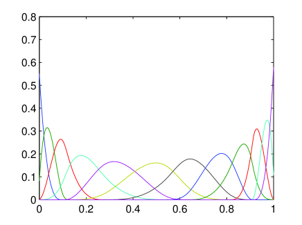
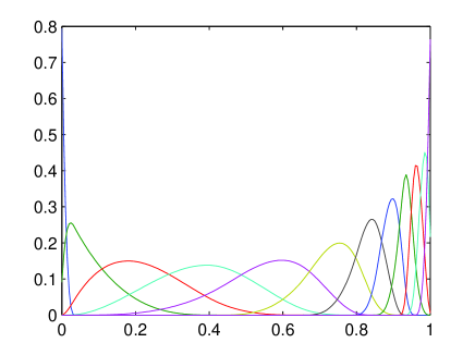
For each order, , the corresponding spline space is determined by the number and position of the knots. In Fig 1 we show B-spline basis for two different cubic spline spaces () having the same number of knots but located at different positions.
In order to find the appropriate partition giving rise to the appropriate spline space to represent a given signal , we first determine the critical points of the signal’s curvature, i.e., we find the set defined as
| (3) |
The entries in are chosen as the initial knots of . Extra knots are obtained by subdivisions between consecutive knots in so as to generate a partition with the desired number of knots. An algorithm for implementing this procedure on a signal given as a discrete piece of data is outlined in [21]. We would like to be able to use this procedure on the signal we need to represent, namely the component , but, of course we do not have access to this signal; our goal is to find it!. Thus, in line with [3, 4] we proceed as explained below.
Since in our framework is fixed and known, we can construct the orthogonal projector onto that we denote . Assuming now that , for some order and some partition , we can use B-splines to span the space so that for we have
| (4) |
Hence, by applying the projector on both sides of (4) we further have
| (5) |
Denoting by the identity operator in , the projector is obtainable from the relation . Therefore the component is available and can be used to determine the knots of the spline space to represent it.
Let us suppose then that through the curvature function (3) we obtain a suitable partition for the space to represent . Now, in order to obtain the component from in the most usual case involving subspaces and close to each other, we need to find the representation of in a subspace of . The approach for achieving such an aim is discussed in the next section.
2.2 Determination of the signal representation through a nonlinear non-extensive approach
At this point we can assume that we know the spanning set for so that henceforth the problem is reduced to finding the representation (5) with sparse coefficients. For this we could apply the approach proposed in [4], which entails to use the normal equations
| (6) |
as constraints for the minimization of the norm like quantity but incorporating the equations in a stepwise manner. However, in the case motivating this work the number of necessary constraints is large enough to make the whole process slow. Hence rather than using the approach proposed in [4] we take an alternative route and apply a regularized version of the FOCUSS algorithm, which implies to minimize the functional
where is a regularization parameter. The algorithm for implementing the approach is based on re-weighted least squares and is given in [22]. It comprises the following simple steps
-
1)
For each fixed set a value for and a value for the initial vector .
-
2)
At each iteration, say iteration , define the operators
where the representation of the kets are B-spline functions of order .
-
3)
Compute as
where indicates the adjoint of and the identity operator.
-
4)
Given a small , while , repeat 2) and 3)
For the derivation of the method and discussion on convergence issues see [22].
When the numerical convergence has been reached, say at iteration , set and compute the required component as
3 Application to filtering of structured low frequency noise from a seismic signal
We apply here the proposed approach to filtering low frequency noise from a seismic signal. As already mentioned, a common interference with broadband seismic signals is produced by long waves, generated by known or unknown sources, called infragravity waves [6]. This interference is referred to as low frequency noise as it falls in a frequency range of up to 0.05 Hz. Thus, the model for the subspace of that type of structured noise, on a signal given by samples, is
| (7) |
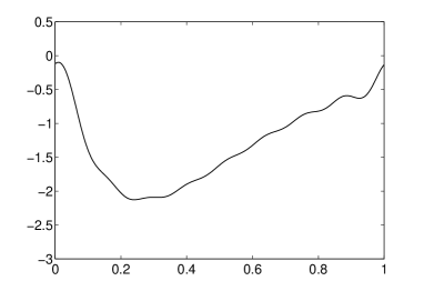
The particular realization of the noise we have simulated is plotted in the top left graph of Fig 2 (signal ). However, it is appropriate to recall that the success of the approach does not depends on the actual form of the noise (as long as it belongs to the subspace given in (7)) because the approach guarantees the suppression of the whole subspace .
The seismic signal shown in the right graph of Fig 2 is a piece of a test signal distributed by the seismic industry. The left bottom graph is the superposition of the signals in the top graphs, i.e. We fist subtract from the component in to obtain and use this signal to find the points in the set (3). Then we subdivide uniformly those points to obtain nonuniform knots defining the signal space. Using these knots we construct the nonuniform B-spline basis for the space (MATLAB codes for the implementation of both steps are available from [23]).
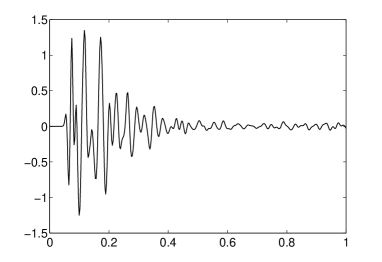
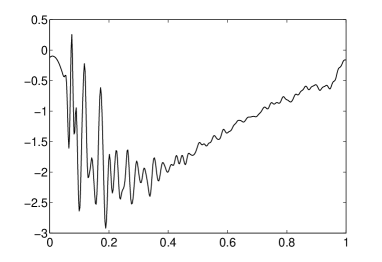
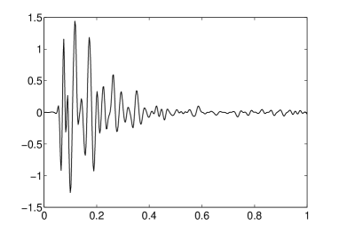
The methodology discussed in the previous section requires to fix the values for and . To allow for good resolution the regularization parameter is given a small value . As for the parameter we have let it vary in the interval with step and the best value resulted to be . The right bottom graph of Fig 2 depicts the filtered signal arising by applying the regularized FOCUSS method for and .
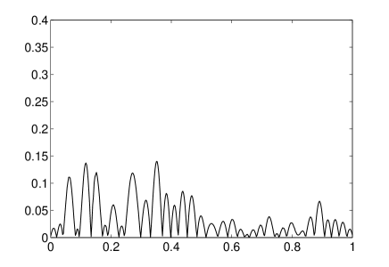
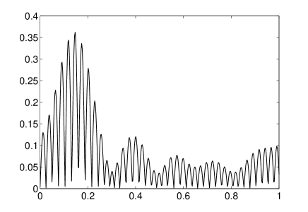
The left graph of Fig 3 plots, , the absolute value of the difference between the approximation (for ) and the true signal . For the sake of comparison, in the right graph we have plotted , where is the approximation arising by filtering with Fast Fourier Transform (FFT). For this approximation we simply take the FFT of , eliminate the frequencies components in (7), and apply the inverse transform to obtain . The comparison shows the superiority of the proposed approach with respect to standard FFT filtering.
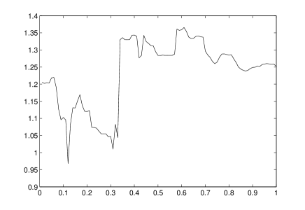
In order to analyze the dependence of the solution on the parameter we calculated the error’s norm . The plot of this error, against , is depicted in Fig 4. While there is clearly an optimum value of , the one we have used in this example (and a second best value ) it should be mentioned that for all the values of in the approximation is superior than that obtained by filtering with FFT.
4 Conclusions
The problem of structured noise suppression has been considered by modelling the subspaces of the signal components and applying a nonextensive nonlinear technique for separating them. The work was motivated by the problem of filtering infragravity waves from broadband seismic signals. For this, the noise subspace was modelled using low frequency Fourier functions and that of the other component by a dedicated spline space (adapted to the signal in hand). A simulation involving a piece of seismic signal distributed by the seismic industry and noise up to 0.05Hz has produced encouraging results in comparison with those arising by standard Fourier Transform filtering.
Acknowledgements
Support from the Engineering and Physical Sciences Research Council (EPSRC), UK, grant EPD062631, is acknowledged.
References
- [1] R. Behrens, L. Scharf, Signal processing applications of oblique projection operators, IEEE Transactions on Signal Processing 42 (1994) 1413–1424.
- [2] L. Rebollo-Neira, Constructive updating/downdating of oblique projectors: a generalization of the Gram–Schmidt process, Journal of Physics A: Mathematical and Theoretical 40 (2007) 6381–6394.
- [3] L. Rebollo-Neira, Measurements design and phenomena discrimination, J. Phys. A: Math. Theor. 42 (2009) 165210.
- [4] L. Rebollo-Neira, A. Plastino, Nonlinear non-extensive approach for identification of structured information, Phyica A, in press (2009)
- [5] L. Rebollo-Neira, Oblique matching pursuit, IEEE Signal Processing Letters 14 (10) (2007) 703–706.
- [6] R. D. Kosʹi︠a︡n, N. V. B. Pykhov, B. L. Edge, Coastal processes in tideless seas, ASCE Publications, 2000.
- [7] D. Dolenc, B. Romanowicz, B. Uhrhammer, P. McGill, D. Neuhauser, D. Stakes, Identifying and removing noise from the Monterey ocean bottom broadband seismic station (MOBB) data, Geochem. Geophys. Geosyst., 8, (2007) Q02005, doi:10.1029/2006GC001403.
- [8] W. C. Crawford, S. C. Webb, Identifying and removing tilt noise from low-frequency ( Hz) seafloor vertical seismic data, Bull. Seism. Soc. Am., 90, 952-963, 2000.
- [9] C. Tsallis, Possible generalization of Boltzmann-Gibbs statistics, J. Stat. Phys., 52, (1988) 479.
- [10] C. Tsallis Introduction to nonextensive statistical mechanics, Springer-Verlag, NY, (2009).
- [11] A. R. Plastino, A. Plastino, Tsallis Stellar Polytropes and Tsallis’ entropy, Physics Letters A, 174 (1993) 834–386.
- [12] A. R. Plastino, A. Plastino, Tsallis Entropy, Erhenfest Theorem and Information Theory, Physics Letters A, 177 (1993) 177–179.
- [13] S. Abe, Y. Okamoto, Nonextensive Statistical Mechanics and Its Applications Series: Lecture Notes in Physics , Vol. 560 Springer-Verlag, NY (2001).
- [14] A, Taruya, M. Sakagami, Gravothermal catastrophe and Tsallis’ generalized entropy of self-gravitating systems, Physica A, 307, 1-2 (2002) 185–206. AS01
- [15] J. Andrade Jr., M.P. Almeida, A.A. Moreira, G.A. Farias, Extended phase-space dynamics for the generalized nonextensive thermostatistics, Phys. Rev. E 65, (2002) 036121
- [16] G. Adesso, A. Serafini, F. Illuminati, Extremal entanglement and mixedness in continuously variable systems, Phys. Rev. A 70 (2004) 022318. ‘
- [17] M. Gell-Mann, C. Tsallis, (Editors) Nonextensive entropy Interdisciplinary Application (Santa Fe Institute Studies on the Sciences of Complexity) Oxford University Press, USA (2004).
- [18] L. Schumaker, Spline Functions: Basic Theory, Wiley, New York, 1981.
- [19] C. K. Chui, Multivariate splines, SIAM, Philadelphia, 1988.
- [20] Carl De Boor, A Practical Guide to Splines, Springer, New York, 2001.
- [21] L. Rebollo-Neira, Z. Xu, Adaptive non-uniform B-spline dictionaries on a compact interval, arXiv:0908.0691v1 [math.FA]
- [22] B.D. Rao, K. Engan, S. F. Cotter, J. Palmer, K. Kreutz-Delgado, Subset selection in noise based on diversity measure minimization, IEEE Transactions on Signal Processing, 51, 3 (2003) 760– 770, 10.1109/TSP.2002.808076.
- [23] http://www.ncrg.aston.ac.uk/Projects/HNLApprox/sigrep2.html