Model independent constraints on mass-varying neutrino scenarios
Abstract
Models of dark energy in which neutrinos interact with the scalar field supposed to be responsible for the acceleration of the universe usually imply a variation of the neutrino masses on cosmological time scales. In this work we propose a parameterization for the neutrino mass variation that captures the essentials of those scenarios and allows to constrain them in a model independent way, that is, without resorting to any particular scalar field model. Using WMAP 5yr data combined with the matter power spectrum of SDSS and 2dFGRS, the limit on the present value of the neutrino mass is eV at C.L. for the case in which the neutrino mass was lighter (heavier) in the past, a result competitive with the ones imposed for standard (i.e., constant mass) neutrinos. Moreover, for the ratio of the mass variation of the neutrino mass over the current mass we found that at C.L. for , totally consistent with no mass variation. These stringent bounds on the mass variation are not related to the neutrino free-streaming history which may affect the matter power spectrum on small scales. On the contrary, they are imposed by the fact that any significant transfer of energy between the neutrino and dark energy components would lead to an instability contradicting CMB and large scale structure data on the largest observable scales.
pacs:
14.60.St, 98.80.-k, 98.80.Cq, 98.80.EsI Introduction
Since the accelerated expansion of the universe was first observed with Type Ia supernovae (SN) Riess:1998cb ; Perlmutter:1998np , the case for a cosmological constant-like fluid that dominates the energy density of the universe has become stronger and is well established by now with the new pieces of data gathered Frieman:2008sn .
Several candidates for the accelerating component of the universe, generically dubbed dark energy (DE), have been proposed Frieman:2008sn ; DEreview1 ; DEreview2 ; Caldwell:2009ix , but understanding them theoretically and observationally has proven to be challenging. On the theoretical side, explaining the small value of the observed dark energy density component, eV, as well as the fact that both dark energy and matter densities contribute significantly to the energy budget of the present universe requires in general a strong fine tuning on the overall scale of the dark energy models. In the case in which the dark energy is assumed to be a scalar field slowly rolling down its flat potential , the so-called quintessence models Caldwell:1997ii , the effective mass of the field has to be taken of the order eV for fields with vacuum expectation values of the order of the Planck mass.
On the observational side, choosing among the dark energy models is a complicated task Linder:2008pp . Most of them can mimic a cosmological constant at late times (that is, an equation of state ) Albrecht:2006um , and all data until now are perfectly consistent with this limit. In this sense, looking for different imprints that could favor the existence of a particular model of dark energy is a path worth taking.
Our goal in this paper consists in understanding whether the so-called Mass-Varying Neutrinos (MaVaNs) scenario Gu2003 ; Fardon:2003eh ; Peccei:2004sz ; Amendola:2007yx ; Wetterich:2007kr could be constrained not only via the dark energy effects, but also by indirect signs of the neutrino mass variation during cosmological evolution, since neutrinos play a key role in several epochs Hannestad:2006zg ; Lesgourgues:2006nd . An indication of the variation of the neutrino mass would certainly tend to favor this models (at least on a theoretical basis) with respect to most DE models. One should keep in mind that MaVaNs scenarios can suffer from stability issues for the neutrino perturbations Afshordi:2005ym , although there is a wide class of models and couplings that avoid this problem Bjaelde:2007ki ; Bean:2007nx ; Bean:2007ny ; Bean:2008ac ; Bernardini:2008pn .
Similar analyses have been made in the past, but they have either assumed particular models for the interaction between the neutrinos and the DE field Brookfield:2005td ; Brookfield:2005bz ; Ichiki:2007ng , or chosen a parameterization that does not reflect the richness of the possible behavior of the neutrino mass variations Zhao:2006zf .
In order to be able to deal with a large number of models, instead of focusing on a particular model for the coupling between the DE field and the neutrino sector, we choose to parameterize the neutrino mass variation to place general and robust constraints on the MaVaNs scenario. In this sense, our work complements previous analyses by assuming a realistic and generic parameterization for the neutrino mass, designed in such a way to probe almost all the different regimes and models within the same framework. In particular, our parameterization allows for fast and slow mass transitions between two values of the neutrino mass, and it takes into account that the neutrino mass variation should start when the coupled neutrinos change their behavior from relativistic to nonrelativistic species. We can mimic different neutrino-dark energy couplings and allow for almost any monotonic behavior in the neutrino mass, placing reliable constraints on this scenario in a model independent way.
Our work is organized as follows: in Section II we give a brief review of the MaVaNs scenario and its main equations. In Section III we present our parameterization with the results for the background and the perturbation equations obtained within this context. The results of our comparison of the numerical results with the data and the discussion of its main implications are shown in section IV. Finally, in section V the main conclusions and possible future directions are discussed.
II Mass-varying neutrinos
In what follows, we consider a homogeneous and isotropic universe with a Robertson-Walker flat metric, , where is the conformal time, that can be written in terms of the cosmic time and scale factor as , in natural units (). In this case, the Friedmann equations read
| (1) | |||||
| (2) |
where the dot denotes a derivative with respect to conformal time, and the reduced Planck mass is GeV. As usual, and correspond to the total energy density and pressure of the cosmic fluid, respectively. The neutrino mass in the models we are interested in is a function of the scalar field that plays the role of the dark energy, and can be written as
| (3) |
where is a constant and different models are represented by distinct .
The fluid equation of the neutrino species can be directly obtained from the Boltzmann equation for its distribution function Brookfield:2005bz ,
| (4) |
where takes into account the variation of the neutrino mass, and is the equation of state of the species . For completeness and later use, we will define , the standard density parameter, where the current critical density is given by eV4 and km s-1 Mpc-1 is the Hubble constant.
Since the total energy momentum tensor is conserved, the dark energy fluid equation also presents an extra right-hand side term proportional to the neutrino energy momentum tensor trace, , and can be written as
| (5) |
For a homogeneous and isotropic scalar field, the energy density and pressure are given by
| (6) |
and both equations lead to the standard cosmological Klein-Gordon equation for an interacting scalar field, namely,
| (7) |
From the above equations one sees that, given a potential for the scalar field and a field-dependent mass term for the neutrino mass, the coupled system given by equations (1), (4), and (7), together with the fluid equations for the baryonic matter, cold dark matter and radiation (photons and other massless species) can be numerically solved Brookfield:2005bz . Notice that a similar approach has been used for a possible variation of the dark matter mass carroll97 and its possible interaction with the dark energy amendola00 ; amendola01 , with several interesting phenomenological ramifications farrar04 ; prd04 ; huey04 ; das05 ; Quartin:2008px ; LaVacca2009 .
Following prd04 ; das05 , equations (4) and (5) can be rewritten in the standard form,
if one defines the effective equation of state of neutrinos and DE as
The effective equation of state can be understood in terms of the dilution of the energy density of the species. In the standard noncoupled case, the energy density of a fluid with a given constant equation of state scales as . However, in the case of interacting fluids, one should also take into account the energy transfer between them, and the energy density in this case will be given by
| (10) |
where the index 0 denotes the current value of a parameter, and the redshift is defined by the expansion of the scale factor, (in the rest of this work we will assume ). For a constant effective equation of state one obtains the standard result, , as expected.
Notice that this mismatch between the effective and standard DE equations of state could be responsible for the “phantom behavior” suggested by supernovae data when fitting it using a cosmological model with noninteracting components das05 . This effect could be observable if dark energy was coupled to the dominant dark matter component. For the models discussed here, however, it cannot be significant: the neutrino fraction today () is too small to induce an “effective phantom-like” behavior.
As we commented before, the analysis until now dealt mainly with particular models, that is, with particular functional forms of the dark energy potential and field dependence of the neutrino mass . A noticeable exception is the analysis of Ref. Zhao:2006zf , in which the authors use a parameterization for the neutrino mass a là Chevallier-Polarski-Linder (CPL) Albrecht:2006um ; Chevallier:2000qy ; Linder:2002et : . However, although the CPL parameterization works well for the dark energy equation of state, it cannot reproduce the main features of the mass variation in the case of variable mass particle models. In the case of the models discussed here, for instance, the mass variation is related to the relativistic/nonrelativistic nature of the coupled neutrino species. With a CPL mass parameterization, the transition from to always takes place around , which is in fact only compatible with masses as small as eV. Hence, the CPL mass parameterization is not suited for a self-consistent exploration of all interesting possibilites.
One of the goals in this paper is to propose and test a parameterization that allows for a realistic simulation of mass-varying scenarios in a model independent way, with the minimum possible number of parameters, as explained in the next section.
III Model independent approach
III.1 Background equations
As usual, the neutrino energy density and pressure are given in terms of the zero order Fermi-Dirac distribution function by
| (11) |
where denotes the modulus of the comoving momentum (), corresponds to the number of neutrino degrees of freedom, and is the present neutrino background temperature. Notice that in the neutrino distribution function we have used the fact that the neutrinos decouple very early in the history of the universe while they are relativistic, and therefore their equilibrium distribution depends on the comoving momentum, but not on the mass Lesgourgues:2006nd . In what follows we have neglected the small spectral distortions arising from non-instantaneous neutrino decoupling Mangano:2005cc . Thus, the neutrino energy density and pressure are given by
| (12) |
| (13) |
where (assuming that depends only on the scale factor). Taking the time-derivative of the energy density, one can then obtain the fluid equation for the neutrinos,
| (14) |
where is the number of e-folds counted back from today. Due to the conservation of the total energy momentum tensor, the dark energy fluid equation is then given by
| (15) |
We can write the effective equations of state, defined in eqs. (II), as
The above results only assume that the neutrino mass depends on the scale factor , and up to this point, we have not chosen any particular parameterization. Concerning the particle physics models, it is important to notice that starting from a value of and a function one could, at least in principle, reconstruct the scalar potential and the scalar interaction with neutrinos following an approach similar to the one in Ref. Rosenfeld:2007ri .
III.2 Mass variation parameters
Some of the main features of the MaVaNs scenario are: (i) that the dark energy field gets kicked and moves away from its minimum (if ) or from its previous slow-rolling trajectory (if ) when the neutrinos become non-relativistic, very much like the case when it is coupled to the full matter content of the universe in the so-called chameleon scenarios Brax:2004qh ; and (ii) that as a consequence, the coupling with the scalar field generates a neutrino mass variation at that time. Any parameterization that intends to mimic scalar field models interacting with a mass-varying particle (neutrinos, in our case) for the large redshift range to which the data is sensitive should at least take into account those characteristics. Moreover, the variation of the mass in most models (see Brookfield:2005bz , for instance) can be well approximated by a transition between two periods: an earlier one, in which the mass is given by , and the present epoch, in which the mass is given by (we will not consider here models in which the neutrino mass behavior is nonmonotonic). The transition for this parameterization, as mentioned before, starts when neutrinos become nonrelativistic, which corresponds approximately to
| (17) |
where corresponds to the mass of the neutrino during the period in which it is a relativistic species. Before we can treat the neutrino mass as essentially constant, since the right-hand side (RHS) of the fluid equation is negligible compared to the left-hand side (LHS), and therefore there is no observable signature of a possible mass variation.
When the neutrinos become nonrelativistic, the RHS of the DE and neutrino fluid equations becomes important, and the neutrino mass starts varying. In order to model this variation, we use two parameters, namely the current neutrino mass, , and , a quantity related to the amount of time that it takes to complete the transition from to . That behavior resembles very much the parameterization of the dark energy equation of state discussed in Corasaniti:2002vg , except for the fact that in our case the transition for the mass can be very slow, taking several e-folds to complete, and must be triggered by the time of the nonrelativistic transition, given by equation (17). Defining and we can use the form
| (18) |
where
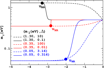
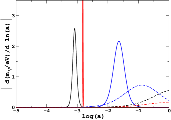
Starting at , the function decreases from 1 to 0, with a velocity that depends on . The top panel in Figure 1 gives the behavior of eq. (18) with different parameters; the bottom panels shows that in this parametrization, the derivative of the mass with respect to e-fold number resembles a Gaussian function. The peak of the quantity occurs at the value ; hence, for , the mass variation takes place immediately after the non-relativistic transition () and lasts a fraction of e-folds (roughly, e-folds); for the variation is smooth and centered on some intermediate redshift between and 0; while for , the transition is still on-going today, and the present epoch roughly coincides with the maximum variation.
 |
 |
Although the functional form of , eq. (III.2), seems complicated, one should note that it is one of the simplest forms satisfying our requirements with a minimal number of parameters. An example that could look simpler, but that for practical purposes is not, would be to assume that the two plateaus are linked together by a straight line. In this case, we would need a parameterization of the form
where corresponds to the chosen redshift in which the transition stops. Notice that in this case not only we still have three parameters to describe the mass variation, but also the function is not smoooth. Moreover, the derivative of the mass with respect to gives a top-hat-like function which is discontinuous at both and . In this sense, it seemed to us that equation (18) would give us the best “price-to-earnings ratio” among the possibilities to use phenomenologically motivated parameterizations for the mass-varying neutrinos, although certainly there could be similar proposals equally viable, such as for instance the possibility of adapting for the mass variation the parameterization used for the dark energy equation of state in Douspis:2006rs ; Linden:2008mf . There, the transition between two constant values of the equation of state exhibits a dependence, where is responsible for the duration of the transition and is related to its half-way point.
In the rest of our analysis, we will use a couple of extra assumptions that need to be taken into account when going through our results. First, we will consider that only one of the three neutrino species is interacting with the dark energy field, that is, only one of the mass eigenstates has a variable mass. The reason for this approximation is twofold: it is a simpler case (compared to the case with 3 varying-mass neutrinos), since instead of 6 extra parameters with respect to the case of constant mass, we have only 2, namely the early mass of the neutrino whose mass is varying, , and the velocity of the transition, related to .
Besides simplicity, the current choice is the only one allowed presently in the case in which neutrinos were heavier in the past. Indeed, we expect our stronger constraints to come from those scenarios, especially if the neutrino species behaves as a nonrelativistic component at the time of radiation-matter equality, given by (here the indexes and stand for cold dark matter and baryons, respectively, and is the effective number of relativistic neutrinos). Taking the three neutrino species to be nonrelativistic at equality would change significantly the value of , contradicting CMB data (according to WMAP5, (68 C.L.) Komatsu:2008hk ). Instead, a single neutrino species is still marginally allowed to be non-relativistic at that time.
To simplify the analysis, we also assumed that the dark energy field, when not interacting with the neutrinos, reached already the so-called scaling solution (see, e.g., DEreview1 and references therein), i.e., the dark energy equation of state in eq. (15) is constant in the absence of interaction. Notice however that when the neutrinos become non-relativistic the dark energy fluid receives the analogous of the chameleon kicks we mentioned before, and the dark energy effective equation of state, eq. (III.1), does vary for this period in a consistent way.
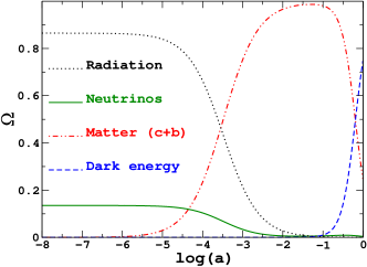
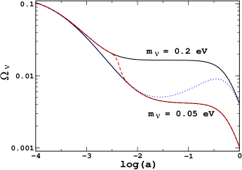
The upper panel of Figure 2 shows how the density parameters of the different components of the universe evolve in time, in a typical MaVaNs model. The lower panel displays a comparison between mass-varying and constant mass models, in particular during the transition from to . As one would expect, far from the time of the transition, the densities evolve as they would do in the constant mass case.
 |
 |
III.3 Perturbation equations
The next step is to calculate the cosmological perturbation equations and their evolution using this parameterization. We chose to work in the synchronous gauge, and our conventions follow the ones by Ma and Bertschinger Ma:1995ey . In this case, the perturbed metric is given by
| (20) |
In this gauge, the equation for the three-momentum of the neutrinos reads Ichiki:2007ng
| (21) |
where, as in equation (4), we define
| (22) |
Since the neutrino phase space distribution Ma:1995ey can be written as , one can show that the first order Boltzmann equation for a massive neutrino species, after Fourier transformation, is given by Brookfield:2005bz ; Ichiki:2007ng
where and are the synchronous potentials in the Fourier space. Notice that the perturbed neutrino energy density and pressure are also going to be modified due to the interaction, and are written as
| (24) | |||||
| (25) |
This extra term comes from the fact that the comoving energy depends on the dark energy density, leading to an extra-term which is proportional to .
Moreover, if we expand the perturbation in a Legendre series Ma:1995ey , the neutrino hierarchy equations will read,
| (26) | |||||
where
| (27) |
For the dark energy, we use the “fluid approach” Hu:1998kj (see also Bean:2003fb ; Hannestad:2005ak ; Koivisto:2005mm ), so that the density and velocity perturbations are given by,
| (28) |
| (29) |
where the dark energy anisotropic stress is assumed to be zero Mota:2007sz , and the sound speed is defined in the frame comoving with the dark energy fluid Weller:2003hw . So, in the synchronous gauge, the quantity is related to through
| (30) |
In addition, from eqs. (15) and (22), we have that
| (31) |
IV Results and Discussion
IV.1 Numerical approach
Equipped with the background and perturbation equations, we can study this scenario by modifying the numerical packages that evaluate the CMB anisotropies and the matter power spectrum. In particular, we modified the CAMB code111http://camb.info/ Lewis:1999bs , based on CMBFast222http://cfa-www.harvard.edu/mzaldarr/CMBFAST/cmbfast.html Seljak:1996is routines. We use CosmoMC333http://cosmologist.info/cosmomc/ Lewis:2002ah in order to sample the parameter space of our model with a Markov Chain Monte Carlo (MCMC) technique.
We assume a flat universe, with a constant equation of state dark energy fluid, cold dark matter, 2 species of massless neutrinos plus a massive one, and ten free parameters. Six of them are the standard CDM parameters, namely, the physical baryon density , the physical cold dark matter density , the dimensionless Hubble constant , the optical depth to reionization , the amplitude () and spectral index () of primordial density fluctuations. In addition, we vary the constant dark energy equation of state parameter and the three parameters accounting for the neutrino mass: the present mass , the logarithm of the parameter related to the duration of the transition, and the logarithm of the ratio of the modulus of the mass difference over the current mass, , where we define
All these parameters take implicit flat priors in the regions in which they are allowed to vary (see Table 1).
| Parameter | Range |
|---|---|
| Region 95 (68) C.L. | Region 95 (68) C.L. | |
| () | () | |
| (eV) | () | () |
| — | ||
| — | ||
Concerning the last parameter, notice that we choose to divide the parameter space between two regions: one in which the mass is decreasing over time () and one in which it is increasing (). We chose to make this separation because the impact on cosmological observables is different in each regime, as we will discuss later, and by analyzing this regions separately we can gain a better insight of the physics driving the constraints in each one of them. Moreover, we do not allow for models with , since we are only considering scalar field models with standard kinetic terms.
For given values of all these parameters, our modified version of CAMB first integrates the background equations backward in time, in order to find the initial value of leading to the correct dark energy density today. This problem does not always admit a solution leading to well-behaved perturbations: the dark energy perturbation equations (28), (29) become singular whenever one of the two quantities, or , appearing in the denominators vanishes. As we shall see later, in the case in which the neutrino mass decreases, the background evolution is compatible with cases in which the dark energy density crosses zero, while the second term can never vanish. We exclude singular models by stopping the execution of CAMB whenever , and giving a negligible probability to these models in CosmoMC. The physical interpretation of these pathological models will be explained in the next sections. For other models, CAMB integrates the full perturbation equations, and passes the CMB and matter power spectra to CosmoMC for comparison with the data.
We constrain this scenario using CMB data (from WMAP 5yr Komatsu:2008hk ; Dunkley:2008ie , VSA Scott:2002th , CBI Pearson:2002tr and ACBAR Kuo:2002ua ); matter power spectrum from large scale structure (LSS) data (2dFGRS Cole:2005sx and SDSS Tegmark:2006az ); supernovae Ia (SN) data from Union2008 , and the HST Key project measurements of the Hubble constant freedman01 444While this work was being finished, the SHOES (Supernova, HO, for the Equation of State) Team Riess:2009pu reduced the uncertainty on the Hubble constant by more than a factor 2 with respect to the value obtained by the HST Key Project, finding km s-1 Mpc-1. However, since we are taking a flat prior on , and our best fit value for is contained in their 1 region, we do not expect our results to be strongly affected by their results..
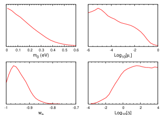
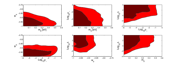
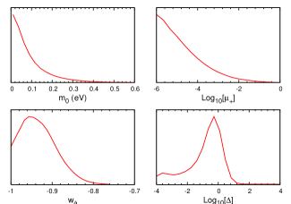
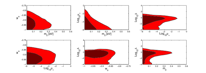
Once the posterior probability of all ten parameters has been obtained, we can marginalize over all but one or two of them, to obtain one- or two-dimensional probability distributions. We verified that the confidence limits on the usual six parameters do not differ significantly from what is obtained in the “vanilla model” Komatsu:2008hk , and therefore we only provide the results for the extra neutrino and dark energy parameters (Figures 7, 6, 4, 3, and Table 2).
IV.2 Increasing neutrino mass
In this model, the background evolution of the dark energy component obeys to equation (15), which reads after division by :
where the two positive quantities and represent respectively the dilution rate and interaction rate of the dark energy density. For any parameter choice, can only decrease with time, so that the integration of the dark energy background equation backward in time always find well-behaved solutions with positive values of . Moreover, the quantity appearing in the denominator of the dark energy perturbation equations is equal to the contribution of the dilution rate to the total energy loss rate, . This quantity is by construction greater than zero, and the dark energy equations cannot become singular. However, when the the interaction rate becomes very large with respect to the dilution rate, this denominator can become arbitrarily close to zero. Then, the dark energy perturbations can be enhanced considerably, distorting the observable spectra and conflicting the data. Actually, this amplification mechanism is well-known and was studied by various authors Bean:2007ny ; Valiviita2008 ; Gavela2009 . It was found to affect the largest wavelengths first, and is usually refered as the large scale instability of coupled dark energy models. The condition for avoiding this instability can be thought to be roughly of the form
| (33) |
where is some number depending on the cosmological parameters and on the data set (since a given data set tells how constrained is the large scale instability, i.e. how small can be the denominator , i.e. how small should the interaction rate remain with respect to the dilution rate). The perturbations are amplified when the denominator is much smaller than one, so should be a number much greater than one. Intuitively, the condition (39) will lead to the rejection of models with small values of (, ) and large values of . Indeed, the interaction rate is too large when the mass variation is significant (large ) and rapid (small ). The dilution rate is too small when is small (close to the cosmological constant limit). Because of that, it seems that when the dark energy equation of state is allowed to vary one can obtain a larger number of viable models if early on in the cosmological evolution Majerotto:2009np ; Valiviita:2009nu .
We ran CosmoMC with our full data set in order to see how much this mass-varying scenario can depart from a standard cosmological model with a fixed dark energy equation of state and massive neutrinos. In our parameter basis, this standard model corresponds to the limit , with whatever value of . The observational signature of a neutrino mass variation during dark energy or matter domination is encoded in well-known effects, such as: (i) a modification of the small-scale matter power spectrum [due to a different free-streaming history], or (ii) a change in the time of matter/radiation equality [due to a different correspondence between the values of (, , ) today and the actual matter density at the time of equality]. On top of that, the neutrino and dark energy perturbations can approach the regime of large-scale instability discussed above.
Our final results - namely, the marginalized 1D and 2D parameter probabilities - are shown in figures 3 and 4. The shape of the contours in space is easily understandable with analytic approximations. The necessary condition (33) for avoiding the large-scale instability reads in terms of our model parameters
| (34) |
where we expressed the mass variation as
| (35) |
Two limits can be clearly seen from this equations. For (fast transitions), the upper limit on reads
| (36) |
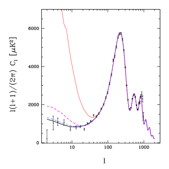
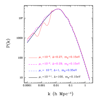
This corresponds to the diagonal limit in the lower half of the right upper panel of figure 4. In fact, the appearance of the large-scale instability is seen in models localized at the edge of the allowed region, as shown in figure 5.
In the opposite case of a very slow transition, , it is clear from eq. (34) that the limit on should be independent on ,
| (37) |
This limit corresponds to the almost vertical cut in the upper part of the plane (upper right panel, fig. 4).
These conditions are easier to satisfy when at the time of the transition, is large. So, in order to avoid the instability, large values of are preferred. However, it is well-known that cosmological observables (luminosity distance relation, CMB and LSS power spectra) better fit the data for close to (cosmological constant limit). In the present model, the role of the large-scale instability is to push the best-fit value from -1 to -0.96, but is still allowed at the 68% C.L.
The main result of this section is that the variation of the neutrino mass is bounded to be small, not so much because of the constraining power of large-scale structure observations in the regime where neutrino free-streaming is important (i.e., small scales), but by CMB and LSS data on the largest scales, which provide limits on the possible instability in DE and neutrino perturbations.
Indeed, for the allowed models, the mass variation could be at most of order 10 for masses around eV, and less than 1 for masses larger than eV: this is undetectable with small scale clustering data, showing that the limit really comes from large scales.
With those results, we conclude that there is no evidence for a neutrino mass variation coming from the present data. In fact, as for most cosmological data analyses, the concordance CDM model remains one of the best fits to the data, lying within the 68 interval of this analysis.
Nonetheless, better constraints will possibly be obtained with forthcoming data, especially the ones that probe patches of the cosmological “desert” between and , like CMB weak lensing Lesgourgues:2005yv , and/or cross-correlations of different pieces of data, like CMB and galaxy-density maps Lesgourgues:2007ix . We can estimate, for instance, what is the favored redshift range for the neutrino mass variation according to our results. Taking eV and the mean likelihood values for and , one can see that the bulk of the mass variation takes place around , a redshift that possibly will be probed by future tomographic probes like weak lensing Hannestad:2006as ; Kitching:2008dp and especially 21 cm absorption lines Loeb:2003ya ; Loeb:2008hg ; Mao:2008ug ; Pritchard:2008wy . Those will help not only to disentangle some degeneracies in the parameter space, but will also allow for direct probes of the neutrino mass in different redshift slices.
IV.3 Decreasing neutrino mass
In this case, the evolution rate of the dark energy density is still given by equation (IV.2) but with an opposite sign for the interaction rate: in can be summarized as
| (38) |
with and both positive. In principle, the interaction rate could overcome the dilution rate, leading to an increase of . Hence, the integration of the dark energy evolution equation backward in time can lead to negative values of , and the prior implemented in our CAMB version is relevant. Still, the denominator can never vanish since it is equal to .
Well before before the transition, the interaction rate is negligible and is always negative. We conclude that starts from small positive values and increases. If the condition
| (39) |
is violated during the transition, will cross zero and become positive. This corresponds to growing from zero to , and from to some finite negative value. After has reached its maximum, undergoes the opposite evolution. Reaching is only possible if has a non-monotonic evolution, i.e. if (39) is violated. However, the perturbations diverge even before reaching this singular point: when tends to infinity, it is clear from eq. (III.3) that the neutrino perturbation derivatives become arbitrarily large. We conclude that in this model, the condition (39) is a necessary condition for avoiding instabilities, but not a sufficient condition: the data is expected to put a limit on the largest possible value of , which will always be reached before changes sign, i.e. before the inequality (39) is saturated. Hence, the condition for avoiding the instability is intuitively of the form of (33), but now with being a number smaller than one.
We then ran CosmoMC with the full data set and obtained the marginalized 1D and 2D parameter probabilities shown in figures 6 and 7. The major differences with respect to the increasing mass case are: a stronger bound on , a much stronger bound on , and the fact that large values of are now excluded. This can be understood as follows. In order to avoid instabilites, it is necessary to satisfy the inequalities (36), (37), but with a much smaller value of than in the increasing mass case; hence, the contours should look qualitatively similar to those obtained previously, but with stronger bounds. This turns out to be the case, although in addition, large values are now excluded. Looking at the mass variation for large in figure 1, we see that in this limit the energy transfer takes place essentially at low redhsift. Hence, the interaction rate is large close to . In many models, this leads to positive values of at the present time, to a non-monotonic behavior of the dark energy density, and to diverging perturbations. This can only be avoided when is large with respect to -1, i.e. when the dilution rate is enhanced. Hence, in this model, the need to avoid diverging perturbations imposes a strong parameter correlation between and . However, values of greater than -0.8 are not compatible with the supernovae, CMB and LSS data set; this slices out all models with large .
The fact that the bound on is stronger in the decreasing mass case is also easily understandable: for the same value of the mass difference , a given corresponds to a larger mass in the decreasing mass case. It is well-known that CMB and LSS data constrain the neutrinos mass through its background effect, i.e. through its impact on the time of matter/radiation equality for a given dark matter abundance today. The impact is greater when is larger, i.e. in the decreasing mass case; therefore, the bounds on are stronger.
V Concluding remarks
In this work we analysed some mass-varying neutrino scenarios in a nearly model independent way, using a general and well-behaved parameterization for the neutrino mass, including variations in the dark energy density in a self-consistent way, and taking neutrino/dark energy perturbations into account.
Our results for the background, CMB anisotropies, and matter power spectra are in agreement with previous analyses of particular scalar field models, showing that the results obtained with this parameterization are robust and encompass the main features of the MaVaNs scenario.
Moreover, a comparison with cosmological data shows that only small mass variations are allowed, and that MaVaNs scenario are mildly disfavored with respect to the constant mass case, especially when neutrinos become lighter as the universe expands. In both cases, neutrinos can change significantly the evolution of the dark energy density, leading to instabilities in the dark energy and/or neutrino perturbations when the transfer of energy between the two components per unit of time is too large. These instabilities can only be avoided when the mass varies by a very small amount, especially in the case of a decreasing neutrino mass. Even in the case of increasing mass, constraining better the model with forthcoming data will be a difficult task, since it mimics a massless neutrino scenario for most of the cosmological time.
One should keep in mind that our analysis assumes a constant equation of state for dark energy and a monotonic behavior for the mass variation. Even though those features are present in most of the simplest possible models, more complicated models surely can evade the constraints we obtained in our analysis.
Finally, those constraints will improve with forthcoming tomographic data. If any of the future probes indicate a mismatch in the values of the neutrino mass at different redshifts, we could arguably have a case made for the mass-varying models.
Acknowledgments
We would like to thank Luca Amendola, Alberto Fernández-Soto, Gennaro Miele, Miguel Quartin, Rogerio Rosenfeld, and José W.F. Valle for discussions concerning an earlier version of this work. This work was supported by the European Union (contracts No. RII3-CT-2004-506222 and MRTN-CT-2004-503369, Marie Curie Training Network “UniversetNet” MRTN-CT-2006-035863), by the Spanish grants FPA2008-00319 (MEC) and PROMETEO/2009/091 (Generalitat Valenciana), and by a MEC-IN2P3 agreement. UF is supported by an I3P-CSIC fellowship. This work made some progress during a fruitful stay at the Galileo Galilei Institute for Theoretical Physics, supported by INFN. We also acknowledge the use of the Legacy Archive for Microwave Background Data Analysis (LAMBDA). Support for LAMBDA is provided by the NASA Office of Space Science.
References
- (1) A. G. Riess et al. [Supernova Search Team Collaboration], Astron. J. 116, 1009 (1998) [arXiv:astro-ph/9805201].
- (2) S. Perlmutter et al. [Supernova Cosmology Project Collaboration], Astrophys. J. 517, 565 (1999) [arXiv:astro-ph/9812133].
- (3) J. Frieman, M. Turner and D. Huterer, Ann. Rev. Astron. Astrophys. 46, 385 (2008) [arXiv:0803.0982 [astro-ph]].
- (4) E. J. Copeland, M. Sami and S. Tsujikawa, Int. J. Mod. Phys. D 15, 1753 (2006) [arXiv:hep-th/0603057].
- (5) P. J. E. Peebles and B. Ratra, Rev. Mod. Phys. 75, 559 (2003) [arXiv:astro-ph/0207347].
- (6) R. R. Caldwell and M. Kamionkowski, Annu. Rev. Nucl. Part. Sci. 59, 397 (2009) [arXiv:0903.0866 [astro-ph.CO]]
- (7) R. R. Caldwell, R. Dave and P. J. Steinhardt, Phys. Rev. 80, 1582 (1998) [arXiv:astro-ph/9708069].
- (8) E. V. Linder, Rept. Prog. Phys. 71, 056901 (2008) [arXiv:0801.2968 [astro-ph]].
- (9) A. Albrecht et al., “Report of the Dark Energy Task Force,” arXiv:astro-ph/0609591.
- (10) P. Gu, X. Wang and X. Zhang, Phys. Rev. D 68, 087301 (2003) [arXiv:hep-ph/0307148].
- (11) R. Fardon, A. E. Nelson and N. Weiner, JCAP 0410, 005 (2004) [arXiv:astro-ph/0309800].
- (12) R. D. Peccei, Phys. Rev. D 71, 023527 (2005) [arXiv:hep-ph/0411137].
- (13) L. Amendola, M. Baldi and C. Wetterich, Phys. Rev. D 78, 023015 (2008) [arXiv:0706.3064 [astro-ph]].
- (14) C. Wetterich, Phys. Lett. B 655, 201 (2007) [arXiv:0706.4427 [hep-ph]].
- (15) S. Hannestad, Ann. Rev. Nucl. Part. Sci. 56, 137 (2006) [arXiv:hep-ph/0602058].
- (16) J. Lesgourgues and S. Pastor, Phys. Rept. 429, 307 (2006) [arXiv:astro-ph/0603494].
- (17) N. Afshordi, M. Zaldarriaga and K. Kohri, Phys. Rev. D 72, 065024 (2005) [arXiv:astro-ph/0506663].
- (18) O. E. Bjaelde, A. W. Brookfield, C. van de Bruck, S. Hannestad, D. F. Mota, L. Schrempp and D. Tocchini-Valentini, JCAP 0801, 026 (2008) [arXiv:0705.2018 [astro-ph]].
- (19) R. Bean, E. E. Flanagan and M. Trodden, New J. Phys. 10, 033006 (2008) [arXiv:0709.1124 [astro-ph]].
- (20) R. Bean, E. E. Flanagan and M. Trodden, Phys. Rev. D 78, 023009 (2008) [arXiv:0709.1128 [astro-ph]].
- (21) R. Bean, E. E. Flanagan, I. Laszlo and M. Trodden, Phys. Rev. D 78, 123514 (2008) [arXiv:0808.1105 [astro-ph]].
- (22) A. E. Bernardini and O. Bertolami, Phys. Lett. B 662, 97 (2008) [arXiv:0802.4449 [hep-ph]].
- (23) A. W. Brookfield, C. van de Bruck, D. F. Mota and D. Tocchini-Valentini, Phys. Rev.Lett. 96, 061301 (2006) [arXiv:astro-ph/0503349].
- (24) A. W. Brookfield, C. van de Bruck, D. F. Mota and D. Tocchini-Valentini, Phys. Rev. D 73, 083515 (2006) [Erratum-ibid. D 76, 049901 (2007)] [arXiv:astro-ph/0512367].
- (25) K. Ichiki and Y. Y. Keum, JCAP 0806, 005 (2008) [arXiv:0705.2134 [astro-ph]].
- (26) G. B. Zhao, J. Q. Xia and X. M. Zhang, JCAP 0707, 010 (2007) [arXiv:astro-ph/0611227].
- (27) G. W. Anderson and S. M. Carroll, arXiv:astro-ph/9711288.
- (28) L. Amendola, Phys. Rev. D 62, 043511 (2000) [arXiv:astro-ph/9908023].
- (29) L. Amendola and D. Tocchini-Valentini, Phys. Rev. D 64, 043509 (2001) [arXiv:astro-ph/0011243].
- (30) G. R. Farrar and P. J. E. Peebles, Astrophys. J. 604, 1 (2004) [arXiv:astro-ph/0307316].
- (31) U. França and R. Rosenfeld, Phys. Rev. D 69, 063517 (2004) [arXiv:astro-ph/0308149].
- (32) G. Huey and B. D. Wandelt, Phys. Rev. D 74, 023519 (2006) [arXiv:astro-ph/0407196].
- (33) S. Das, P. S. Corasaniti and J. Khoury, Phys. Rev. D 73, 083509 (2006) [arXiv:astro-ph/0510628].
- (34) M. Quartin, M. O. Calvao, S. E. Joras, R. R. R. Reis and I. Waga, JCAP 0805, 007 (2008) [arXiv:0802.0546 [astro-ph]].
- (35) G. La Vacca, J. R. Kristiansen, L. P. L. Colombo, R. Mainini and S. A. Bonometto, JCAP 0904, 007 (2009) [arXiv:0902.2711 [astro-ph.CO]].
- (36) M. Chevallier and D. Polarski, Int. J. Mod. Phys. D 10, 213 (2001) [arXiv:gr-qc/0009008].
- (37) E. V. Linder, Phys. Rev. Lett. 90, 091301 (2003) [arXiv:astro-ph/0208512].
- (38) G. Mangano, G. Miele, S. Pastor, T. Pinto, O. Pisanti and P. D. Serpico, Nucl. Phys. B 729, 221 (2005) [arXiv:hep-ph/0506164].
- (39) R. Rosenfeld, Phys. Rev. D 75, 083509 (2007) [arXiv:astro-ph/0701213].
- (40) P. Brax, C. van de Bruck, A. C. Davis, J. Khoury and A. Weltman, Phys. Rev. D 70, 123518 (2004) [arXiv:astro-ph/0408415].
- (41) P. S. Corasaniti and E. J. Copeland, Phys. Rev. D 67, 063521 (2003) [arXiv:astro-ph/0205544].
- (42) M. Douspis, Y. Zolnierowski, A. Blanchard and A. Riazuelo, Astron. and Astrophys. 488, 47 (2008) [arXiv:astro-ph/0602491].
- (43) S. Linden and J. M. Virey, Phys. Rev. D 78, 023526 (2008) [arXiv:0804.0389 [astro-ph]].
- (44) E. Komatsu et al. [WMAP Collaboration], Astrophys. J. Suppl. 180, 330 (2009) [arXiv:0803.0547 [astro-ph]].
- (45) C. P. Ma and E. Bertschinger, Astrophys. J. 455, 7 (1995) [arXiv:astro-ph/9506072].
- (46) W. Hu, Astrophys. J. 506, 485 (1998) [arXiv:astro-ph/9801234].
- (47) R. Bean and O. Dore, Phys. Rev. D 69, 083503 (2004) [arXiv:astro-ph/0307100].
- (48) S. Hannestad, Phys. Rev. D 71, 103519 (2005) [arXiv:astro-ph/0504017].
- (49) T. Koivisto and D. F. Mota, Phys. Rev. D 73, 083502 (2006) [arXiv:astro-ph/0512135].
- (50) D. F. Mota, J. R. Kristiansen, T. Koivisto and N. E. Groeneboom, Mon. Not. R. Astron. Soc. 382, 793 (2007) [arXiv:0708.0830 [astro-ph]].
- (51) J. Weller and A. M. Lewis, Mon. Not. Roy. Astron. Soc. 346, 987 (2003) [arXiv:astro-ph/0307104].
- (52) A. Lewis, A. Challinor and A. Lasenby, Astrophys. J. 538, 473 (2000) [arXiv:astro-ph/9911177].
- (53) U. Seljak and M. Zaldarriaga, Astrophys. J. 469, 437 (1996) [arXiv:astro-ph/9603033].
- (54) A. Lewis and S. Bridle, Phys. Rev. D 66, 103511 (2002) [arXiv:astro-ph/0205436].
- (55) J. Dunkley et al. [WMAP Collaboration], Astrophys. J. Suppl. 180, 306 (2009) [arXiv:0803.0586 [astro-ph]].
- (56) P. F. Scott et al., Mon. Not. Roy. Astron. Soc. 341, 1076 (2003) [arXiv:astro-ph/0205380].
- (57) T. J. Pearson et al., Astrophys. J. 591, 556 (2003) [arXiv:astro-ph/0205388].
- (58) C. l. Kuo et al. [ACBAR collaboration], Astrophys. J. 600, 32 (2004) [arXiv:astro-ph/0212289].
- (59) S. Cole et al. [The 2dFGRS Collaboration], Mon. Not. Roy. Astron. Soc. 362, 505 (2005) [arXiv:astro-ph/0501174].
- (60) M. Tegmark et al. [SDSS Collaboration], Phys. Rev. D 74, 123507 (2006) [arXiv:astro-ph/0608632].
- (61) M. Kowalski et al. [Supernova Cosmology Project Collaboration], Astrophys. J. 686, 749 (2008) [arXiv:0804.4142 [astro-ph]].
- (62) W. L. Freedman et al., Astrophys. J. 553, 47 (2001) [arXiv:astro-ph/0012376].
- (63) A. G. Riess et al., Astrophys. J. 699, 539 (2009) [arXiv:0905.0695 [astro-ph.CO]].
- (64) J. Valiviita, E. Majerotto and R. Maartens, JCAP 0807, 020 (2008) [arXiv:0804.0232 [astro-ph]].
- (65) M. B. Gavela, D. Hernandez, L. L. Honorez, O. Mena and S. Rigolin, JCAP 0907, 034 (2009) [arXiv:0901.1611 [astro-ph]].
- (66) J. Valiviita, R. Maartens and E. Majerotto, arXiv:0907.4987 [astro-ph.CO].
- (67) E. Majerotto, J. Valiviita and R. Maartens, arXiv:0907.4981 [astro-ph.CO].
- (68) J. Lesgourgues, L. Perotto, S. Pastor and M. Piat, Phys. Rev. D 73, 045021 (2006) [arXiv:astro-ph/0511735].
- (69) J. Lesgourgues, W. Valkenburg and E. Gaztañaga, Phys. Rev. D 77, 063505 (2008) [arXiv:0710.5525 [astro-ph]].
- (70) S. Hannestad, H. Tu and Y. Y. Y. Wong, JCAP 0606, 025 (2006) [arXiv:astro-ph/0603019].
- (71) T. D. Kitching, A. F. Heavens, L. Verde, P. Serra and A. Melchiorri, Phys. Rev. D 77, 103008 (2008) [arXiv:0801.4565 [astro-ph]].
- (72) A. Loeb and M. Zaldarriaga, Phys. Rev. Lett. 92, 211301 (2004) [arXiv:astro-ph/0312134].
- (73) A. Loeb and J. S. Wyithe, Phys. Rev. Lett. 100, 161301 (2008) [arXiv:0801.1677 [astro-ph]].
- (74) Y. Mao, M. Tegmark, M. McQuinn, M. Zaldarriaga and O. Zahn, Phys. Rev. D 78, 023529 (2008) [arXiv:0802.1710 [astro-ph]].
- (75) J. R. Pritchard and E. Pierpaoli, Phys. Rev. D 78, 065009 (2008) [arXiv:0805.1920 [astro-ph]].