Sensitivity of galaxy cluster dark energy constraints to halo modeling uncertainties

Abstract

We perform a sensitivity study of dark energy constraints from galaxy cluster surveys to uncertainties in the halo mass function, bias and the mass–observable relation. For a set of idealized surveys, we evaluate cosmological constraints as priors on sixteen nuisance parameters in the halo modeling are varied. We find that surveys with a higher mass limit are more sensitive to mass–observable uncertainties while surveys with low mass limits that probe more of the mass function shape and evolution are more sensitive to mass function errors. We examine the correlations among nuisance and cosmological parameters. Mass function parameters are strongly positively (negatively) correlated with $\Omega_{\rm DE}$ ($w$). For the mass–observable parameters, $\Omega_{\rm DE}$ is most sensitive to the normalization and its redshift evolution while $w$ is more sensitive to redshift evolution in the variance. While survey performance is limited mainly by mass–observable uncertainties, the current level of mass function error is responsible for up to a factor of two degradation in ideal cosmological constraints. For surveys that probe to low masses ($10^{13.5}h^{-1}M_{\odot}$), even percent-level constraints on model nuisance parameters result in a degradation of $\sim\sqrt{2}$ (2) on $\Omega_{\rm DE}$ ($w$) relative to perfect knowledge.

I Introduction

The spatial abundance of galaxy clusters is a potentially powerful approach to test the nature of dark energy (Cunha et al., 2009; Sahlén et al., 2009; Voit, 2005; Battye and Weller, 2003; Rosati et al., 2002; Haiman et al., 2001; Marian and Bernstein, 2006). As is the case for all dark energy probes, modeling and other systematic uncertainties in the data analysis must be identified and controlled. The primary uncertainties for cluster counts involve theoretical modeling of the halo space density as a function of mass — the mass function — along with uncertainties associated with modeling the halo mass selection function of a specific survey.

While recent studies have derived consistent and competitive cosmological constraints using X-ray Mantz et al. (2008); Vikhlinin et al. (2009); Henry et al. (2009) and optical Gladders et al. (2007); Rozo et al. (2009) cluster surveys, the larger volume and improved sensitivity of upcoming surveys motivate a stronger effort to study sources of systematic error. Early work on forecasting cluster constraints focused attention on systematics arising from the mass–observable relation (Levine et al. (2002); Majumdar and Mohr (2003, 2004), etc.). These errors fall into two categories: i) bias arising from uncertain knowledge of the normalization and ii) mass variance at fixed observable signal or, equivalently, scatter in the mass-signal relation. The redshift evolution of these effects are particularly important Lima and Hu (2004, 2005, 2007); Cunha (2009). If the scatter is large, the functional form of the mass–observable likelihood becomes important (Shaw et al., 2009).

Uncertainties in the mass–observable relation can be characterized with a combination of empirical and theoretical approaches. For example, the slope and normalization of the intracluster gas thermal energy can be probed with X-ray and Sunyaev-Zel’dovich (SZ) observations (Arnaud et al., 2005; Maughan et al., 2006; Vikhlinin et al., 2006; Morandi et al., 2007; Bonamente et al., 2008; Zhang et al., 2008; Pratt et al., 2009) while the variance and evolution with redshift can be predicted in a model-dependent manner using multi-fluid simulations (Bialek et al., 2001; Borgani et al., 2004; da Silva et al., 2004; Kravtsov et al., 2006; Ascasibar et al., 2006; Muanwong et al., 2006; Puchwein et al., 2008; Aghanim et al., 2009; Stanek et al., 2009). For example, a ‘preheated’ gas treatment that matches the low-redshift X-ray luminosity–temperature relation predicts weakly increasing scatter in the integrated thermal SZ signal at fixed mass, from $13\%$ at $z=0$ to $18\%$ at $z=1$ (Stanek et al., 2009).

Theoretical uncertainty in the mass function has not been extensively studied in previous Fisher forecasts. This is partly because mass–observable uncertainties are typically dominant in comparison, and partly because mass function calibrations by the simulation community have been evolving.

The original mass function of Press & Schechter Press and Schechter (1974), derived with support of 1000-particle N-body simulations, has evolved into a number of forms with billion-particle simulation support, among them the Sheth-Tormen Sheth and Tormen (1999), Jenkins Jenkins et al. (2001), Evrard Evrard et al. (2002), Warren Warren et al. (2006) and Tinker Tinker et al. (2008) mass functions. The Warren parameterization has received a recent update based on an ensemble of large-volume simulations. Correction for systematics associated with initial condition generation and other effects lead to an upward revision in the mass function of $\gtrsim 10$ percent at mass scales probed by SZ surveys (Crocce et al., 2009).

Different measures of mass, based on either particle percolation or spherical filtering, are employed by the aforementioned studies (see Cole and Lacey (1996); White (2002); Lukić et al. (2009) for discussion of these mass measures), but all use the filtered linear power spectrum, $\sigma(M)$, as a similarity variable for expressing halo counts and clustering. While the Tinker calibration Tinker et al. (2008) improved the statistical accuracy of the mass function to the 5% level in number density, the effects of gas dynamics, absent in that work, may produce deviations that are larger than this Stanek et al. (2009). We consider $\sim 10\%$ in space density as a reasonable estimate of the current level of uncertainty in the mass function at cluster scales.

The cited mass function calibrations assume a standard $\Lambda$CDM cosmology, with a Gaussian initial density field evolved under general relativity with a cosmological constant. Extensions to non-standard assumptions are emerging (see e.g. Lo Verde et al. (2008); Dalal et al. (2008); Grossi et al. (2009)), but we do not consider them here.

In this paper, we extend previous Fisher studies of dark energy constraints by including theoretical uncertainties in the halo mass function and clustering bias and by employing a more generous treatment of bias and scatter evolution in the mass–observable relation. We frame the analysis in terms of two idealized surveys roughly patterned after the South Pole Telescope (SPT) SZ survey and the Dark Energy Survey (DES) optical survey. Our baseline idealizations, which assume perfect halo selection (100% completeness) above a redshift-independent mass threshold and constant mass–observable scatter, provide a simple, rational basis upon which complexities, in the form of nuisance parameters discussed below, can be added. The “SZ-motivated” survey has a high mass threshold and small mass–observable scatter while the “optical-motivated” case has a lower mass threshold and larger mass scatter. We refer to these simply as ‘SZ’ and ‘optical’ for the remainder of the paper.

Our main aim is to study performance degradation in $\Omega_{\rm DE}$ and $w$ constraints as a function of prior parameter knowledge. We also provide a first look at parameter correlations for the full model, finding them (unsurprisingly) complex. While writing up this work, we learned of a similar study by Wu, Zentner & Wechsler Wu et al. (2009), who address the effect of mass function systematics on the dark energy figure of merit from cluster surveys. Their approach is complementary to ours, in that they adopt a set of independent nuisance parameters to model systematic error in binned representations of the mass function and halo bias. While this non-parametric approach allows them to more easily identify regions of mass and redshift space that most sensitively affect dark energy constraints, a disadvantage is that it disregards correlations between different mass/redshift bins. Wu et al. also explore a time-dependent equation of state, $w(a)$, and express their results in terms of a figure of merit degradation. They do not emphasize the interplay between mass–observable and mass function systematic errors, as we do here.

The paper is organized as follows. In Sec. II we briefly review the formalism for extracting dark energy constraints from cluster counts and variance in counts and present our parameterization of the mass–observable relations, the mass function and galaxy bias. We present results in Sec. III, offer a critique in Sec. IV and conclude in Sec. V.

II DE from cluster counts and clustering

The subject of deriving cosmological constraints from cluster number counts and clustering of clusters has been treated extensively in the literature (see e.g. Cunha (2009); Lima and Hu (2004, 2005, 2007)). In this section we follow closely the approach described in Cunha (2009).

The comoving number density of clusters at a given redshift $z$ with observable in the range $M_{\rm obs}^{\alpha}\leq M_{\rm obs}\leq M_{\rm obs}^{\alpha+1}$ is given by

$$\bar{n}_{\alpha}(z) \equiv \int_{M_{\rm obs}^{\alpha}}^{M_{\rm obs}^{\alpha+1}}\frac{dM_{\rm obs}}{M_{\rm obs}}\int{\frac{dM}{M}}{\frac{d\bar{n}}{d\ln M}}p(M_{\rm obs}|M)$$ (1)

Uncertainties in the redshifts distort the volume element. Assuming photometric techniques are used to determine the redshifts of the clusters (hereafter photo-z’s) and a perfect angular selection the mean number of clusters in a photo-z bin $z^{\rm p}_{i}\leq z^{\rm p}\leq z^{\rm p}_{i+1}$ is

$$\bar{m}_{\alpha,i} = \int_{z^{\rm p}_{i}}^{z^{\rm p}_{i+1}}dz^{\rm p}\int dz\frac{dV}{dz}\bar{n}_{\alpha}W_{i}^{\rm th}(\Omega)p(z^{\rm p}|z)$$ (2)

where $W^{\rm th}_{i}(\Omega)$ is an angular top hat window function. We parameterize the probability of measuring a photometric redshift, $z^{\rm p}$, given the true cluster redshift $z$ as Lima and Hu (2007)

$$p(z^{\rm p}|z) = \frac{1}{\sqrt{2\pi}\sigma_{z}}\exp\left[-y^{2}(z^{\rm p})\right]$$ (3)

where

$$y(z^{\rm p}) \equiv \frac{z^{\rm p}-z-z^{\rm bias}}{\sqrt{2}\sigma_{z}},$$ (4)

$z^{\rm bias}$ is the photometric redshift bias and $\sigma_{z}$ is the scatter in the photo-z’s. We fix the photo-z bias and scatter at $0$ and $0.02$ throughout this paper.

The sample covariance of counts $m_{\alpha,i}$ is, given by (Hu and Kravtsov, 2003)

$$S_{ij} = \langle(m_{\alpha,i}-\bar{m}_{\alpha,i})(m_{\alpha,j}-\bar{m}_{\alpha,j})\rangle$$ (6)

$$= b_{\alpha,i}\bar{m}_{\alpha,i}b_{\alpha,j}\bar{m}_{\alpha,j}$$

$$\times\int{\frac{d^{3}k}{(2\pi)^{3}}}W_{i}^{*}({\bf k})W_{j}({\bf k})\sqrt{P_{i}(k)P_{j}(k)},$$

where $b_{\alpha,i}(z)$ is the average cluster linear bias defined as

$$b_{\alpha,i}(z) = \frac{1}{\bar{n}_{\alpha,i}(z)}\int_{M_{\rm obs}^{\alpha}}^{M_{\rm obs}^{\alpha+1}}\frac{d{M_{\rm obs}}}{M_{\rm obs}}\int\frac{dM}{M}$$ (7)

$$\times\frac{d\bar{n}_{\alpha,i}(z)}{d\ln M}b(M;z)p(M_{\rm obs}|M).$$

$W_{i}^{*}({\bf k})$ is the Fourier transform of the top-hat window function and $P_{i}(k)$ is the linear power spectrum at the centroid of redshift bin $i$. We present our choice for $b(M;z)$ in II.2, when we discuss the parameterization of the errors in the mass function and galaxy bias. We only calculate covariance terms for which $i=j$ since off-diagonal terms are negligible.

Following Lima and Hu (2007), we find that the window function $W_{i}^{*}({\bf k})$ in the presence of photo-z errors is given by

$$W_{i}({\bf k})= 2\exp{\left[ik_{\parallel}\left(r_{i}+\frac{{z^{\rm bias}_{i}}}{{H_{i}}}\right)\right]}\exp{\left[-\frac{{\sigma_{z,i}^{2}k_{\parallel}^{2}}}{{2H_{i}^{2}}}\right]}$$ (8)

$$\times\frac{\sin(k_{\parallel}\delta r_{i}/2)}{k_{\parallel}\delta r_{i}/2}\frac{J_{1}(k_{\perp}r_{i}\theta_{s})}{k_{\perp}r_{i}\theta_{s}}.$$

Here $r_{i}=r(z^{\rm p}_{i})$ is the angular diameter distance to the $i^{\rm th}$ photo-z bin, and $\delta r_{i}=r(z^{\rm p}_{i+1})-r(z^{\rm p}_{i})$. Similarly, $H_{i}=H(z^{\rm p}_{i})=H(z)$, $z^{\rm bias}_{i}=z^{\rm bias}(z^{\rm p}_{i})=z^{\rm bias}(z)$, and $\sigma_{z,i}=\sigma_{z}(z^{\rm p}_{i})=\sigma_{z}(z)$. We assumed that $H(z)$, $z^{\rm bias}(z)$, and $\sigma_{z}(z)$ are constant inside each bin. The variables $k_{\parallel}$ and $k_{\perp}$ represent parallel and perpendicular components of the wavenumber ${\bf k}$ relative to the line of sight.

Define the covariance matrix of halo counts

$$C_{ij}=S_{ij}+{\bar{m}_{i}}\delta_{ij}$$ (9)

where ${\bar{m}_{i}}$ is the vector of mean counts defined in Eq. (2) and $S_{ij}$ is the sample covariance defined in Eq. (6). The indices $i$ and $j$ here run over all mass and redshift bins. Assuming Poisson noise and sample variance are the only sources of noise, the Fisher matrix is, (Hu and Cohn, 2006; Lima and Hu, 2004; Holder et al., 2001)

$$F_{\alpha\beta}=\bar{\bf m}^{t}_{,\alpha}{\bf C}^{-1}\bar{{\bf m}}_{,\beta}+\frac{1}{2}{\rm Tr}[{\bf C}^{-1}{\bf S}_{,\alpha}{{\bf C}}^{-1}{\bf S}_{,\beta}],$$ (10)

where the “,” denote derivatives with respect to the model parameters. The first term on the right-hand side contains the “information” from the mean counts, $\bar{m}$. The $S_{ij}$ matrix only contributes noise to this term, and hence only reduces its information content. The second term contains the information from the sample covariance.

II.1 Systematics in the mass–observable relation

We introduce six degrees of freedom in the sector of the model that links halo mass to an observable signal. We assume a log-normal form for the probability of measuring an observable signal, denoted $M_{\rm obs}$, given true mass $M$,

$$p(M_{\rm obs}|M)=\frac{1}{\sqrt{2\pi}\sigma_{\ln M}}\exp\left[-x^{2}(M_{\rm obs})\right],$$ (11)

where

$$x(M_{\rm obs})\equiv\frac{\ln M_{\rm obs}-\ln M-\ln M_{\rm bias}(M_{\rm obs},z)}{\sqrt{2}\sigma_{\ln M}(M_{\rm obs},z)}.$$ (12)

We model systematic error in the mass proxy by introducing a redshift-dependent bias and variance

$${\rm ln}M_{\rm bias}(z) = B_{0}+B_{1}(1+z),$$ (13)

$$\sigma_{\ln M}^{2}(z) = \sigma_{0}^{2}+\sum_{i=1}^{3}S_{i}z^{i},$$ (14)

where $B_{0}$, $B_{1}$, $\sigma_{0}$ and the three variance coefficients are assumed to be independent of mass. Our default assumption is that $\sigma_{0}$ is non-zero, with values discussed in Sec. II.4, while the remaining parameters have a fiducial value of zero. All six parameters are taken as degrees of freedom and varied in the Fisher analysis presented in Sec. III.

II.2 Systematics in the halo mass function and bias

In the sector of the model describing the halo mass function, we add ten more degrees of freedom. We write the space density of halos as

$$\frac{dn}{dM}=f(\sigma)\frac{\bar{\rho}_{m}}{M}\frac{d\ln\sigma^{-1}}{dM}$$ (15)

and adopt the Tinker parameterization of $f(\sigma)$ (Tinker et al., 2008)

$$f(\sigma)=A\left[\left(\frac{\sigma}{b}\right)^{-a}+1\right]e^{-c/{\sigma^{2}}}.$$ (16)

Following Tinker et al. (2008), we allow the first three parameters of $f(\sigma)$ to vary with redshift, so that

$$A(z)=A_{0}(1+z)^{A_{x}}$$ (17)

$$a(z)=a_{0}(1+z)^{a_{x}}$$ (18)

$$b(z)=b_{0}(1+z)^{-\alpha}$$ (19)

For fiducial parameters, we adopt the values of Tinker et al. (2008) at $\Delta=200$: $A_{0}=0.186$, $A_{x}=-0.14$, $a_{0}=1.47$, $a_{x}=-0.06$, $b_{0}=2.57$, $\log_{10}(\alpha)={(\frac{0.75}{log(\Delta/75)})^{1.2}}$, and $c=1.19$. As Tinker et al. Tinker et al. (2008) explain, A controls the overall amplitude of $f(\sigma)$, $a$ controls the tilt, and $b$ sets the mass scale where the power law in $f(\sigma)$ becomes significant.

We adopt the $b(M,z)$ fit of Sheth and Tormen (1999) for the galaxy bias

$$b(M,z)=1+\frac{a_{c}\delta_{c}^{2}/\sigma^{2}-1}{\delta_{c}}+\frac{2p_{c}}{\delta_{c}[1+(a\delta_{c}^{2}/\sigma^{2})^{p_{c}}]},$$ (20)

and choose the fiducial values for the parameters to be $a_{c}=0.75$, $\delta_{c}=1.69$, and $p_{c}=0.3$.

In total, the mass function and bias introduce ten additional parameters, and we consider all of these as degrees of freedom in the Fisher analysis presented in § III. The assumption that the bias is independent of the mass function is very conservative. Manera et al. Manera et al. (2009) show that, in the range of scales we are interested in, the bias can be predicted to roughly $\sim 10\%$ accuracy given the mass function.

II.3 Fiducial Parameter Values

The fiducial values of the sixteen nuisance parameters are summarized in Table LABEL:tbl:params. These parameters control the underlying counts and clustering of equations (1) and (7) via the explicit forms of equations (11), (15) and (20), and thereby produce the sample covariance, equation (9), and Fisher matrix, equation (10).

Table 1: Halo modeling nuisance parameters

Class	Name	Fid. Value	Notes
	$B_{0}$	0.0	constant bias
	$B_{1}$	0.0	z-dependent bias
$M_{\rm obs}$	$\sigma_{0}^{2}$	0.04,0.625	constant variance
	$S_{1}$	0.0	$z^{1}$ variance
	$S_{2}$	0.0	$z^{2}$ variance
	$S_{3}$	0.0	$z^{3}$ variance
	$A_{0}$	0.186	z-independent
	$a_{0}$	0.147	”
Mass	$b_{0}$	2.57	”
Function	$c$	1.19	”
	$A_{x}$	-0.14	$A(z)=A_{0}(1+z)^{A_{x}}$
	$a_{x}$	-0.06	$a(z)=a_{0}(1+z)^{a_{x}}$
	$\alpha$	0.0107	$b(z)=b_{0}(1+z)^{\alpha}$
	$a_{c}$	0.75	z-independent
Bias	$\delta_{c}$	1.69	”
	$p_{c}$	0.30	”

II.4 Reference Model Surveys

We apply our tests to four distinct surveys consisting of a fiducial and three options. All are assumed to cover a sky area of 4000 square degrees and extend to a limiting redshift $z_{\rm max}=2.0$. The test surveys differ only in two parameters: the mass threshold, $M_{\rm th}$, and the zero–redshift variance in the mass–observable relation, $\sigma_{0}^{2}$.

Our chosen survey parameters, given in Table LABEL:tbl:constraints, represent capabilities likely to be realized in the near future using sub-mm and optical/NIR observations. For example, the South Pole Telescope (SPT) is expected to detect clusters above $M_{\rm th}=10^{14.2}h^{-1}M_{\odot}$ up to a redshift of 2 (see e.g. Carlstrom et al. (2002)), with photometric redshifts available from DES+VISTA imaging, the Blanco Cosmology Survey, and the Magellan Telescope. DES+VISTA will have internal capability to detect clusters optically with techniques known to work above $M_{\rm th}=10^{13.5}h^{-1}M_{\odot}$ (see e.g. Koester et al. (2007) and Johnston et al. (2007)).

We subdivide the sky into 400 bins of 10 sq. degrees each, and calculate the counts and sample variance using mass bins of width $\log(\Delta M_{\rm obs})=0.2$ with the exception of the highest mass bin, which we extend to infinity. We set the width of our redshift bins to $\Delta z^{\rm p}=0.1$. These bin sizes imply 20 redshift bins and 5 bins of mass for the surveys 1 and 2. For Surveys 3 and 4, we divide the mass range $10^{13.5}\leq M_{obs}^{\rm opt}\leq 10^{14.2}h^{-1}M_{\odot}$ into 5 bins and use the same mass binning as the Surveys 1 and 2 for $M_{obs}^{\rm opt}>10^{14.2}h^{-1}M_{\odot}$, with a total of 10 mass bins and 20 redshift bins.

We assume fiducial cosmological parameters based on the fifth year data release of the Wilkinson Microwave Anisotropy Probe (WMAP5, Komatsu et al. (2008)). Thus, we set the baryon density, $\Omega_{b}h^{2}=0.0227$, the dark matter density, $\Omega_{m}h^{2}=0.1326$, the normalization of the power spectrum at $k=0.05{\rm Mpc}^{-1}$, $A_{s}=4.625\times 10^{-5}$, the tilt, $n=0.963$, the optical depth to reionization, $\tau=0.087$, the dark energy density, $\Omega_{\rm DE}=0.742$, and the dark energy equation of state, $w=-1$. In this cosmology, $\sigma_{8}=0.796$.

With the exception of $w$, the cosmological parameters we used have been determined to an accuracy of a few percent. Extrapolating into the future, we assume $1\%$ priors on all cosmological parameters except $\Omega_{\rm DE}$ and $w$. We used CMBfast (Seljak and Zaldarriaga, 1996), version 4.5.1, to calculate the transfer functions. We do not explore time evolution of $w$ in this work. In cosmologies with a time varying equation of state, $w(a)$, the relationship between halo model parameters and the error in principal components of $w(a)$ would differ from that reported here, with redshift terms having a larger impact. An important aim of next generation surveys is to test $w\neq-1$, the degree to which dark energy differs from vacuum energy.

III Results

Table 2: Surveys parameters and constraints on cosmological parameters

				Sharp priors		No priors
Survey	$M_{\rm th}[h^{-1}M_{\odot}]$	$\sigma_{0}$	$N_{\rm tot}$	$\sigma(\Omega_{\rm DE})$	$\sigma(w)$	$\sigma(\Omega_{\rm DE})$	$\sigma(w)$
Fid.	$10^{14.2}$	0.2	8,400	0.010	0.050	0.91	2.19
1	$10^{14.2}$	0.5	16,400	0.0083	0.039	0.82	1.81
2	$10^{13.5}$	0.2	359,600	0.0025	0.011	0.098	0.23
3	$10^{13.5}$	0.5	482,400	0.0023	0.0097	0.22	0.35

The baseline, absolute accuracy in $\Omega_{\rm DE}$ and $w$ measurements from the four test surveys are given in Table LABEL:tbl:constraints. The sharp priors columns represent the ideal condition of perfect knowledge of the mass function and mass–observable relation, i.e., delta function priors on all the mass function and mass–observable relation parameters. The no priors columns give results assuming a high degree of ignorance in parameter values.

From Table LABEL:tbl:constraints, we see that a factor $10^{0.7}$ decrease in the mass threshold, $M_{\rm th}$, improves the constraints on both $\Omega_{\rm DE}$ and $w$ by a factor of $\sim 4$. The improvement results from the increase in cluster counts as well as an increase in the exposed range of the mass function. Surveys 2 and 3 find a factor of 27 and 18 more clusters than the fiducial survey and survey 1, respectively. Increased scatter in $M_{\rm obs}$ results in an increase in counts because of the steepness of the mass function near the $M_{\rm th}$. The negative mass function slope implies that more objects will be up-scattered from below $M_{\rm th}$ than down-scattered. If the scatter is perfectly known, the increase in counts yields better cosmological constraints (Cunha, 2009; Lima and Hu, 2005). This optimistic result must be interpreted with caution. A large mass–observable scatter may reflect poor selection, or contamination by projection or intrinsic sources. Projection is known to produce non-Gaussian features in the mass–observable relation (Cohn, 2006) that can bias constraints if not correctly accounted for (Erickson et al., in prep. Erickson et al. (2009)).

The last columns of Table LABEL:tbl:constraints demonstrate that large degradations in cosmological accuracy result from essentially complete ignorance of the halo modeling parameters. We turn now to study the transition between the regimes of complete knowledge and complete ignorance by varying the prior uncertainties on the sixteen nuisance parameters.

III.1 Degradation from Model Systematic Error

For the parameters controlling the mass–observable relation ($M_{\rm obs}$) and the mass-function/bias (MF/B), we introduce prior uncertainties, $\sigma_{\rm prior}$, that represent errors from previous observation or simulation. Because the $M_{\rm obs}$ and MF/B parameters have different dimensions, we define the priors on them differently, so as to make the prior uncertainties more directly comparable.

We define the prior uncertainty on $M_{\rm obs}$ nuisance parameters, $\sigma_{\rm prior}^{M_{\rm obs}}$, such that the prior $F^{ii}_{\rm prior}$ added to the $i^{\rm th}$ diagonal element of the Fisher matrix is

$$F^{ii}_{\rm prior}=\left(\frac{1}{\sigma_{\rm prior}^{M_{\rm obs}}}\right)^{2}.$$ (21)

The prior uncertainty on an MF/B nuisance parameter, $x_{i}$, is defined as

$$F^{ii}_{\rm prior}=\left(\frac{1}{x_{i}^{2}\sigma_{\rm prior}^{\rm MF/B}}\right)^{2}.$$ (22)

With this definition, $\sigma_{\rm prior}^{\rm MF/B}$ corresponds to the prior fractional uncertainty on each mass-function/bias nuisance parameter. The uncertainties in the $M_{\rm obs}$ nuisance parameters are already fractional since the mass–observable relation is defined in terms of the logarithm of the mass.

Figure 1: The sensitivity of the mass function to variation in Tinker mass function (left panel) and mass–observable (right) parameters is illustrated for redshift $z=0.75$, roughly the median redshift of the surveys considered here. The change in the natural logarithm of number counts as a function of mass is shown while each of the labeled parameters is changed by a fractional amount, $\sigma_{\rm prior}^{\rm MF/B}=0.1$ (left panel) or a fixed amount, $\sigma_{\rm prior}^{M_{\rm obs}}=\pm 0.1$ (right panel). In the latter case, the bias terms are varied by $0.1$ and the variance terms by $-0.1$.

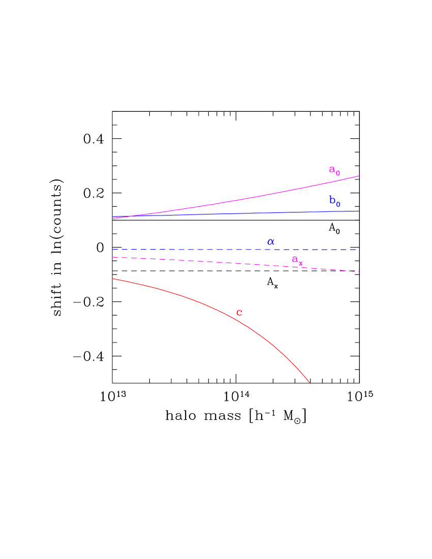
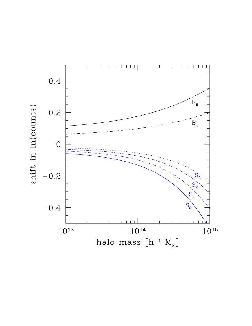
The left plot of Fig. 1 gives a sense of the magnitude of the shifts in number counts as each of the Tinker MF parameters are increased by a fractional amount, $\sigma_{\rm prior}^{\rm MF/B}=0.1$. We evaluate the mass function shifts for the fiducial cosmology at redshift $z=0.75$, roughly the median redshift of our model surveys. Solid lines show the effects of varying the constant terms while dashed lines vary the redshift-dependent factors. At $10^{14}h^{-1}M_{\odot}$, the shift in number ranges from $+0.2$ (varying $a_{0}$) to $-0.3$ (varying $c$). The derivatives are positive for the constant terms, with the exception of $c$, while the derivatives with respect to the $z$-dependent terms are negative. From the figure, we see that a $10\%$ change in $\alpha$ causes very little change in the mass function. However, as we shall see in Sec. III.2, $\alpha$ and the other redshift evolution parameters ($a_{x}$ and $A_{x}$) are nearly perfectly correlated (anti-correlated) with $\Omega_{\rm DE}$ (w), suggesting that the redshift evolution of the mass function needs to be well understood to avoid degradations in cosmological parameter constraints. In the right plot, we show the dependence of the observed mass function on the $M_{\rm obs}$ nuisance parameters, at the same redshift as above. The impact of the $M_{\rm obs}$ nuisance parameters increase with mass because the slope of the mass function increases with mass. The steeper the slope, the more significant is the imbalance between clusters up-scattered or down-scattered into a given mass bin due to bias or scatter in $M_{\rm obs}$.

Figs. 2 and 3 show contours of the multiplicative increase in the errors $\sigma(\Omega_{\rm DE})$ and $\sigma(w)$, respectively, relative to the baseline “Sharp prior” constraints given in Table LABEL:tbl:constraints. The top left panel shows the fiducial survey, with survey 1 (upper right), 2 (lower left) and 3 (lower right) also shown. In all panels, contours show degradation of the error in $\Omega_{\rm DE}$ or $w$ by factors of $2^{j/2}$, with $j$ running from 1 to 8.

Figure 2: Plots of fractional degradation in $\sigma(\Omega_{\rm DE})$ for the Fiducial Survey (top left), Survey 1 (top right), Survey 2 (bottom left), and Survey 3 (bottom right). The contours correspond to regions where constraints on $\Omega_{DE}$ are degraded by factors of $\sqrt{2}$, $2$, $2\sqrt{2}$, $4$, $4\sqrt{2}$, $8$, $8\sqrt{2}$, $16$, relative to the case of perfectly known nuisance parameters. See Table LABEL:tbl:constraints for the baseline constraints on $\Omega_{\rm DE}$.

Figure 3: Plots of fractional degradation in $\sigma(w)$ for the Fiducial Survey (top left), Survey 1 (top right), Survey 2 (bottom left), and Survey 3 (bottom right). The contours correspond to regions where constraints on $w$ are degraded by factors of $\sqrt{2}$, $2$, $2\sqrt{2}$, $4$, $4\sqrt{2}$, $8$, $8\sqrt{2}$, $16$, relative to the case of perfectly known nuisance parameters. See Table LABEL:tbl:constraints for the baseline constraints on $w$.

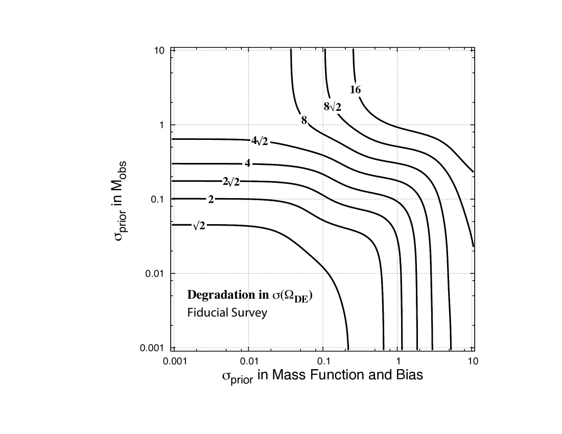
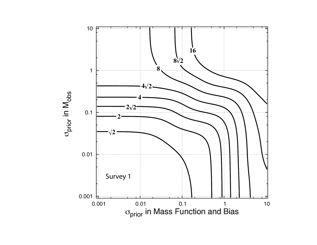
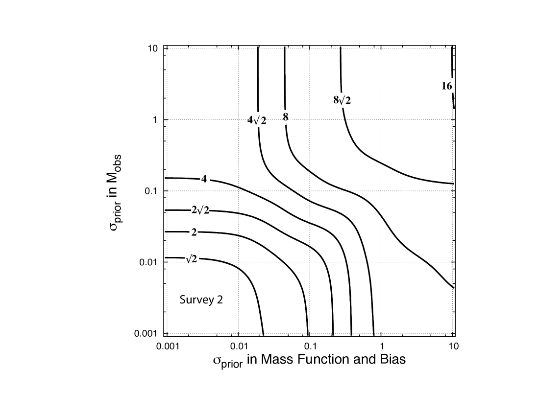
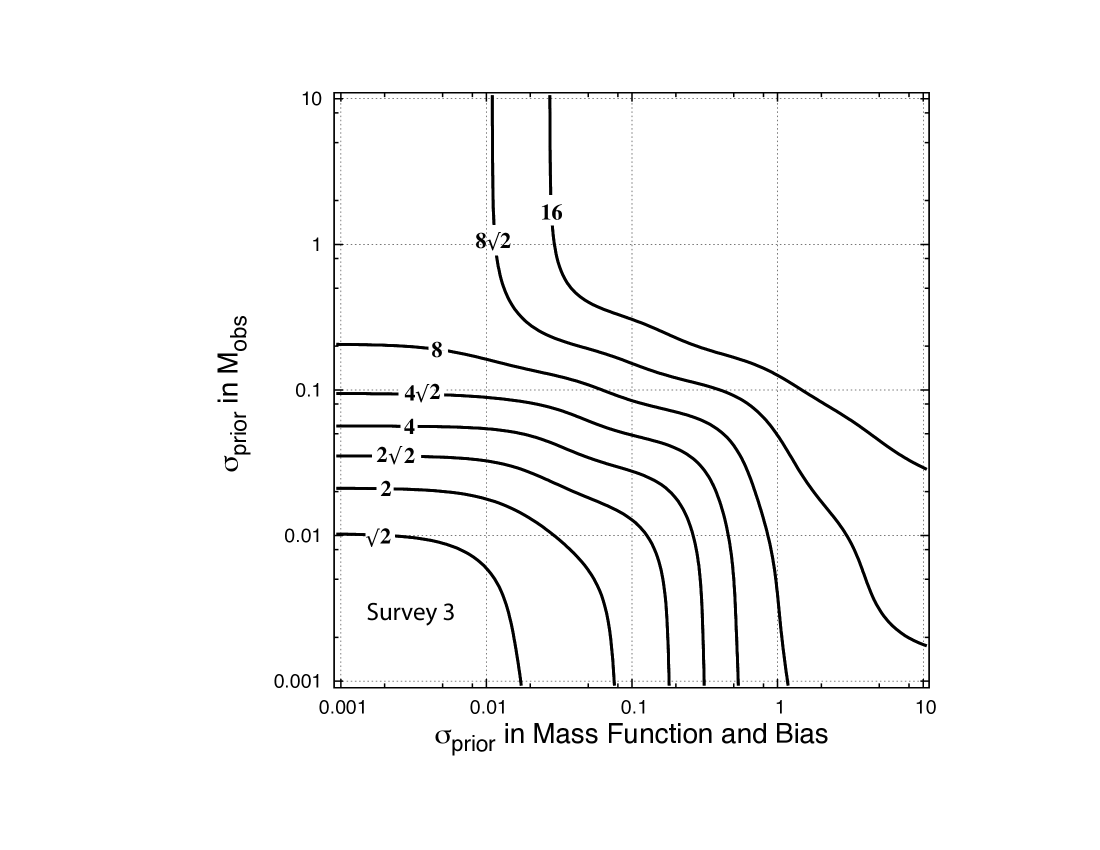
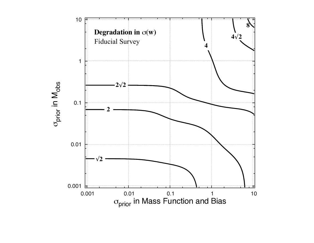
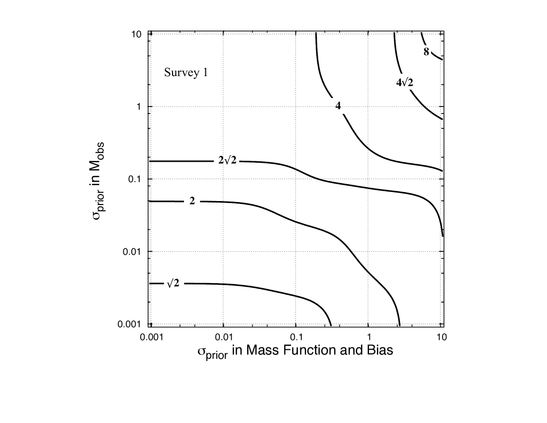
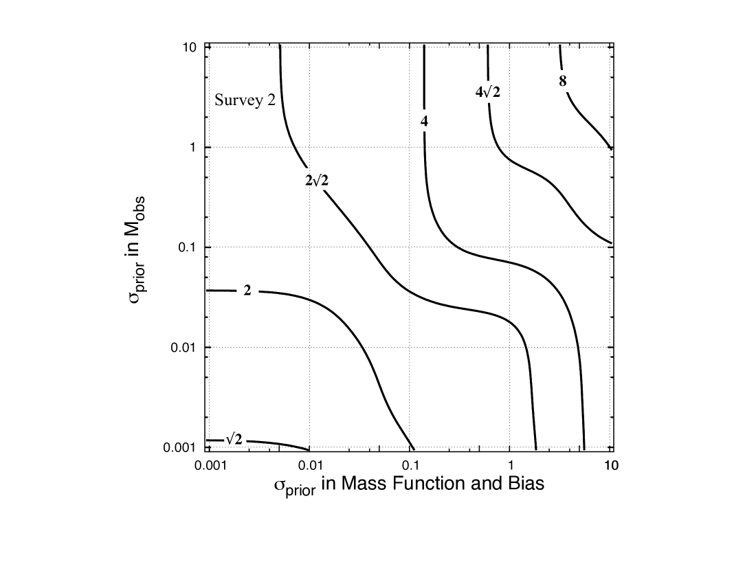
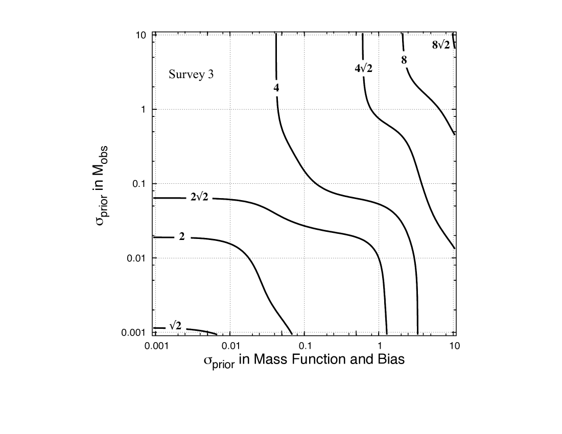
The contours in Figs. 2 and 3 display similar shapes. Contours tend to intersect the axes at right angles because of the very strong prior ($10^{-3}$) being imposed on one sub-space of parameters. The contour spacing gives the degradation in constraints as a function of prior on the complementary sub-space. For small systematic errors, the constraints on $\Omega_{\rm DE}$ and, especially, $w$ degrade faster in the $M_{\rm obs}$ direction than in the MF/B direction. Since the $M_{\rm obs}$ systematic degrees of freedom only have redshift, not mass, dependence, this indicates a larger sensitivity to redshift evolution, particularly in the case of $w$. For example, consider a $\sqrt{2}$ increase in $\sigma(w)$ for the default survey (upper-left panel of Fig. 3). For the case of perfect knowledge of the mass–observable priors, this degradation is reached when the mass function uncertainties are at the fractional level of $\sim 50\%$. Contrast this to the case of perfect knowledge of the mass function priors, for which a $\sqrt{2}$ increase in $\sigma(w)$ occurs with only $0.5\%$ error in the mass–observable parameters.

For the case of $\Omega_{\rm DE}$ shown in Fig. 2, the sensitivity to priors in $M_{\rm obs}$ and MF/B is more balanced for small values of $\sigma_{\rm prior}^{M_{\rm obs}}$ and $\sigma_{\rm prior}^{\rm MF/B}$. For the fiducial survey, errors of $\sim 0.1$ in the combined model parameters produce a factor 2 increase in $\sigma(\Omega_{\rm DE})$. For $\sigma_{\rm prior}^{M_{\rm obs}}\gtrsim 1.0$, the sensitivity of the degradation to priors on $M_{\rm obs}$ parameters decreases sharply. This plateau reflects the ability of mass function shape and clustering information alone to jointly calibrate $M_{\rm obs}$ parameters and $\Omega_{\rm DE}$ constraints. The same effect is noticeable in Fig. 3, though for $w$, the shape information provides the primary source of constraints of the $M_{\rm obs}$ parameters. When $\sigma_{\rm prior}^{\rm MF/B}$ is below the level of a few percent, the survey self-calibration is more effective at constraining the $M_{\rm obs}$ nuisance parameters, so that increasing $\sigma_{\rm prior}^{M_{\rm obs}}$ above $\sim 0.1$ does not result in further degradation of the cosmological constraints. The corresponding plateau in the MF/B parameter direction is much less pronounced. Consequently, if no prior information is available, mass-function/bias uncertainties dominate the error budget in cosmological parameters.

The contours of fixed degradation shift as one considers the other surveys shown in the remaining panels of Figs. 2 and 3. Comparing the right panels (showing surveys with $\sigma_{0}=0.5$), to the left (surveys with $\sigma_{0}=0.2$), we see that increasing the default $M_{\rm obs}$ scatter tends to shift the contours inwards, signifying an increase in sensitivity to the priors. This increase in sensitivity offsets the smaller baseline error in $\Omega_{\rm DE}$ and $w$, leading to roughly constant errors in these parameters for fixed nuisance priors. The shift inwards is most noticeable for large values of $\sigma_{\rm prior}$ for the surveys with $M_{\rm th}=10^{13.5}h^{-1}M_{\odot}$. In the limit of flat priors on both MF/B and $M_{\rm obs}$ parameters, we see from Table LABEL:tbl:constraints that the increase in scatter is beneficial for the surveys with $M_{\rm th}=10^{14.2}h^{-1}M_{\odot}$ but detrimental to the surveys with $M_{\rm th}=10^{13.5}h^{-1}M_{\odot}$. The former are dominated by shot noise, hence benefit from the increase in counts, but the latter are dominated by sample variance.

Comparing the bottom panels (surveys with $M_{\rm th}=10^{13.5}h^{-1}M_{\odot}$) with those above (surveys with $M_{\rm th}=10^{14.2}h^{-1}M_{\odot}$), we see that the overall effect of decreasing the mass threshold is to increase the sensitivity to MF/B and $M_{\rm obs}$ priors. Both $\Omega_{\rm DE}$ and w degradation contours shift inwards by as much as an order of magnitude. The effect is most pronounced in the MF/B direction. For the case of $w$ constraints with sharp $M_{\rm obs}$ priors, an intermediate plateau emerges in the range $\sigma_{\rm prior}^{\rm MF/B}\sim 0.1-1$. With lower $M_{\rm th}$, there is more information in cluster surveys, which requires very accurate priors to fully extract.

In summary, surveys with lower (better) baseline dark energy constraints have tighter requirements for priors on model systematic effects. For small $\sigma_{\rm prior}^{M_{\rm obs}}$ and $\sigma_{\rm prior}^{\rm MF/B}$ ($\lesssim 1$), the larger degradation for tighter baselines nearly offset, in the sense that the absolute uncertainties in $\Omega_{\rm DE}$ and $w$ at fixed $\sigma_{\rm prior}^{M_{\rm obs}}$ and $\sigma_{\rm prior}^{\rm MF/B}$ are almost constant among the surveys. For high $\sigma_{\rm prior}$ the better baseline does not compensate the more stringent prior requirement because the surveys with larger scatter are more sensitive to the prior uncertainties.

These results assume no mass-dependent evolution of the mass–observable relation. If we adopt the parameterization of Cunha (2009) which consists of adding one parameter to describe the mass-evolution of the bias and three parameters to characterize the mass-evolution of the scatter, we do not find significant qualitative changes. In survey 3, for example, assuming $\sigma_{\rm prior}^{\rm MF/B}=\sigma_{\rm prior}^{M_{\rm obs}}=0.1$ the four additional parameters yield essentially no shift in the contours. In other regions of the Figure, results can be more noticeable, with shifts in the $\sigma_{\rm prior}^{\rm MF/B}$ or $\sigma_{\rm prior}^{M_{\rm obs}}$ directions of up to a factor of 2. The rough shape of the curves is very similar. Degradations of $\sigma(w)$ are somewhat more sensitive to the inclusion of mass-dependent nuisance parameters. Assuming $\sigma_{\rm prior}^{\rm MF/B}=\sigma_{\rm prior}^{M_{\rm obs}}=0.1$ in Survey 3, addition of mass-dependence degrades constraints by roughly $\sqrt{2}$. The effects on the other surveys are even weaker since either they probe a smaller range in mass or they have smaller fiducial scatter.

Figure 4: Correlations between cosmological parameters and (top left) $M_{\rm obs}$ nuisance parameters, and (top right) MF/B nuisance parameters. The nuisance parameters not shown in each plot are fixed by infinitely sharp priors. Cosmological parameters, with the exception of $\Omega_{\rm DE}$ and w have $1\%$ priors and are not shown unless significant correlation with other parameters is present. The bottom plot shows the correlation between $M_{\rm obs}$, MF/B, $\Omega_{\rm DE}$, and w. We have added priors to all nuisance parameters such that $\sigma_{\rm prior}^{M_{\rm obs}}=\sigma_{\rm prior}^{\rm MF/B}=0.1$, which very roughly corresponds to our present knowledge of these parameters.

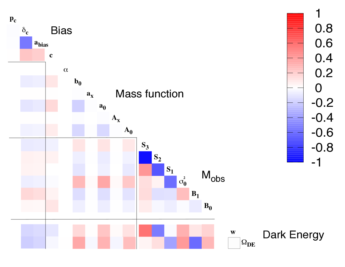
III.2 Parameter correlations

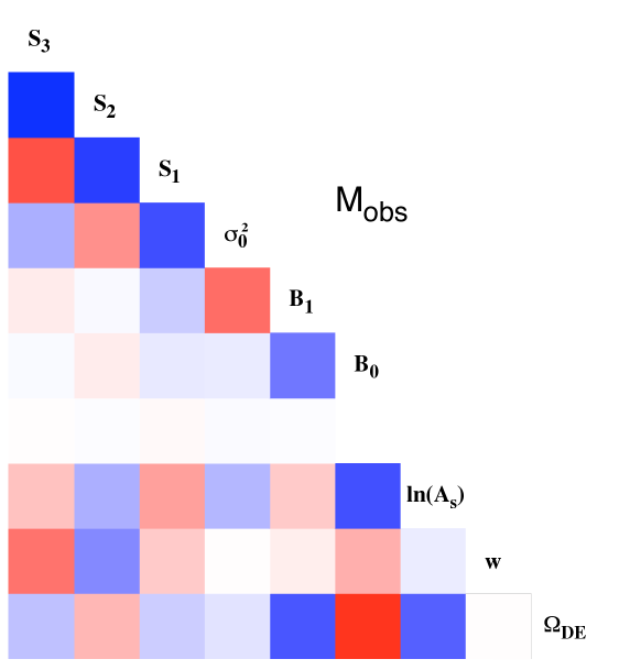
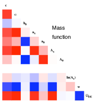
The halo modeling nuisance parameters have complex correlations among themselves and with the cosmological parameters. While one could imagine adopting a more orthogonal parameterization with potentially fewer parameters, the interpretation of the results would be hard to relate to the functional forms currently in use. Thus, we pursue the direct approach of exploring the Fisher correlations of the full parameter set. We begin by isolating the $M_{\rm obs}$ and the MF/B sub-spaces separately, using sharp priors on the complementary sub-space, then consider the full parameter covariance matrix under the assumption of a 10% prior uncertainty on the halo modeling parameters.

First, we add sharp priors to the MF/B nuisance parameters and consider the correlations between the $M_{\rm obs}$ nuisance parameters and the dark energy parameters, shown in Fig. 4 (top left). The labels of the $M_{\rm obs}$ and cosmological parameters occupy the diagonal of the correlation matrix. As described in Sec. II.4 the cosmological parameters other than $\Omega_{\rm DE}$ and $w$ have $1\%$ priors, and this level is small enough to remove almost all of their correlations with the other parameters. The exception is the normalization of the primordial power spectrum, $\ln(A_{s})$, which strongly correlates with $\Omega_{\rm DE}$ despite the $1\%$ prior.

From the plot, we see that the constant nuisance parameter of the mass bias ($B_{0}$) is strongly correlated with $\Omega_{\rm DE}$ whereas the redshift-related parameter ($B_{1}$) is markedly anti-correlated with $\Omega_{\rm DE}$. The variance nuisance parameters ($\sigma_{0}^{2}$, $S_{1}$, $S_{2}$, $S_{3}$) do not correlate as strongly with $\Omega_{\rm DE}$. In contrast, the equation of state $w$ is mostly correlated with the redshift-dependent variance parameters, and somewhat correlated to $B_{0}$. These correlations are consistent with the trends seen in Fig. 15 of Cunha (2009), showing the dependence of $\Omega_{\rm DE}$ and w constraints on the priors on different $M_{\rm obs}$ parameters.

On the (top right) plot of Fig. 4 we examine the correlations between the mass function nuisance parameters and the cosmological parameters. As in the above case, we apply infinitely sharp priors to all nuisance parameters not shown, and only plot the parameters with significant correlations. In this scenario, the $\ln(A_{s})$ correlates more weakly with all other parameters. The redshift-dependent parameters ($\alpha$, $a_{x}$, $A_{x}$) show strong positive correlations with $\Omega_{\rm DE}$, and strong negative correlations with $w$. The exponential cutoff parameter $c$ is also noticeably correlated with $w$ and $\Omega_{\rm DE}$. The redshift-dependent nuisance parameters are also strongly correlated among themselves, as are the constant parameters ($A_{0}$, $a_{0}$, and $b_{0}$), which are very weakly correlated with all other parameters.

In the bottom panel of Fig. 4, we investigate the full correlation matrix after imposing priors corresponding to $\sigma_{\rm prior}^{M_{\rm obs}}=\sigma_{\rm prior}^{\rm MF/B}=0.1$ to the $M_{\rm obs}$ and MF/B parameters (along with the $1\%$ cosmological priors). The $\ln(A_{s})$ correlations are very weak, hence, we do not show them. The choice of priors on the halo modeling parameters is admittedly crude, based roughly on the present-day understanding of the mass-function, bias, and the mass–observable relation. We caution that the correlations are a strong function of the imposed priors, so the chosen case is illustrative rather than definitive.

With these priors, the uncertainties in the $M_{\rm obs}$ nuisance parameters dominate the error budget in $\Omega_{\rm DE}$ and $w$. This result is consistent with the shape of the contours near $(0.1,\,0.1)$ in Figs. 2 and 3. Thus, the correlations between the $M_{\rm obs}$ and dark energy parameters are more pronounced, and, in general, resemble the correlations, performed under sharp MF/B priors, displayed in the top left panel. An exception is the correlation between the mass bias constant, $B_{0}$, and $\Omega_{\rm DE}$, for which the correlation in the full treatment is substantially weaker.

The mass function parameter correlations are substantially different from their isolated treatment. In particular, the redshift evolution parameters ($A_{x}$, $a_{x}$, and $\alpha$) largely disappear, and only the constant parameters ($A_{0}$, $a_{0}$ and $b_{0}$) contribute appreciably to the dark energy error budget. That this behavior differs from the isolated case is not too surprising. In the isolated case, the $M_{\rm obs}$ parameters are assumed to be perfectly known, so the only redshift evolution remaining in the model to compete with dark energy is contained in the MF/B parameters. In the full case, the assumed prior level of $M_{\rm obs}$ uncertainty is sufficient to dominate the evolutionary behavior, leaving the primary shape parameters of the MF as the means by which this sector affects dark energy constraints.

The full analysis also includes halo bias nuisance parameters. The parameters $\delta_{c}$ and $a_{\rm bias}$ strongly correlate with each other and also display weakly negative correlations with both $\Omega_{\rm DE}$ and $w$. The parameter $p_{c}$ is virtually uncorrelated with all the other parameters.

As we have mentioned before, the detailed behaviors are a consequence of the priors applied to the nuisance parameters. Had we used flat (very weak priors), the MF/B nuisance parameters would dominate the error budget, since self-calibration provides some constraints on the $M_{\rm obs}$ parameters. Then, the correlations of the mass function parameters between themselves and the cosmological parameters would more closely resemble those seen at the top right panel. The bias parameters would also exhibit somewhat stronger correlations.

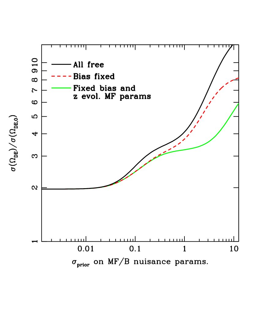
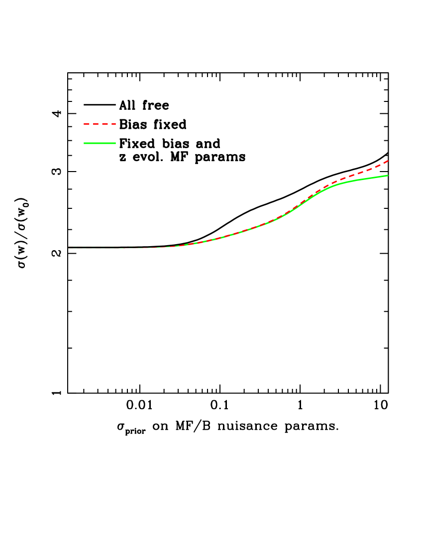
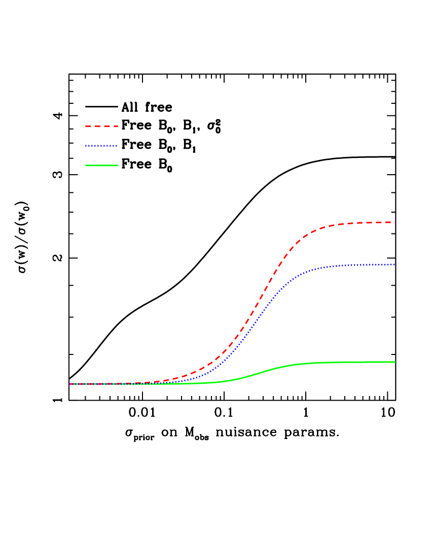
To further illustrate this sensitivity to priors on nuisance parameters, we explore the contributions of different sets of MF/B and $M_{\rm obs}$ nuisance parameters to degradations in $\sigma(\Omega_{\rm DE})$ and $\sigma(w)$. The top row of Fig. 5 shows the fractional degradation of $\sigma(\Omega_{\rm DE})$ and $\sigma(w)$ with respect to the baseline of the fiducial survey for the cases where (1) all the MF/B parameters are allowed to vary, (2) only the MF parameters are free, and (3) only the redshift-independent MF parameters are free. As before, we fix the priors on $M_{\rm obs}$ parameters so that $\sigma_{\rm prior}^{M_{\rm obs}}=0.1$.

In the upper left plot of Fig. 5, we see that the redshift evolution MF nuisance parameters ($A_{x}$, $a_{x}$, and $\alpha$) dominate the degradation of $\sigma(\Omega_{\rm DE})$ for moderate to large error, $0.1\lesssim\sigma_{\rm prior}^{\rm MF/B}\lesssim 1$. Below $\sigma_{\rm prior}^{\rm MF/B}\sim 0.1$, the constant MF parameters ($A_{0}$, $a_{0}$, $b_{o}$ and $c$) are the most relevant. The bias parameters are relevant in the high-uncertainty range, $1\lesssim\sigma_{\rm prior}^{\rm MF/B}\lesssim 10$. When $\sigma_{\rm prior}^{\rm MF/B}=0.1$, the parameters not related to redshift evolution, i.e., $A_{0}$, $a_{0}$, and $b_{0}$ dominate, as seen in Fig. 4. In the upper right plot, the constant MF nuisance parameters dominate the $w$ constraints up to $\sigma_{\rm prior}^{\rm MF/B}\sim 1$. For larger $\sigma_{\rm prior}^{\rm MF/B}$, the redshift evolution parameters become more important. The bias parameters are moderately relevant in the range $\sigma_{\rm prior}^{\rm MF/B}\sim 0.03-1$.

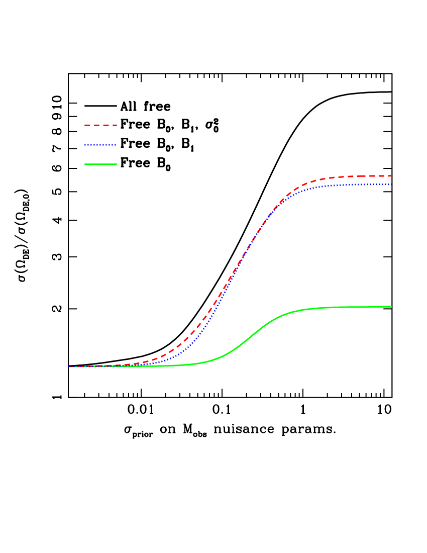
The bottom row of Fig. 5 shows the degradation of $\Omega_{\rm DE}$ and $w$ constraints as we vary priors on $M_{\rm obs}$ parameters while keeping $\sigma_{\rm prior}^{\rm MF/B}$ fixed at 0.1. From the lower left plot, we see that the parameters related to the redshift evolution of the mass–observable relation are the most important for virtually the entire interval we examine. In particular, the redshift evolution of the mass bias is the most relevant for $\Omega_{\rm DE}$ constraints. In the lower right plot we see that the redshift evolution of the mass variance dominates $w$ constraints for small uncertainties in the priors. For $\sigma_{\rm prior}^{M_{\rm obs}}\gtrsim 0.1$, the constant part of the variance, $\sigma_{0}^{2}$, as well as the redshift evolution of the bias, dominate. Constraints are almost independent of priors on the constant bias term, $B_{0}$, but this term does affect the power spectrum normalization, $\ln(A_{s})$.

Figure 5: Degradation of constraints on (left) $\Omega_{DE}$ and (right) equation of state $w$ as a function of the prior on the uncertainty in MF/B and $M_{\rm obs}$ nuisance parameters: $\sigma_{\rm prior}^{\rm MF/B}$ and $\sigma_{\rm prior}^{M_{\rm obs}}$, respectively (defined in Eqs. 21 and 22). Plots in the top row assume prior uncertainty on the $M_{\rm obs}$ parameters of $\sigma_{\rm prior}^{M_{\rm obs}}=0.1$. The solid black lines assume no priors on any of the MF/B nuisance parameters. The dashed red lines assume sharp priors on the three bias parameters, and the solid green lines assume sharp priors on the redshift evolution mass function nuisance parameters ($A_{x}$, $a_{x}$, and $\alpha$). In the range of $\sigma_{\rm prior}^{\rm MF/B}$ plotted, the green line is unaffected if priors are applied to the bias parameters or not. Plots in the bottom row assume prior uncertainty on the MF/B parameters of $\sigma_{\rm prior}^{M_{\rm obs}}=0.1$. The solid black lines assume no priors on any of the $M_{\rm obs}$ nuisance parameters. The dashed red lines assume sharp priors on the three parameters describing the redshift evolution of the mass variance. The dotted blue lines assume sharp priors on all four mass variance nuisance parameters ($\sigma_{0}^{2}$, $S_{1}$, $S_{2}$, and $S_{3}$), and the solid green lines assume sharp priors on all $M_{\rm obs}$ nuisance parameters except the constant bias term $B_{0}$.

IV Discussion

The results presented in this paper make a variety of assumptions of various degrees of relevance, which must be interpreted with caution. In this section we discuss the generality of some of our assumptions.

Parameterization of the mass–observable relation We parameterized the redshift evolution of the variance in $M_{\rm obs}$ using a cubic polynomial. Lima $\&$ Hu (2005) Lima and Hu (2005) show that the cubic polynomial is almost as complete a description as having fully independent scatter in $\sim 20$ redshift bins. Hence, we feel that our parameterization is conservative with regards to redshift evolution. There is no physical motivation for this choice, however, and if simpler parameterizations describe the data well, then constraints would improve - and the sensitivity to the uncertainty in the $M_{\rm obs}$ parameters would decrease. As a test, we eliminated the quadratic and cubic terms in the scatter in $M_{\rm obs}$. The contour lines of Figs. 2 and 3 shifted upwards by as much as factors of 5 in $\sigma_{\rm prior}$.

We did not include mass evolution of the mass–observable relation since evidence supporting this assumption from observations and simulations is currently weak. For surveys with high $M_{\rm th}$, we have checked that cosmological constraints are virtually unaffected by adding a cubic evolution of the mass scatter plus a linear evolution of the mass bias. For surveys with low $M_{\rm th}$, the mass terms cause an increase in sensitivity to both $M_{\rm obs}$ and MF/B parameters, which results in a shifting of the contours of Figs. 2 and 3 inwards. The additional $M_{\rm obs}$ nuisance parameters correlate strongly with the MF/B nuisance parameters, so that the sensitivity of both sets of parameters to the priors vary in similar fashion.

Our results are based on a quite generic procedure for adding priors. We did not strive for optimal dark energy constraints, or to accurately reproduce what specific observations and simulations might return. Understanding the optimal priors needed - for fixed observational/simulational costs - can be very valuable Wu et al. (2009), and such detailed studies are important complements to the generic treatment presented here.

As mentioned previously, we did not consider variations in w in this paper. The sensitivity of the Dark Energy constraints to the redshift-dependent nuisance parameters should increase, though it is not obvious that the relative importance of the $M_{\rm obs}$ and MF/B nuisance parameters would change significantly. The subject of cluster constraints on time-varying w, parameterized as $w_{0}$/$w_{a}$, is addressed in papers such as Wu et al. Wu et al. (2009) and Cunha et al Cunha et al. (2009).

V Conclusions

We investigate the sensitivity of dark energy constraints from clusters of galaxies to halo modeling uncertainties in the mass function, clustering bias, and the mass–observable relation. We find that mass–observable uncertainties dominate the error budget for both $\Omega_{\rm DE}$ and $w$ constraints for surveys with higher mass-thresholds, such as SZ surveys, assuming prior uncertainties of order $0.1$ on both mass–observable and mass-function/bias (MF/B) nuisance parameters. For surveys with lower mass-thresholds, the uncertainties in the mass–observable and MF/B nuisance parameters are more comparable, depending on the degree of prior knowledge assumed.

The variations in the sensitivity to the prior uncertainties are offset by the different baseline constraints of each survey. Not surprisingly, surveys with lower (better) baseline constraints have tighter requirements for priors on model systematic effects.

We examine the correlations between the nuisance and cosmological parameters for the fiducial survey for several different assumptions about prior knowledge of the nuisance parameters. If the mass–observable relation is perfectly known, the mass function parameters show strong positive (negative) correlations with $\Omega_{\rm DE}$ and w. If the mass function parameters are known to $\sim 0.1$, then $\sigma(\Omega_{\rm DE})$ and $\sigma(w)$ are dominated by the constant parameters of the mass function ($A_{0}$, $a_{0}$, and $b_{0}$). When the mass-function is held fixed, $\Omega_{\rm DE}$ is most sensitive to the normalization (bias) of the mass–observable relation and its redshift evolution, whereas $w$ is more sensitive to the redshift evolution of the variance.

We only consider individually self-calibrated cluster surveys. But as Cunha (2009); Cunha et al. (2009) show, cross-calibration is a powerful tool to improve knowledge of the mass–observable nuisance parameters and thereby tighten cosmological constraints. Strategies to optimize follow-up observations of cluster samples Wu et al. (2009) are relevant in this regard. The effects of using cross-calibrated cluster surveys would be to decrease the sensitivity to the mass–observable parameters, thereby increasing the relative sensitivity to the MF/B parameters. Our results adopted a specific parameterization of the mass function based on the assumption of collisionless dynamics of dark matter, with no gas physics. Baryonic effects can be large on the scale of clusters Stanek et al. (2009), and simulations exploring a broader range of baryon physics behavior are needed to ensure that the uncertainties in the mass function do not play a more significant role in limiting our knowledge of dark energy.

In conclusion, our results further illuminate challenges to precision cosmology with galaxy clusters. Observers and simulators should focus on characterizing the form of the mass–observable relation, since having the correct parameterization is essential to avoid biases in derived cosmological constraints. While we find that a mass function accuracy of about $10\%$ is a sub-dominant source of degradation of cosmological constraints, it still contributes measurably, particularly for surveys where significant cross-calibration or targeted follow-up will be possible.