Lower bounds on photometric redshift errors
from Type Ia supernovae templates

Abstract

Cosmology with Type Ia supernovae heretofore has required extensive spectroscopic follow-up to establish a redshift. Though tolerable at the present discovery rate, the next generation of ground-based all-sky survey instruments will render this approach unsustainable. Photometry-based redshift determination is a viable alternative, but introduces non-negligible errors that ultimately degrade the ability to discriminate between competing cosmologies. We present a strictly template-based photometric redshift estimator and compute redshift reconstruction errors in the presence of photometry and statistical errors. With reasonable assumptions for a cadence and supernovae distribution, these redshift errors are combined with systematic errors and propagated using the Fisher matrix formalism to derive lower bounds on the joint errors in $\Omega_{w}$ and $\Omega_{w^{\prime}}$ relevant to the next generation of ground-based all-sky survey.

1 Introduction

Accumulating evidence for an accelerating universe (Riess et al., 1998; Perlmutter et al., 1999; Astier et al., 2006; Wood-Vasey et al., 2007) is premised on the photometry of several hundred Type Ia supernovae whose redshifts were exquisitely determined through lengthy spectroscopic follow-up. At the current supernovae Type Ia discovery rate this situation remains manageable and spectroscopic follow-up continues to be the norm. Nonetheless, we are approaching an era of ground-based survey telescopes which may entail the discovery of a million or more of Type Ia supernovae per year of operation. This fantastic rate precludes spectroscopic follow up on all but the smallest fraction.

Errors from spectroscopically determined redshifts ($\pm$ 0.001) are typically much smaller than the errors associated with other parameters used in constructing the Hubble diagram (e.g., stretch and magnitude) and are justifiably neglected. As future survey instruments may discover thousands of Type Ia supernovae every night, a different method for ascertaining redshifts certainly must be employed. Photometric redshifts can be acquired much more expeditiously than their spectroscopic counterparts (the latter typically requiring numerous hours of dedicated time on a follow-up telescope). Unfortunately, all such alternative methods introduce non-negligible redshift error which must be accounted for in subsequent analyses.

Fortuitously, both of the long-standing photometric redshift techniques developed for galactic astronomy can be brought to bear on assessing the photometric redshifts of Type Ia supernovae. As the field of galactic redshift determination continues to mature, two competing techniques have emerged. The first technique is based on empirical fits derived from a training set having well established redshifts (Connolly et al., 1995). Recently, an empirical photometric estimator has been derived and applied to Type Ia supernovae (Wang, 2007). With this technique, magnitudes derived from fluxes in the grz bands are linearly combined to give a first-order redshift estimate. An improved redshift estimate is obtained by adding a stretch-like correction involving a ratio of the i band fluxes at peak and at 15 days in the supernovae rest frame. The coefficients are derived from a SNLS training set of 40 Type Ia supernovae. A dispersion ranging 0.031 to 0.050 is reported depending on the size of the training set. These comparatively large numbers are attributed to the photometric quality of the SNLS data and minimal statistics. In a follow up paper (Wang et al., 2007) it was shown that a dispersion of 0.005 may be achievable from supernovae with S/N $>$ 25, albeit supernovae that are temporally well sampled and free of obscuration from dust. A second technique involves broad band photometry acquired over multiple bands that is compared to predictions from galaxy spectral energy distributions (SEDs) to determine the redshift (Loh & Spillar, 1986) (and recently improved in (Bolzonella & Pelló, 2000)). The photometric error from either approach can be of order $\pm$ 0.1, which is generally unacceptable for the study of individual galaxies of galaxy clusters though is less problematic when performing statistical analyses of large data sets.

In this paper we adopt the latter approach to obtain photometric redshifts from template fitting. The advantage of this approach is that it obviates the need for an empirical model. However, a faithful Type Ia template is required. The requirement of a faithful supernova template is non-trivial since no two supernovae have identical spectra, the spectra evolve with time and further exhibit variation in luminosity. Further, Type Ia supernovae have no Hydrogen features in their spectra and hence lack the Lyman-break used for determining galactic redshifts. For template builders temporal evolution implies more work, for photometric redshift estimation purposes it is a boon: in essence each observing epoch permits an independent redshift determination. Furthermore, all epochs for which there is photometric data can be combined to jointly constrain the redshift. The redshift error which results when the template approach is applied to Type Ia supernovae is the main objective of this paper.

In Section 2 we describe the redshift error estimation methodology based on an archetypal Type Ia supernovae template set. In Section 3 we present results based solely on statistical error, then extend them to include systematic error derived from a distinct template set. From these combined statistical and systematic errors we derive ($\Omega_{w}$,$\Omega_{w^{\prime}}$) error ellipses based on a realistic supernovae distribution and idealized cadence. We conclude in Section 5 with a discussion of the implications of our work and discuss future extensions.

2 Methodology

The template fitting method begins with a Type Ia supernova template set. This set, typically generated in the supernovae rest frame, is modified to mimic the effects of redshift (the modified template set is henceforth referred to as the model set). Broad band filters are applied to spectra at various epochs in the model set to generate light curves. The light curve of a supernova whose redshift is to be determined (the reference supernova) is then compared to the light curves of the model set over a suitable redshift interval. The redshift of the light curve from the model set that most closely matches the light curve of the reference supernova (using a $\chi^{2}$ figure of merit) is assigned to the latter.

We adopt Nugent’s Type Ia branch normal templates (Nugent et al., 2002) for our studies. These templates span the temporal range from -16 day prior to +70 days after peak V magnitude (for a total of 87 epochs. Fluxes for epochs -20 through -17 are set to zero in the Nugent template set). The wavelength coverage is 1000 to 25000 Å binned into 2400 10 Å intervals. This set of 87 spectra constitutes the rest frame template set. There are four operations that must be applied to this template set to generate the model set (representing supernovae spectra at various redshifts in an expanding universe). The first two each involve a reduction in the flux by a factor of $(1+z)$, where $z$ runs from 0 to 1.0 in redshift intervals of 0.001, to account for time dilation and cosmological expansion (photon redshift) (Weinberg, 1972). A third is a time dilation factor of $(1+z)$ applied to each epoch (Goldhaber et al., 1996). The fourth involves redshifting the spectrum by $(1+z)$.

Our procedure then begins with Nugent’s Type Ia branch normal template set, where the interval of 1 day between successive epochs in the supernova rest frame is replaced by a separation of $(1+z)$ days in the frame of the observer. Two factors of $(1+z)$ factors were applied to the LSST bandpasses(Ivezić, 2007), which incorporate sky and filter transmission and CCD efficiency. Bandpass fluxes were derived by convolving the $ugrizy$ LSST filter set with the Nugent templates, after the templates were calibrated using a Johnson B band filter. Specifically, the Johnson $B$ filter was convolved with the Nugent template at time of peak epoch. The correction required to make the resulting $B$ passband magnitude equal to -19.3 was then applied to all subsequent data. The result of this exercise is the creation of 1001 light curve files, each containing the magnitudes for all 87 (time dilated) epochs in all six filters. This collection comprises the model set.

A key aspect of our method involves the conversion of magnitudes into colors. As is well known, the relationship between luminosity and flux requires knowledge of the luminosity distance. However, the luminosity distance depends on the choice of cosmological models luminosities. As will be made more explicit below, the conversion from magnitudes to colors permits cancellation of the (unknown) luminosity distance.

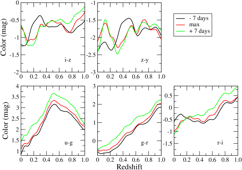
Each panel in Figure 1 shows the evolution of one the five LSST colors obtained by applying the four corrections described above to the LSST filter set convolved with Nugent’s model template set. Each color is shown as a function of redshift for three separate epochs. Over the epoch range shown in this figure the $g-r$ color exhibits nearly monotonic behavior and would be the most effective of the five colors over the depicted redshift interval in estimating redshifts. The actual reconstruction efficiency will be considerably more nuanced when multiple colors, multiple epochs and measurement noise are involved, as we shall see below.

Figure 1: (lower left to upper right) LSST u-g, g-r, r-i, i-z and z-y colors as a function of redshift at 7 days before maximum (black), at maximum (red) and 7 days after maximum light (green) for the Nugent template set.

From these colors we now proceed to define a measure of goodness of fit $chi^{2}(z)$ for the $u-g$ color as

$$\chi^{2}(z)=\sum_{i}^{epochs}((u(z)-g(z))-(u(z^{\prime})-g(z^{\prime})))_{i}^{2},$$ (1)

where $u(z)$ and $g(z)$ represent magnitudes in the $u$ and $g$ bandpasses from the reference set at redshift $z$ at epoch $i$ and $u(z^{\prime})$ and $g(z^{\prime})$ are defined similarly for the model set. The sum is over all $i$ epochs.This procedure is generalized in an obvious manner to include five colors ($u-g$, $g-r$, $r-i$, $i-z$ and $z-y$) that can be constructed from the six LSST bandpasses. Equation 1 makes explicit how luminosity distances cancel if one chooses to work with color magnitudes. The $\chi^{2}$ expression in Equation 1 is actually a 1001 element array, with each element of the array containing a $\chi^{2}$ value for a given combination of $(z,z^{\prime})$. The entire array is generated by fixing $z$ and varying $z^{\prime}$ over the interval 0$\ <z^{\prime}<\$1 in increments of 0.001. The minimum of this array corresponds to the light curve at z’ from the model set that most closely matches the redshift of the reference light curve at $z$. A perfect reconstruction results in $z=z^{\prime}$. Chi-squared values spanning the entire 1001 $\times$ 1001 $\{z,z^{\prime}\}$ space are generated by choosing reference light curves over the interval 0$\ <z<\$1 in increments of 0.001.

The $\chi^{2}(z)$ value reflects the degree of overlap between the light curve of a reference supernova located at redshift $z$ with respect to the light curves of model supernovae located at $z^{\prime}$. It bears emphasizing that the reference and model sets are both drawn from the same Nugent template set. The overlap that would result if spectral and variability were included undoubtedly would be less pronounced.

3 Results

Though the methodology described above is straightforward, it is instructive to explore a highly simplified model for the purposes of comparison with results from using the template spectra. An analytical expression for $\chi^{2}$ at an arbitrary redshift can be written down if filter transmission coefficients and spectral fluxes (at all epochs) are constant. The left panel in Figure 2 compares the results from an analytic model (dashed) with those from the methodology described in Section 2 (solid) for a reference supernova at a redshift 0.5. In both the analytical and numerical examples the LSST $u$ bandpass is used, however, the transmission coefficients have all been set to 1.0 over the rest frame interval 3190 $<\lambda<$ 4120 (those wavelength bins in the rest frame $u$ filter whose transmission coefficient exceeds 0.005). The redshifted filter is convolved with a toy spectrum whose rest frame fluxes are also set to 1.0 over all wavelengths and all epochs. Both the analytical and numerical examples are described by Equation 1, but here with $g(z)=g(z^{\prime})=0$. The close agreement between them benchmarks the numerical approach.

The black curve in the right hand panel of this same figure is the $\chi^{2}$ for the $u-g$ color as described by Equation 1, using the $u$ filter and toy spectrum as described above, and with a rest frame $g$ filter whose transmission coefficients are 1.0 over the region 3870 $<\lambda<$ 5610. The featureless toy model produces a $\chi^{2}$ curve whose values are non-zero only because the $u$ and $g$ bandpasses have different widths and are centered on different wavelengths. For comparison, the $\chi^{2}$ values for the $u-g$ color derived from the Nugent templates and LSST bandpasses are also displayed (red). Note that the $\chi^{2}$ curve derived from the templates is much steeper than the toy model and further displays structure which can be traced back, in principle, to various spectral features. In the absence of noise the reconstructed redshift corresponding to the $\chi^{2}$ minimum coincides with the reference redshift of 0.5. A more realistic example includes measurement noise. The green curve in the right panel of Figure 2 are the $\chi^{2}$ values for the $ug$ color derived from the templates where noise has been added to both the reference and model light curves drawn from a normal distribution with standard deviation of 0.05. As this curve illustrates, noise obscures the location of the true minimum in two ways: it increases bin-to-bin jitter and broadens the minimum. Both effects increase the probability that the location of the true minimum (located at $z^{\prime}$) will differ from the reconstructed minimum (located at $z$).

Figure 2: (Left) $\chi^{2}$ values (in units of flux) as function of redshift for a simplified analytical model (dashed) versus those derived from the numerical approach described in the text (solid) for a reference supernova at $z$ = 0.5. Small differences between the two approaches are attributed to binning of the latter, and the absence of noise the reconstructed redshift is 0.5 with either approach. (Right) $\chi^{2}$ values (in units of magnitudes) but for the LSST derived $u-g$ color with no noise (red), and with the addition of noise drawn from a normal distribution with $\sigma$ = 0.05 (green). For comparison purposes, the result of the toy model is again shown, but now for the $u-g$ color (black, also in units of magnitudes). It is noteworthy that $\chi^{2}$ is much steeper for the template than the toy model.

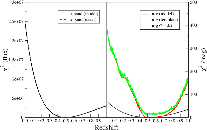
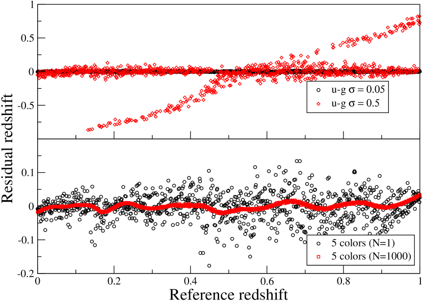
The solid curve in the right panel of Figure 2 is a single realization of Gaussian noise. To get a statistical measure of the effect that noise has on obscuring the location of the true minimum, Monte Carlo simulations consisting of 1000 random instances of photometric measurement noise were done for each redshift interval. From these runs the median redshift value was chosen and compared to the redshift of the reference light curve. The top panel in Figure 3 contains two curves, each a plot of the residual redshift versus the redshift of the reference light curve using LSST $u$ and $g$ bandpass filters. The residual redshift is defined here as $(z_{rec}-z)/z$, where $z_{rec}$ is the reconstructed redshift based on the above procedure and $z$ is the redshift of the reference light curve. The sole difference between the curves in the upper panel of Figure 3 is the amount of Gaussian noise added to the reference and model light curves. It is seen that reconstruction of the redshift is quite faithful for the addition of Gaussian noise sampled from a normal distribution with a $\sigma$ of 0.05, but erratic behavior is observed with a $\sigma$ of 0.5. The bifurcation one sees in this panel for large photometric errors is due to non-monotonic nature of color versus redshift curve in Figure 2 ($u-g$ panel). Since for z $>$ 0.2 (depending on epoch) the $u-g$ color function is double-valued, the $\chi^{2}$ minimization procedure alternates between two possible redshift solutions, giving rise to the aberrant behavior of the red curve in Figure 4. By this same logic from Figure 2 one can predict more rational behavior for $z\sim$ 0.5, which is in fact manifested in Figure 4.

As the lower panel demonstrates, the erratic behavior in the top panel can be modified using all five colors combinations of the LSST filter set. Though considerable bin-to-bin scatter is observed in the reconstructed redshift from only a single realization of Gaussian noise (circles), a 1000 realizations generates the smoothly varying curve (squares) in this same panel. Notably, the data are well-behaved with no catastrophic outliers even with the addition of considerable noise. As noted above, the observed undulations ultimately can be traced to template spectral features passing through the filter set.

Figure 3: (Top) Residual redshifts as defined in the text for a single realization of noise drawn from a normal distribution with $\sigma$ = 0.05 and 0.5 computed for the LSST $u-g$ color assuming a nightly observing cadence. (Bottom) Same, but for a single realization (circles) and the median of 1000 realizations (squares) of noise drawn from normal distribution with $\sigma$ = 0.5 for all five LSST colors.

The lower panel in Figure 4 shows the residual redshifts using all five bandpass colors at every epoch, but now with Gaussian noise drawn from a normal distribution with a $\sigma$ of 0.05. In this plot the residual redshifts are divided a factor of $(1+z)$.

Figure 4: (Bottom) The median of the residual redshifts of 1000 realizations drawn from a normal distribution with $\sigma$ = 0.05 for all five LSST colors and assuming a nightly observing cadence. (Top) Same, but assuming an observing cadence of every 5^th night (red), 20^th night (green) and 45^th night (blue) night. For reference the curve from the bottom panel is also included (black).

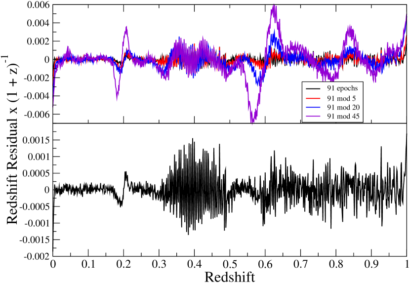
For this highly idealized cadence the standard deviation of the redshift residuals is 4.2$\cdot$10^-4 over the redshift interval 0 $\leq z\leq$ 1.0.

The redshift residuals presented so far have been constructed using all 87 epochs. It is certainly unrealistic for a survey instrument to sample any given supernovae on a nightly basis. The upper panel in this same figure shows residual redshift results for successively sparser sampling intervals. As a benchmark the black curve from the lower panel is included, along with the residuals for cadences representing observations using all six LSST filters every 5^th (red), 20^th (green) and 45^th (blue) night. The corresponding standard deviations are 5.2$\cdot$10^-4, 9.2$\cdot$10^-4 and 1.8$\cdot$10^-3, respectively. Clearly, there are redshift intervals for which even an extremely sparse cadence may provide an accurate photometric redshift estimate. In any case, the data can be corrected for the bias (departure from perfect reconstruction) seen in these figures. By contrast, errors associated with the redshift residuals cannot be compensated for. Figure 5 is a plot of the inverse square of the residual redshift errors for each of the five LSST colors assuming an observing cadence of every fifth epoch. In this plot larger values correspond to smaller errors and illustrates the ”effectiveness” of each color for getting accurate redshift in a given redshift range. This same plot also shows the total errors when all five colors are used (black curve). Note that even though $\sigma^{-2}$ is an additive quantity, the sum from each of the individual colors does not equal that from the combined five colors since the colors are not linearly independent. The effectiveness of the $z-y$ color is particularly striking. Specifically, a conceivable strategy could be to restrict photometry to the $z$ and $y$ filters over the redshift interval 0.15 $<z<$ 0.3 should the templates resemble actual supernovae spectra in these bandpasses.

Figure 5: The inverse square of the errors of the redshift residuals from 1000 realizations of noise from a normal distribution with $\sigma$ = 0.05 and a observing cadence of every 5^th night in each of the five LSST colors and the total inverse square error (black).

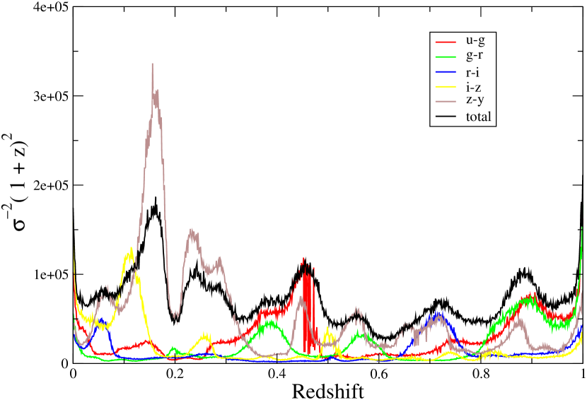
As an optimal supernovae cadence for LSST has yet to be adopted, subsequent analyses are based on the assumption that a particular supernova will be visited in each of the six filters every fifth night.

In addition to the statistical error arising from Poisson noise and imperfect sampling, there may be a plethora of systematic errors that will further degrade photometric redshift accuracy. One systematic error than is relevant here concerns choice of templates. To generate binned systematic errors we chose a second model template set constructed by (Hsiao et al., 2007). This set has identical spectral coverage as the Nugent set, but epoch coverage is extended to +85 days (for this purpose epochs beyond day 70 are ignored). We derive systematic errors by again computing the standard deviation in the redshift residuals for 1000 trails sampling from a normal distribution with $\sigma=0.05$ and also very fifth night, but now using this second model set. The standard deviations that result are taken to be systematic error due to imperfect knowledge of the template set.

4 Cosmological Parameters

Ultimately, one wishes to transform the redshift errors arising from the imperfect photometric redshift reconstruction onto the accuracy with which one can determine cosmological parameters. A common approach for propagating redshift errors from data, or estimated errors from future data sets, is via the Fisher matrix. The Fisher matrix is a statistic which combines data errors with model sensitivities and whose inverse is the covariance matrix. Several techniques have been proposed for propagating redshift error using the Fisher matrix formalism; here we employ the method advanced by (Huterer et al., 2004). In their approach an $N\times N$ Fisher matrix (representing $N$ cosmological parameters) is expanded by $M$ rows and columns representing the $M$ supernovae whose redshift errors are to be marginalized over. The off-diagonal terms in these $M$ rows and columns contain cross products of the derivatives of the distance modulus $\mu$ with respect to redshift times the derivatives of the distance modulus with respect to $\Omega_{M}$ or $\Omega_{\Lambda}$, e.g., $\partial\mu/\partial z\cdot\partial\mu/\partial\Omega_{M}$. The $M$ diagonal terms contain inner products of the form $\partial\mu/\partial z\cdot\partial\mu/\partial z$ and all $M\times M$ terms are evaluated at the (binned) supernova redshift and weighted by the binned errors. When constructing the quantity $\partial\mu/\partial z$ the definition of $\mu$ is expanded to include stretch (but not derivatives of the $K$-corrections as was required in (Huterer et al., 2004) as we are working with magnitudes derived directly from the spectra, not the light curves). As a cross check this discrete method was compared with an analytical Gaussian distribution proposed by (Tegmark et al., 1998). The upper panel in Figure 6 compares the exact result with the binned approach for a Gaussian distribution of 100 supernovae at an average redshift of $z$ of 0.55, with a standard deviation of 0.2 and each with a magnitude error of 0.5 for a flat, matter-filled universe ($\Omega_{M}$=1, $\Omega_{\Lambda}$=0).

Figure 6: (Top) Error ellipses in the {$\Omega_{M}$,$\Omega_{\Lambda}$} plane from Fisher matrices derived from an analytical (solid) and discrete model (dashed) of the Gaussian supernovae distribution as described in the text. In both cases a flat, matter-filled universe ($\Omega_{M}$ = 1, $\Omega_{\Lambda}$ = 0) was assumed. (Bottom) Same, but now in the {$\Omega_{w}$, $\Omega_{w^{\prime}}$} plane and assuming the standard cosmology ($\Omega_{M}$ = 0.3, $\Omega_{\Lambda}$ = 0.7). A series of five error ellipses are shown, with the blue ellipse representing the addition of a generic systematic error with a $\sigma_{sys}$ of 0.0002. The violet ellipse represents the addition of systematic error derived from utilizing a distinct model template set (see text). The aquamarine ellipse represents a generic systematic error with a $\sigma_{sys}$ of 0.02 as in (Huterer et al., 2004; Zhan et al., 2008). In all three cases the systematic error is added in quadrature to the redshift errors described by the plot in the lower panel of Figure 4 for the supernovae distribution described in (Zhan et al., 2008). The inset shows on an expanded scale the three smallest error ellipses from the main panel representing pure photometry error (black), photometry and redshift errors (red). The blue ellipse is included in the inset for comparison.

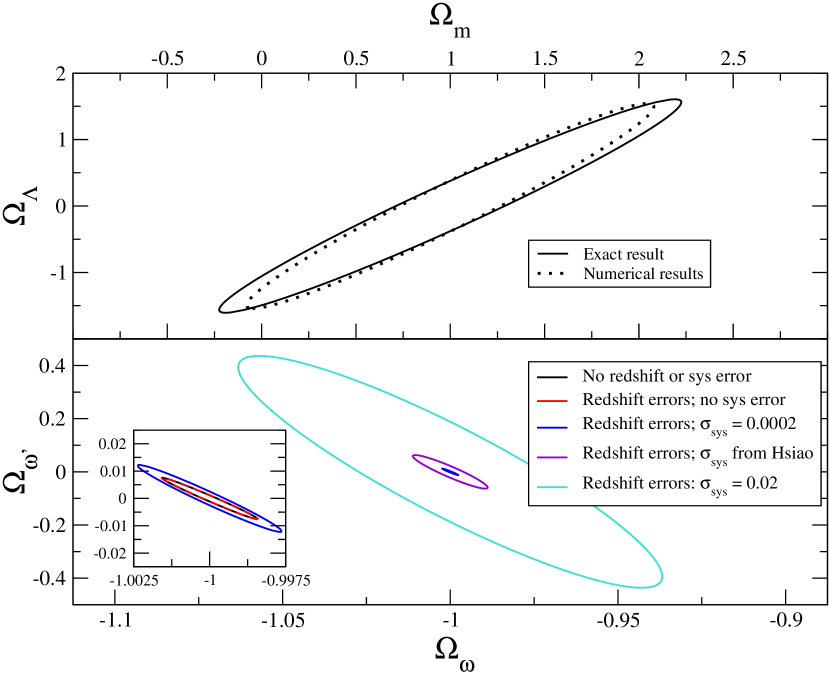
The variation between the two approaches is ascribed to the discrete binning (16 bins) that all but disappears as the number of bins approaches 100 (at the expense of computational resources required to invert a 102 $\times$ 102 matrix).

A survey instrument like LSST with an étendue of 220 m²deg² will cover the entire sky every few nights in each of its six filters. Though its primary cadence may not be optimal for detection and follow up of Type Ia supernovae, LSST is nevertheless expected to discover several million Type Ia supernova in the course of its 10 year mission. This sheer number of supernovae will allow unprecedented examination of systematics related to reddening, host contamination, evolution and other effects that interfere with a precise determination of the distance modulus. Lacking a formal supernovae cadence for LSST we adopt the estimated number of supernovae per steradian per unit redshift per year in the observer frame as derived by (Zhan et al., 2008).

The ellipses in the lower panel in Figure 6 are derived from combined photometry, photometric redshift and systematic errors. Photometry errors ($\sigma_{p}$ = 0.17) and photometric redshift errors associated with the orange curve from the upper panel in Figure 5 ($\sigma$ = 0.05; every 5^th epoch) are first reduced by the number of supernovae in each of the rebinned redshift bins (16 equally spaced bins spanning 0 $<z<1.6$; weights for $z>$ 1.0 were made large to effectively limit the analysis to $0<z<1.0$). Systematic error derived in the manner described above was likewise rebinned and added in quadrature to the photometry and photometric redshift error. A 2 $\times$ 2 Fisher matrix representing the cosmological parameters $\Omega_{w}$ and $\Omega_{w}^{\prime}$ was expanded to an 18 $\times$ 18 matrix to accommodate these binned errors. This matrix was inverted and marginalized along the 16 rows and columns representing the binned errors. The resultant 2 $\times$ 2 inverse matrix was again inverted to generate the purple ellipse in the lower panel of Figure 6. Several related error ellipses are shown in this same panel for comparison purposes. Photometry error alone produces the black ellipse - addition in quadrature with photometric redshift errors produce an ellipse (red) that is indistinguishable from the black ellipse (see inset). This behavior, also noted by (Huterer et al., 2004), is due to the particular choice of photometry error and will evolve as photometry errors become more stringent. The blue ellipse demonstrates that systematic errors have no tangible effect until it reaches a level that coincides with the level of systematic error derived from the Hsiao template set ($\sigma_{sys}\sim$ 0.003). The largest ellipse (aquamarine) assumes a $\sigma_{sys}$ of 0.02 in keeping with assumptions made by (Huterer et al., 2004; Zhan et al., 2008).

5 Discussion

A new era of large aperture ground-based survey telescopes is driving the need for an alternative to costly spectroscopic follow up to obtain Type Ia supernovae redshifts. In this paper we apply a technique that utilizes templates to derive these redshifts photometrically based on a $\chi^{2}$ minimization procedure. Though applied to proposed LSST bandpasses, this approach is broadly applicable to any instrument acquiring photometric data. Limited Poisson statistics, observational and instrumental noise are modeled by the addition of Gaussian noise. Further, we approximate a realistic supernovae campaign cadence by restricting the number of epochs used to construct our $\chi^{2}$ figure of merit whose minimum is assigned to the redshift of the reference supernova. Multiple realizations of these simulations generate the statistics from which we extract the residuals and their standard deviations for each redshift bin. Ultimately, of course, we are interested in the implications for cosmology with redshifts derived in this manner. To proceed, we overlay a realistic redshift distribution broken into observing bins. These redshift errors are then placed in a matrix along with the weights of the cosmological parameters of interest, with a common multiplier reflecting photometry errors. Both the redshift errors and photometry errors are weighted by the number of supernovae per bin; binned systematic errors derived from a distinct model set are added in quadrature but are not weighted by the number of supernovae per bin. The resulting Fisher matrix generates error ellipses in the $\Omega_{\Lambda}$ and $\Omega_{M}$ and $\Omega_{w}$ and $\Omega_{w^{\prime}}$ planes.

Though considerable work has been done to ascertain the feasibility of weak-lensing measurements from ground-based instruments (Wittman, 2005; Jain et al., 2006; Asztalos et al., 2007), comparatively little has been done regarding Type Ia supernovae. This work is the first to put all the major elements together to ascertain the relevance of supernovae cosmology from ground-based instruments. In particular, it establishes a minimal redshift error that can be expected from photometric redshift determination. The error ellipse derived in Figure 6 from plausible photometric redshift and systematic errors is considerably more constrained than would be the case if one assumed constant photometric redshift and systematic errors of magnitude 0.02 that have appeared in the literature (Huterer et al., 2004; Zhan et al., 2008). A corollary is that should systematic error ultimately be controllable to $\sim$ 0.003, then photometric redshifts would be very effective at discriminating between many competing cosmologies.

A more realistic observing cadence, Type Ia supernovae distribution and noise models are readily incorporated into this framework. Indeed, though the scope of this work has been strictly limited to template models, it is readily modified to actual supernovae spectra. Progress is being made extending this work to include simulated cadences and actual Type Ia supernovae spectra and work continues on improved noise models. Extensions of this work must further address covariances among the techniques used for typing, epoch and redshift assignments.

We conclude with a final observation. At present this method is limited to stretch $\sim$ 1 supernovae since, at present, there is no firm consensus as to the underlying mechanism for stretch. However, correlations between various spectral features and stretch are well established (Nugent et al., 1995; Wagers et al., 2009) and with these correlations in hand we have embarked on the construction of Type Ia supernovae templates with stretch different from one. With these templates in hand the above technique could be extended by simply the addition of a loop over templates. One advantage to templates constructed in this manner is that the variability would not necessarily be restricted to that observed in actual Type Ia supernovae (Guy et al., 2007).

References

- Riess et al. (1998) Riess, A. G., et al. 1998, AJ, 116, 1009
- Perlmutter et al. (1999) Perlmutter, S., et al. 1999, ApJ, 517, 565
- Astier et al. (2006) Astier, P., et al. 2006, A&A, 447, 31
- Wood-Vasey et al. (2007) Wood-Vasey, W. M., et al. 2007, ApJ, 666, 694
- Connolly et al. (1995) Connolly, A. J., Csabai, I., Szalay, A. S., Koo, D. C., Kron, R. G., & Munn, J. A. 1995, AJ, 110, 2655
- Loh & Spillar (1986) Loh, E. D., & Spillar, E. J. 1986, ApJ, 303, 154
- Bolzonella & Pelló (2000) Bolzonella, M., & Pelló, R. 2000, Clustering at High Redshift, 200, 392
- Wang (2007) Wang, Y. 2007, ApJ, 654, L123
- Wang et al. (2007) Wang, Y., Narayan, G., & Wood-Vasey, M. 2007, MNRAS, 382, 377
- Nugent et al. (2002) Nugent, P., Kim, A., & Perlmutter, S. 2002, PASP, 114, 803
- (11) ww.phy.bnl.gov/p̃artsem/fy07/BNL_Wood-Vasey_20070719.key/droppedImage-8.pdf
- Weinberg (1972) Weinberg, S. 1972, Gravitation and Cosmology: Principles and Applications of the General Theory of Relativity, by Steven Weinberg, pp. 688. ISBN 0-471-92567-5. Wiley-VCH, July 1972
- Goldhaber et al. (1996) Goldhaber, G., et al. 1996, Nuclear Physics B Proceedings Supplements, Vol. 51, 51, 123
- Ivezić (2007) Ivezić, Ž. 2007, Why Galaxies Care About AGB Stars: Their Importance as Actors and Probes, 378, 485
- Hsiao et al. (2007) Hsiao, E. Y., Conley, A., Howell, D. A., Sullivan, M., Pritchet, C. J., Carlberg, R. G., Nugent, P. E., & Phillips, M. M. 2007, ApJ, 663, 1187
- Huterer et al. (2004) Huterer, D., Kim, A., Krauss, L. M., & Broderick, T. 2004, ApJ, 615, 595
- Tegmark et al. (1998) Tegmark, M., Eisenstein, D. J., & Hu, W. 1998, arXiv:astro-ph/9804168
- Zhan et al. (2008) Zhan, H., Wang, L., Pinto, P., & Tyson, J. A. 2008, ApJ, 675, L1
- Nugent et al. (1995) Nugent, P., Phillips, M., Baron, E., Branch, D., & Hauschildt, P. 1995, ApJ, 455, L147
- Wittman (2005) Wittman, D. 2005, ApJ, 632, L5
- Jain et al. (2006) Jain, B., Jarvis, M., & Bernstein, G. 2006, Journal of Cosmology and Astro-Particle Physics, 2, 1
- Asztalos et al. (2007) Asztalos, S., de Vries, W. H., Rosenberg, L. J., Treadway, T., Burke, D., Claver, C., Saha, A., & Puxley, P. 2007, ApJ, 659, 69
- Wagers et al. (2009) Wagers, A., Wang, L., Asztalos, S., Submitted to ApJ
- Guy et al. (2007) Guy, J., et al. 2007, A&A, 466, 11