Footprints of sticky motion in the phase space of higher dimensional nonintegrable conservative systems

Abstract

“Sticky” motion in mixed phase space of high dimensional conservative systems is difficult to detect and to characterize. Its effect on quasi-regular motion is quantified here with four different measures, related to the distribution of the finite time Lyapunov exponents. We study systematically conservative maps from the uncoupled two-dimensional case up to coupled maps of dimension $20$. We find sticky motion in all unstable directions above a threshold $K_{d}$ of the nonlinearity parameter $K$ for the high dimensional cases $d=10,20$. Moreover, as $K$ increases we can clearly identify the transition from quasiregular to totally chaotic motion which occurs simultaneously in all unstable directions. Results show that all four statistical measures sensitively probe sticky motion in high dimensional systems.

1 Introduction

The dynamics of conservative systems consists of different types of motion, from regular over quasi-regular to chaotic, depending on the perturbation parameter. Usually, in $d=2$ dimensional conservative systems regular islands (Kolmogorov-Arnold-Moser KAM tori) can break as the perturbation parameter increases, and chaotic trajectories may coexist with regular islands [1]. This regime is called quasiregular. Chaotic trajectories may be trapped around stable islands creating “sticky” motion (for a review see [2]). In such cases the dynamics in phase space can be very structured and the motion is non-ergodic. Analytical results for physical quantities in the quasiregular regime are rare and it is very desirable to obtain tools which quantify degrees of ergodicity and hyperbolicity, as for example the angle between the stable and unstable manifolds obtained via the covariant Lyapunov vectors [3, 4]. Even for apparently totally chaotic systems, tiny regular islands may appear which induce sticky motion as exemplified in Fig. 1a with the phase space of the $d=2$ dimensional kicked rotor [Eqs. (3] for the nonlinearity parameter $K=5.79$. The dynamics looks totally chaotic – yet, tiny regular islands appear near the points $(x,p)\sim(4.6,2.9),(1.7,-2.9)$ (see boxes), if enough initial conditions are sampled. Such islands become visible with sufficient magnification (Figs. 1b-c).

Figure 1: Phase space for $K=5.79$. (b) and (c) are magnifications from the boxes shown in (a).

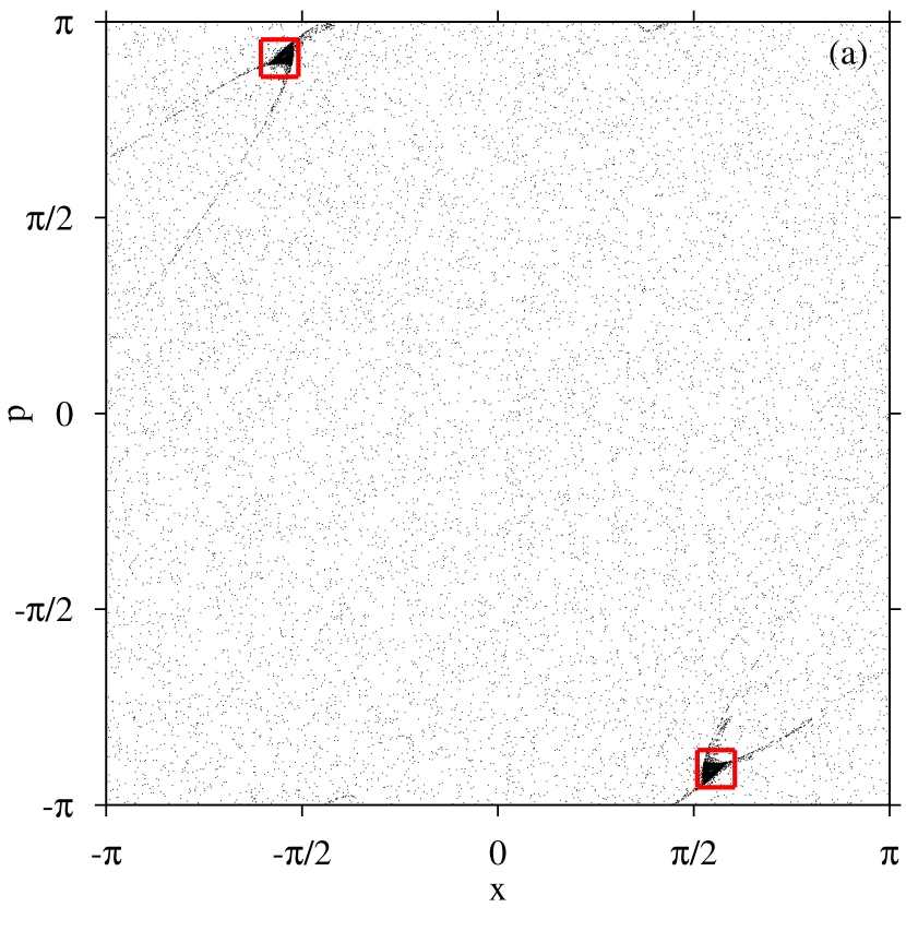
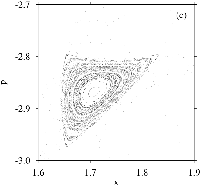
Hence, the question arises how these tiny regular islands can be identified with not more information than provided by Fig. 1a. In higher dimensions, the information equivalent to Fig. 1a must be cast in a different form since Poincaré Surfaces of Section (PSS) cannot be plotted. In fact, for $d>2$ dimensional conservative systems, due to Arnold diffusion, the KAM surfaces do not divide the whole phase space into a set of closed volumes. Although the effect of stickiness of $N$-dimensional invariant tori has been analyzed for the asymptotic decay of correlations and anomalous diffusion [5], to the best of our knowledge, the behavior of sticky trajectories in higher-dimensional systems has never been quantified and explored systematically.

In the following we present extensive numerical simulations to detect and quantify sticky motion in the phase space of quasiregular and chaotic conservative systems with up to 20 dimensions. To fulfill this task we analyze small changes in the finite time Lyapunov exponents (FTLE) distribution using four quantities: the variance $\sigma$, the skewness $\kappa_{3}$, the kurtosis $\kappa_{4}$ and ${\cal P}_{\Lambda}$, the normalized number of occurencies of the most probable finite time Lyapunov exponent. The first three quantities were analyzed in the two-dimensional standard map for the distribution of the finite time stability exponents to detect islands [6] and to study the fluctuations of the mean FTLE for specific trajectories and the corresponding Kolmogorov like entropy [7].

The FTLEs are the average of local divergence of trajectories and for ergodic systems they converge to the LE obtained in the limit of infinite times, which is independent of initial conditions [8]. In such cases the FTLE distribution has Gaussian form (normal distribution) [9, 10, 11]. However, in quasiregular systems the chaotic trajectories may visit the neighborhood of regular islands, being trapped there for a while, and the FTLEs do not converge quite well. Such small changes in the FTLEs distribution can be used for many purposes: to obtain information about algebraic or exponential stretching in phase space [12, 13], to quantify ergodicity [14, 15], to study stretching processes in chaotic flows [16], to detect the bimodal [17] or multimodal [18] behavior of the local FTLEs, to analyze the time correlations [19, 20, 21] and Poincaré recurrence [21] in coupled maps, to detect the sticky motion [22, 23] and the arise of regular islands [24] for interacting particles in one- and two-dimensional billiards via ${\cal P}_{\Lambda}$ and, as we will see here, to detect and quantify sticky motion in higher-dimensional nonintegrable conservative systems. In addition, FTLEs have been used in dissipative systems to distinguish between strange chaotic and nonchaotic attractors (see [25, 26, 27, 28] for some examples). In these cases the trajectory switches between long times on the periodic attractor (negative FTLE) and smaller times on the chaotic saddle with positive FTLEs. This is quite the opposite of what is observed in conservative chaotic systems, where the trajectory evolves for longer times in the chaotic region of the phase space and smaller times near the regular island.

In contrast to the large literature related to the analysis of sticky motion via the distribution of the local FTLEs for some specific trajectories and as a function of time, in this work we analyze the FTLEs distribution after $n=10^{7}$ iteration of the map and over $10^{4}$ initial conditions distributed uniformly in phase space. Our investigations show that even for such large times the FTLEs still depend on initial conditions when sticky motion is present. Such times are large enough to give a good convergence of the FTLEs and to detect the sticky motion. If the iteration times increase too much ($\gtrsim 10^{8}$), effects of sticky motion on the distribution start to dissapear since for infinite times the distribution approaches the $\delta-$function in chaotic systems.

The paper is organized as follows. In Section 2 we describe the properties of the variance $\sigma$ and the distribution of the most probable Lyapunov exponent ${\cal P}_{\Lambda}$ for a two-dimensional conservative system (the standard map) and compare them with higher cummulants ($\kappa_{3}$ and $\kappa_{4}$). In Section 3 we couple $N$ conservative maps and by increasing $N=2,3,5,10$ we analyze carefully the changes observed in the the quantities ${\cal P}_{\Lambda}$, $\kappa_{3}$ and $\kappa_{4}$. Section 4 summarizes the main results of the paper.

2 The standard map and the FTLE distributions

The standard map is an ideal model for a conservative chaotic system to study the behavior of FTLE distributions, specially if one is interested in an extension to higher dimensions. The original $d=2$ dimensional map $M$ was proposed by Chirikov [29] and is defined by

$$M:\left\{\begin{array}[]{ll}p_{n+1}=p_{n}+K\sin(x_{n})&\qquad\mathrm{mod}\ 2\pi,\\ x_{n+1}=x_{n}+p_{n+1}&\qquad\mathrm{mod}\ 2\pi,\end{array}\right.$$ (3)

where $p_{n}$ and $x_{n}$ are the dynamical variables of the system after the $n$th iteration and $K$ is the nonlinear parameter. This map locally approximates more general nonlinear mappings [1]. The FTLE spectrum is determined numerically for a conservative system using Bennetin’s algorithm [30, 31] which includes the Gram-Schmidt re-orthonormalization procedure. The sum of all FTLEs is zero and they come in pairs $\pm\Lambda^{(i)}_{n}$ ($i$ is for the $i$th unstable direction). Hence, it is sufficient to analyze the $\Lambda^{(i)}_{n}>0$. The FTLEs can be defined by

$$\Lambda_{n}^{i}({\bf x})=\frac{1}{n}\ln\parallel M({\bf x},n){\bf e}_{i}({\bf x})\parallel,$$ (4)

with the discrete iterations $n$. $M({\bf x},n)=J({\bf x}_{n-1})\cdots J({\bf x}_{1})J({\bf x}_{0})$, and $J({\bf x}_{n})~{}(n=0,\ldots,n-1)$ are the Jacobian matrices determined at each iteration $n$. ${\bf e}_{i}({\bf x})$ represents the unit vector in the $i$th unstable direction. These vectors are re-orthonormalized at each iteration and the FTLE spectrum is obtained using Eq. (4). The usual LE is obtained from $\Lambda^{i}=\lim_{n\to\infty}\Lambda_{n}^{i}({\bf x})$ which is independent of the initial conditions.

Figure 2: (a) (Color online) Finite-time distribution of the positive Lyapunov exponent $P(\Lambda_{n},K)$ calculated over $400$ trajectories up to $n=10^{7}$ iterations. With increasing $P(\Lambda_{n},K)$ the color changes from light to dark (white over yellow and blue to black). (b) The corresponding mean value $\left<\Lambda_{n}\right>$.

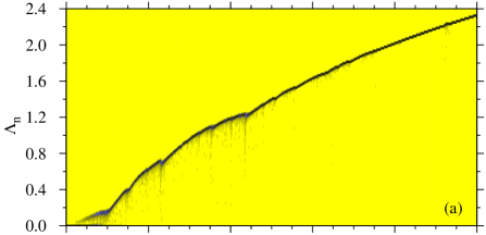
Figure 2a shows the FTLEs distributions $P(\Lambda_{n},K)$ as a function of the nonlinearity parameter $K$ for $400$ initial conditions and up to $n=10^{7}$ iterations. For each initial condition we reckon one FTLE $\Lambda_{n}$, which is the time average of all local FTLE along the trajectory. In Fig. 2a the color changes from light to dark (white over yellow and blue to black) with increasing $P(\Lambda_{n},K)$.

The gray points below the main curve are related to FTLEs from chaotic trajectories which were trapped for a while close to regular islands. For these trapped chaotic trajectories (or “sticky” motion) the local FTLE decreases and consequently the final $\Lambda_{n}$ also decreases. In such cases the FTLE distribution is not Gaussian anymore but contains interesting information about the dynamics. Figure 2a also reveals that for some specific values of $K$ the amount of sticky trajectories changes, which will be quantified and characterized next. Note, that such information is not provided by the mean FTLE shown in Fig. 2b.

2.1 Quantitative characterization of the distributions

Clearly, anomalies in the FTLE distribution reflect sticky motion - however, the entire distribution is not a convenient tool to identify and measure sticky motion. Instead, we will analyze the following four measures:

a.)

The number of occurencies of the most probable FTLEs $P(\Lambda_{n}^{p},K)\equiv{\cal P}_{\Lambda}(K)$ which informs how many initial conditions (normalized) lead to the mode of the distribution [22, 23, 24]. ${\cal P}_{\Lambda}(K)=1$ means that for all initial conditions the FTLEs are equal (within the precision $10^{-3}$). Therefore we expect ${\cal P}_{\Lambda}(K)=1$ for a totally chaotic (or totally regular) system and large times. In cases the sticky motion appears or if the normal distribution did not converge to the given precision, ${\cal P}_{\Lambda}(K)<1$.

b.)

The variance defined by

$$\tilde{\sigma}={\left<(\Lambda_{n}-\left<\Lambda_{n}\right>)^{2}\right>},$$ (5)

which is the second cummulant of the FTLE distribution. It should increase for sticky motion. We will analyze the properties of the relative variance $\sigma=\tilde{\sigma}/\left<\Lambda_{n}\right>^{2}$ which is more appropriate for higher-dimensional systems. In such cases it is possible to detect small differences relative to each unstable direction.

c.)

The skewness is defined by

$$\kappa_{3}=\frac{\left<(\Lambda_{n}-\left<\Lambda_{n}\right>)^{3}\right>}{\tilde{\sigma}^{3/2}}.$$ (6)

It is the third cummulant of the FTLE distribution and detects the asymmetry of the distribution around its mean value. For $\kappa_{3}=0$ we have the regular distribution. Since sticky motion usually reduces the FTLE, the asymmetry of the distribution leads to $\kappa_{3}<0$.

d.)

The kurtosis is defined by

$$\kappa_{4}=\frac{\left<(\Lambda_{n}-\left<\Lambda_{n}\right>)^{4}\right>}{\tilde{\sigma}^{2}}-3,$$ (7)

and detects the shape of the distribution. When $\kappa_{4}>0$ indicates that the distribution is flatter than the regular distribution ($\kappa_{4}=0$), while $\kappa_{4}<0$ reveals a sharper distribution than the normal one.

These four quantities will be used to characterize the degree of sticky motion in the transition from low- to higher-dimensional systems. Altogether they should give all relevant informations which can be extracted from the distributions.

2.2 The two-dimensional case ($d=2$)

To compare with the higher dimensional cases to be discussed later we summarize here $d=2$ results for the FTLEs distributions of the standard map in a slightly different $K$ regime than considered by [6].

Figure 3: (Color online) Deviations from the mean Lyapunov exponent in the interval $K=(7.0,9.0)$ for the standard map measured with (a) ${\cal P}_{\Lambda}(K)$, (b) $\sigma(K)$, (c) $\kappa_{3}(K)$ and (d) $\kappa_{4}(K)$.

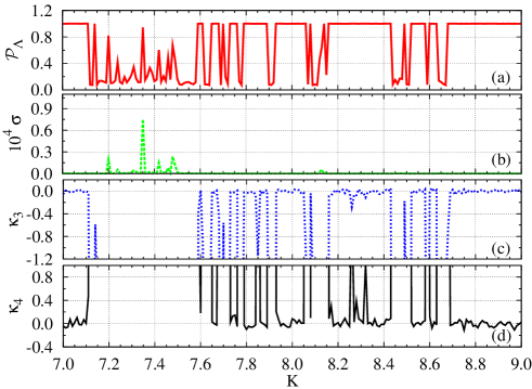
For all simulations we have used $201$ values of $K$ in the interval $K=(7.0,9.0)$ (stepsize $\Delta K=0.01$). As can be seen from Fig. 3a ${\cal P}_{\Lambda}$ has many minima in the interval $K=(7.0,9.0)$. For all minima of ${\cal P}_{\Lambda}$ a certain amount of sticky motion is expected. This is indeed true, as we have checked constructing the PSS (not shown) for some values of $K$ where minima in ${\cal P}_{\Lambda}$ appear and for all of them we found sticky motion. Comparing ${\cal P}_{\Lambda}$ with Fig. 3b we see that $\sigma$ has maxima only for values of $K$ in the interval $(7.15,7.55)$ and close to $8.12$, i.e., the variance does not detect all the sticky regions. However, skewness (Fig. 3c) and kurtosis (Fig. 3d) detect sticky motion as identified by ${\cal P}_{\Lambda}$ in (Fig. 3a). Both parameters behave as expected. In Fig. 3c we plotted the skewness $\kappa_{3}$ as a function of $K$. For almost all minima of ${\cal P}_{\Lambda}$ we observe that the skewness (Fig. 3c) is negative. This implies that the sticky motion induces a left asymmetry in the FTLEs distribution. In other words, the tail on the left side of the distribution is larger than the tail on the right side. For almost all minima of ${\cal P}_{\Lambda}$ the kurtosis $\kappa_{4}$ (Fig. 3d) has a maximum. This is expected since a small ${\cal P}_{\Lambda}$ implies widely distributed $\Lambda_{n}$ and consequently a relatively flat distribution (large $\kappa_{4}$).

Obviously, in the two-dimensional case ${\cal P}_{\Lambda}$, and the cummulants $\kappa_{3}$ and $\kappa_{4}$ are sensitive and consistent detectors of sticky phase space trajectories, with the latter two being more sensitive, while ${\cal P}_{\Lambda}$ is less sensitive, but gives additional information (see, e.g., the interval $K=(7.2,7.5)$), which will become more obvious in the higher dimensional cases.

3 Coupled conservative maps

Coupled conservative maps are convenient systems to investigate sticky motion in higher dimensional phase space systematically. The equations for $N$ coupled conservative maps read

$$S:\left\{\begin{array}[]{l}p_{n+1}^{(k)}=p_{n}^{(k)}+K\,\sin(x_{n}^{(k+1)}-x_{n}^{(k)}),\\ \\ x_{n+1}^{(k)}=x_{n}^{(k)}+p_{n+1}^{(k)},\end{array}\right.$$ (11)

where $k=1,\ldots,N$. We consider periodic boundary conditions $p^{(N+1)}=p^{(1)},~{}x^{(N+1)}=x^{(1)}$ and unidirectional next nearest neighbor coupling. In Eq. (11) we must use modulus $2\pi$. Translational invariance occurs in the $x$–coordinate and the Lyapunov spectrum always possesses two null exponents since two eigenvalues from the Jacobian of the coupled maps are equal to $1$. For $N=2$ our model can be written has a time-one map of a delta-function kicked Hamiltonian flow and the translational symmetry implies, via Noethers theorem, that the total momentum $P_{2}=p_{n}^{(1)}+p_{n}^{(2)}$ is a constant of motion. However, for $N>2$ our model cannot be written as a time-one map of a Hamiltonian flow and the total momentum $P_{N}=\sum_{k}p_{n}^{(k)}$ is not a constant of motion anymore (Noethers theorem is applied for Hamiltonian systems). In all numerical simulations we checked that the sum of all LEs is close to $10^{-14}$ and that their come in pairs.

In addition, the condition $x_{n}^{(k+1)}-x_{n}^{(k)}=n\pi$, for $n=0,1,2\ldots$ is equivalent to the trivial uncoupled maps case $K=0$, where the linear momentum $p_{n}^{(k)}$ of each site is a constant of motion. Very close to this condition we can use the approximation $\sin(x_{n}^{(k+1)}-x_{n}^{(k)})\approx x_{n}^{(k+1)}-x_{n}^{(k)}$, and the total momentum becomes an approximated conserved quantity for any $N$. This will be nicely observed in the simulations when stickiness occurs.

3.1 $N=2\,(d=4)$: The separable case

In this case the system Eq. (11) has one positive, one negative and two zero FTLEs. We show results related to the positive FTLE in Fig. 4.

Figure 4: (Color online) Comparison of (a) $\left<\Lambda_{n}\right>$ (the curve $N=1$ shows results for the standard map calculated at $2K=(14,18)$, see text) with (b) ${\cal P}_{\Lambda}$, (c) $\sigma(K)$, (d) $\kappa_{3}(K)$ and (e) $\kappa_{4}(K)$ in the interval $K=(7.0,9.0)$ and for $N=2$.

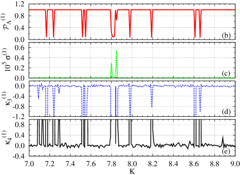
Clearly, the mean value $\left<\Lambda_{n}\right>$ increases with $K$ (Fig. 4a). For $N=2$ the equations of $S$ (11) decouple in center of mass and relative coordinates. The map in the relative coordinate is the standard map but with parameter $2K$. Therefore, the curve in Fig. 4a should match those obtained for the standard map with parameter values $2K=(14,18)$. To check this we plotted $\left<\Lambda_{n}\right>$ in Fig. 4a (dashed line) for the standard map with values $2K=(14,18)$. Both curves are identical. For all minima of ${\cal P}_{\Lambda}$ (Fig. 4b) the skewness $\kappa_{3}$ (Fig. 4d) and the kurtosis $\kappa_{4}$ (Fig. 4e) have also minima and maxima, respectively. At the corresponding values of $K$ many trapped trajectories are expected. Since this case is the standard map with larger nonlinearity parameter ($2K$), we do not discuss further details.

3.2 $N=3\,(d=6)$: The largest FTLE is most sensitive to sticky motion

The case $N=3$ has six FTLEs, two positive, two negative and two zero. The analysis will be done for the distributions of the two positive FTLEs which are labeled such that $\Lambda_{n}^{(1)}>\Lambda_{n}^{(2)}$. For $N=3$ the interval $(7.0,9.0)$ does not exhibit structures in the FTLE distributions pointing to sticky trajectories.

Figure 5: (Color online) Mean values for the two positive FTLEs $\Lambda_{n}^{(1)}>\Lambda_{n}^{(2)}$ for $N=3$.

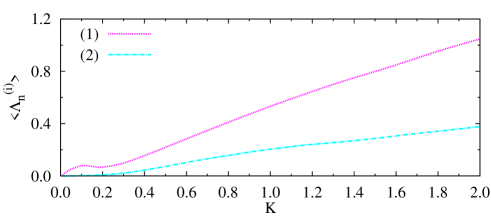
Hence, we analyze the interval $K=(0.01,2.0)$ which is close to the non-chaotic case $K=0$. Figure 5 shows the mean values of the first and second FTLEs as a function of $K$. Both FTLEs increase with $K$, but $\Lambda_{n}^{(1)}$ increases faster and has a minimum close to $K\sim 0.2$. Close to this value $\Lambda_{n}^{(2)}$ starts to be finite. Figures 6 and 7 show the quantities (a) ${\cal P}_{\Lambda}^{(i)}(K)$, (b) $\sigma^{(i)}$, (d) $\kappa_{3}^{(i)}(K)$ and (d) $\kappa_{4}^{(i)}(K)$ as a function of $K$ for $\Lambda_{n}^{(i=1)}$ and $\Lambda_{n}^{(i=2)}$, respectively.

Figure 6: (Color online) Comparison of (a) ${\cal P}_{\Lambda}^{(1)}(K)$ with (b) $\sigma^{(1)}(K)$, (c) $\kappa_{3}^{(1)}(K)$ and (d) $\kappa_{4}^{(1)}(K)$ in the interval $K=(0.01,2.0)$ and $N=3$.

Figure 7: (Color online) Comparison of (a) ${\cal P}_{\Lambda}^{(2)}(K)$ with (b) $\sigma^{(2)}(K)$, (c) $\kappa_{3}^{(2)}(K)$ and (d) $\kappa_{4}^{(2)}(K)$ in the interval $K=(0.01,2.0)$ and $N=3$.

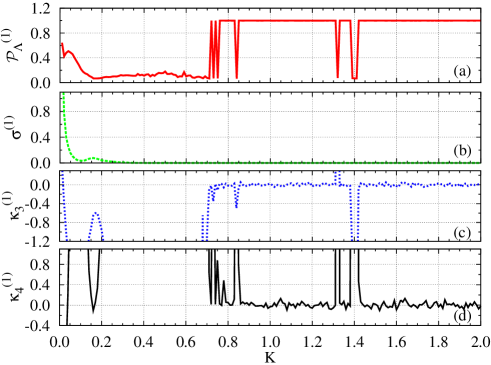
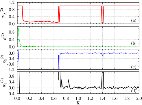
By comparing these plots we see that both distributions detect the sticky motion for $0.1\lesssim K\lesssim 0.7$. In this region the minimum value of $\kappa_{3}^{(i)}(K)$ is $\sim-50$ for $i=1$ and $-30$ for $i=2$. The maximum value of $\kappa_{4}^{(i)}(K)$ is $4000$ for $i=1$ and $\sim 2000$ for $i=2$. For $K\lesssim 0.1$ we observe in Fig. 7 that ${\cal P}_{\Lambda}^{(2)}(K)=1$, meaning that all initial conditions lead to the same $\Lambda^{(2)}_{n}\sim 0.0$. However, $\kappa_{3}^{(2)}(K)$ and $\kappa_{4}^{(2)}(K)$ show that the distribution around $\Lambda^{(2)}_{n}\sim 0.0$ is not Gaussian. By changing $K=0.01\rightarrow 0.1$ the distribution changes slightly from the right asymmetric form [$\kappa_{3}^{(2)}(0.01)\sim 1$] to the left asymmetric form [$\kappa_{3}^{(2)}(0.1)\sim-3$]. The kurtosis is always flat ($\kappa_{4}^{(2)}>-3$) but approaches a regular distribution when $K\sim 0.05$. Similar behavior is observed in Fig. 6 for $\kappa_{3}^{(1)}(K)$ and $\kappa_{4}^{(1)}(K)$. The relative variance is shown to be relevant only at very low values of $K$ (for both FTLEs).

For $K\gtrsim 0.7$ the distribution related to $\Lambda^{(1)}_{n}$ detects the sticky motion at $K\sim 0.83,1.40$ and $K\sim 1.32$, while for $\Lambda^{(2)}_{n}$ it detects $K\sim 1.40$ and $K\sim 0.83$ (but only $\kappa_{4}^{(2)}(K)$). This shows the intuitively expected result that when the nonlinearity parameter increases the most unstable dimension (related to $\Lambda^{(1)}_{n}$) is more sensitive to the sticky motion.

3.3 $N=5\,(d=10)$: The smallest FTLE defines a critical nonlinearity $K_{d}$

Figure 8: (Color online) Mean values for the four positive FTLEs $\Lambda_{n}^{(1)}>\Lambda_{n}^{(2)}>\Lambda_{n}^{(3)}>\Lambda_{n}^{(4)}$ for $N=5$.

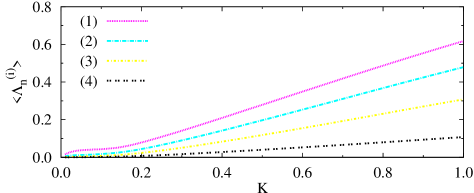
In Fig. 8 the mean values for the positive FTLEs $\Lambda_{n}^{(1)}>\Lambda_{n}^{(2)}>\Lambda_{n}^{(3)}>\Lambda_{n}^{(4)}$ are shown as a function of $K$. For smaller values of $K\lesssim 0.15$, $<\Lambda_{n}^{(3)}>$ and $<\Lambda_{n}^{(4)}>$ are almost zero, while $<\Lambda_{n}^{(1)}>$ increases initially very fast for $K=0.01\rightarrow 0.05$ and then slowly for $K=0.05\rightarrow 0.15$. For $K$ above $0.2$ all mean FTLEs increase linearly with different slopes size-wise ordered as the FTLEs themselves.

Figure 9: (Color online) (a) ${\cal P}_{\Lambda}^{(i)}(K)$, (b) $\sigma^{(i)}(K)$, (c) $\kappa_{3}^{(i)}(K)$ and (d) $\kappa_{4}^{(i)}(K)$ in the interval $K=(0.01,1.0)$, $N=5$ and for all $i=1,2,3,4$.

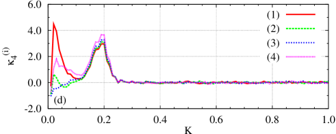
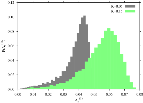
Figure 9 shows that for $K\gtrsim 0.3$ the distributions from all FTLEs approach the normal (Gaussian) form expected for a totally chaotic regime in contrast to the cases $N=1,2,3$ discussed before, where sticky motion also occurs for higher values of $K$. Therefore, there is a clear transition from the quasiregular to the totally chaotic dynamics at $K_{c}\sim 0.3$ simultaneously in all unstable directions. On the other hand, all quantities detect the sticky motion for $K\lesssim 0.25$. Interestingly, above a critical value $K_{d}\sim 0.13$, the four indicators of sticky motion have a similar qualitative behavior for all FTLEs, i. e., independently of the unstable directions. For example, the distributions for all FTLEs have a small left asymmetry ($\kappa_{3}\sim-0.75$) with no flatness ($\kappa_{4}\sim 0$) at $K=0.13$, and a left asymmetry ($\kappa_{3}\sim-1.50$) with flatness ($\kappa_{4}\sim 3.0$) at $K=0.2$. Two exemplary distributions are shown in Fig. 10 for $K=0.05$ and $K=0.15$. Left asymmetry and flatness are evident.

Figure 10: (Color online) Distributions of the FTLEs for $K=0.05$ and $K=0.15$.

The critical value $K_{d}\sim 0.13$ is the point where ${\cal P}_{\Lambda}^{(4)}(K)$ detects the sticky motion from the distribution of the last (the smallest) FTLE [see Fig. 9a]. The value of $K_{d}$ can also be determined approximately from the onset of linear $K$-dependence of the mean FTLEs in Fig. 8.

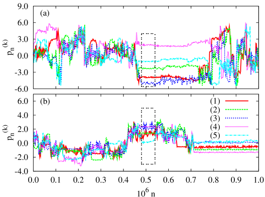
These results show that the sticky motion induces differences between the distributions of $\Lambda_{n}^{(i)}$ only for $K<K_{d}$. Since sticky motion is a consequence of regular structures in phase space, this suggests that there could exist independent invariant regions in phase-space. In the interval $K_{d}<K<K_{c}$ on the other hand, the sticky motion affects all unstable dimensions by the same amount leading to similar distributions for different FTLEs. Finally, in the totally chaotic regime $K>K_{c}$ all unstable directions are affected proportionally to each other. To explain this better we show in Fig. 11 the time evolution of $\Lambda_{n}^{(i)}$ ($i=1,2,3,4$) for one exemplary trajectory in the three distinct regions of $K$. Figure 11(a) shows the behavior of the FTLEs for $K=0.6>K_{c}$ and no sticky motion is observed since no FTLE goes to zero for some shorter time intervals. For the intermediate case $K_{d}<K=0.15<K_{c}$ we see in Fig. 11(b) that for times around $0.5\times 10^{6}$ (see arrow) all four FTLEs are zero, so the sticky motion occurs in all unstable directions and a common behavior is observed. Physically what happens is that the linear momentum of each site becomes approximately constant during sticky motion. This is clearly shown in Fig.12(a), where $p_{n}^{(k)}\ (k=1,2,3,4,5)$ is plotted as a function of $n$. At the sticky time $n\sim 0.5\times 10^{6}$ (see black box), $p_{n}^{(k)}$ is constant for all sites.

Figure 11: (Color online) Time evolution of $\Lambda_{n}^{(i)}$ ($i=1,2,3,4$) for one exemplary trajectory with $N=5$ and (a) $K=0.6>K_{c}$, (b) $K_{d}<K=0.15<K_{c}$, (c) $K=0.05<K_{d}$.

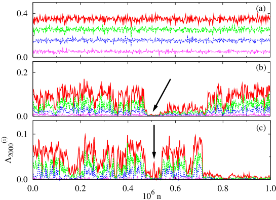
This agrees with the conjecture made by Froeschlé [32] and observed later in coupled maps by [20], i. e., that a conservative system with $N\geq 3$ has $N$ or one (the energy) constants of motion. In other words, following this conjecture when the sticky motion occurs all FTLEs should temporarily be very close to zero, as already observed. However, this changes when the region $K<K_{d}$ is analyzed, as can be observed in Fig. 11(c) for times around $0.5\times 10^{6}$ and $0.85\times 10^{6}$ (see arrows). Only $\Lambda_{n}^{(1)}$ is larger and the remaining three FTLEs are very close to zero. In this case, at the sticky time $n\sim 0.5\times 10^{6}$ (see black box), the momenta $p_{n}^{(1)},p_{n}^{(3)}$ and $p_{n}^{(5)}$ are not conserved anymore. See Fig. 12(b).

Figure 12: (Color online) Time evolution of $p_{n}^{(k)}$ ($k=1,2,3,4,5$) for the trajectory from fig 11 (a) $K_{d}<K=0.15<K_{c}$, (b) $K=0.05<K_{d}$. Black boxes show the sticky region.

3.4 $N=10\,(d=20)$

The case $N=10$ has nine positive FTLEs. In this section we analyze again the interval $K=(0.01,1.0)$ but with $10^{3}$ initial conditions only.

Figure 13: (Color online) Mean values for the nine positive FTLEs $\Lambda_{n}^{(1)}>\Lambda_{n}^{(2)}>\ldots>\Lambda_{n}^{(9)}$, for $N=10$.

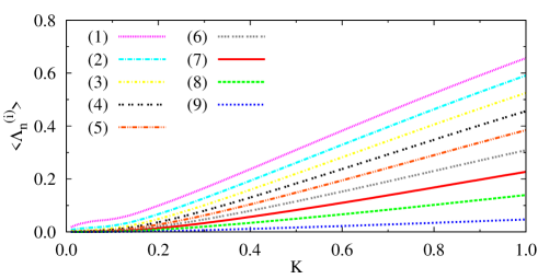
In Fig. 13 the mean values for the FTLEs are plotted as a function of $K$. For $K\gtrsim 0.2$ all mean FTLEs increase linearly and the largest ones increase faster. For $K\lesssim 0.2$ the $K$ dependence is different for different FTLEs. For $K\lesssim 0.1$ almost all (but two $i=1,2$) are very close to zero.

Figure 14: (Color online) Quantities (a) ${\cal P}_{\Lambda}^{(i)}(K)$, (b) $\sigma^{(i)}(K)$, (c) $\kappa_{3}^{(i)}(K)$ and (d) $\kappa_{4}^{(i)}(K)$ as a function of $K=(0.01,1.0)$, for $i=1\rightarrow 9$ and $N=10$.

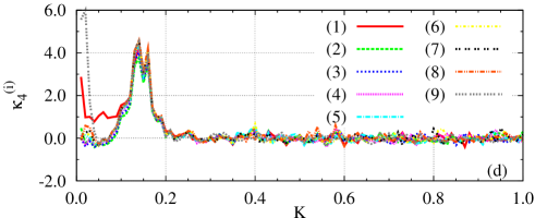
Figure 14 compares (a) ${\cal P}_{\Lambda}^{(i)}(K)$, (b) $\sigma^{(i)}(K)$, (c) $\kappa_{3}^{(i)}(K)$ and (d) $\kappa_{4}^{(i)}(K)$ in the interval $K=(0.01,1.0)$ for all positive FTLEs ($i=1\rightarrow 9$). For $K>K_{c}\sim 0.28$ all quantities indicate that the distributions from all FTLEs approach the normal form expected for a totally chaotic regime. Therefore, again we have a clear transition from quasi-regular to totally chaotic dynamics at $K_{c}$ which occurs simultaneously in all unstable directions. For $K<K_{c}$ all quantities detect the sticky motion. Also here we observe that for $K$ above the critical value $K_{d}\sim 0.09$ the four quantities behave similarly, independent of the FTLEs. The distributions for all FTLEs have a small left asymmetry ($\kappa_{3}\sim-0.75$) with no flatness ($\kappa_{4}\sim 0$) at $K=0.13$, and a left asymmetry ($\kappa_{3}\sim-1.50$) with flatness ($\kappa_{4}\sim 3.0$) at $K=0.2$. The critical value $K_{d}\sim 0.09$ is again exactly the point where ${\cal P}_{\Lambda}^{(9)}(K)$ detects the sticky motion from the distribution of the last (the smallest) FTLE [see Fig. 9(a)]. It can be observed that the distribution of the largest FTLE is the last (when $K$ increases from $0.01$) to “join” the common behavior for $K_{d}\gtrsim 0.09$ [please see Fig. 14(b)-(d)]. The value $K_{d}$ can also be determined approximately from the region in Fig. 13 where the $K$ dependence of the mean FTLEs is not linear.

Figure 15 shows the time evolution of $\Lambda_{n}^{(i)}$ ($i=1\rightarrow 9$) for one exemplary trajectory in the three distinct regions of $K$. In Fig. 15(a) with $K=0.6>K_{c}$ no sticky motion is observed since no FTLE goes to zero for some shorter time intervals. For the intermediate case $K_{d}<K=0.15<K_{c}$ we see in Fig. 15(b) the two different scenarios as conjectured. For times around $0.22\times 10^{6}$ (see arrow) all nine FTLEs are close to zero indicating that the sticky motion occurs in all unstable directions. For times around $0.8\times 10^{6}$ (see arrow) on the other hand, eight FTLEs go to zero but the largest one remains positive.

Figure 15: (Color online) Time evolution of $\Lambda_{n}^{(i)}$ ($i=1\rightarrow 9$) for one exemplary trajectory with $N=10$ and (a) $K=0.6>K_{c}$, (b) $K_{d}<K=0.15<K_{c}$, (c) $K=0.05<K_{d}$.

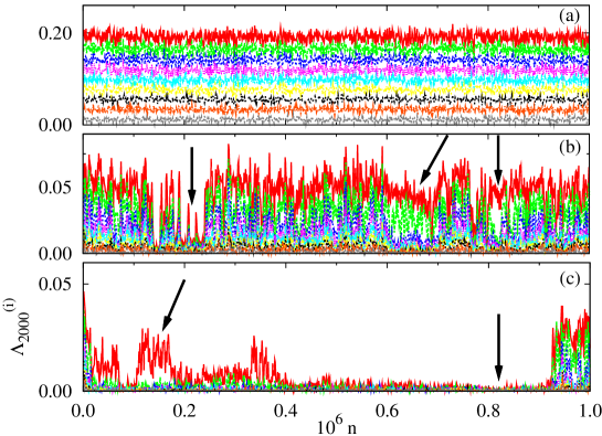
This behavior is observed even more clearly in the region $K<K_{d}$, see Fig. 15(c). For times in the interval $0.12\times 10^{6}$ to $0.18\times 10^{6}$ only $\Lambda_{n}^{(1)}$ is large and the remaining eight FTLEs are very close to zero.

4 Conclusions

It is well known that the dynamics of conservative systems consists of qualitatively different types of motion, from regular over quasi-regular to chaotic, depending on the perturbation parameter. It is difficult to identify these types of motion in high-dimensional systems, especially in the quasi-regular regime where the sticky motion can suppress Arnold diffusion and distinct stochastic regions with different properties may appear [33, 34]. Therefore, it is very desirable to develop tools which quantify the degree of sticky motion, hyperbolicity and ergodicity. Following ideas from [6] the purpose of the present work is to quantify the degree of sticky motion in the phase space of higher-dimensional systems. To fulfill this task we have systematically analyzed small changes in the FTLE distributions using the skewness $\kappa_{3}$, which detects the asymmetry of the distribution, the kurtosis $\kappa_{4}$, which measures the flatness of the distribution and the normalized number of occurencies of the most probable finite time Lyapunov exponent ${\cal P}_{\Lambda}$, which indicates to which extent all trajectories started are under the influence of the same FTLE.

Using coupled conservative maps with nonlinearity parameter $K$ we show that the quantities $\kappa_{3}(K),\kappa_{4}(K)$ and ${\cal P}_{\Lambda}(K)$ are very sensitive to detect the sticky motion and capable to characterize the dynamics when the dimension $d$ of the system increases ($d=2,4,6,10,20$). Simulations were realized up to times $10^{7}$, which are large enough to detect the sticky motion but not too large to destroy the sticky effect on the distribution, which for infinite times should approach the $\delta-$function. This should be valid for not too small values of the nonlinearity $K$. For very small values of $K$ and higher dimensions, the large amount of invariant structures make trajectories stay almost all times at the sticky motion. In such cases it is hard to say what times should be used in general. Besides detecting accurately all cases of sticky motion, we found the following additional interesting results: i) ($d=6$) the largest FTLE is most sensitive to the sticky motion; ii) ($d=10,20$) the smallest FTLE defines the critical nonlinearity parameter $K_{d}$, below which independent invariant regions in phase-space are expected and $\Lambda_{n}^{(i)}(K)$ behaves nonlinearly. For $K>K_{c}$ a clear transition from the quasiregular to the totally chaotic dynamics occurs simultaneously in all unstable directions. In the interval $K_{d}<K<K_{c}$ all quantities detect the presence of sticky motion and distributions for different FTLEs behave similarly, meaning that the sticky motion affects all unstable directions proportionally by the same amount and a kind of common behavior of the distributions is observed. Physically what happens is that the linear momentum of all sites is constant at the sticky motion.

Close-to-zero FTLEs play also an important role in other higher-dimensional system, for example in connection to hydrodynamic modes [35, 36] (among others) and the analysis of hyperbolicity [6, 37]. Results of the present work contribute to categorize the rich and complicated quasiregular dynamics of higher-dimensional conservative systems and also to understand how nonlinearity is distributed along different unstable directions [19, 38].

5 Acknowledgments

The authors thank FINEP (under project CTINFRA-1) for financial support. C.M. also thanks CNPq for financial support and Prof. Giulio Casati for the hospitality by the Center for Nonlinear and Complex Systems at the Università dell’Insubria where part of this work was done.

References

- [1] A. J. Lichtenberg, M. A. Lieberman, Regular and Chaotic Dynamics, Springer-Verlag, 1992.
- [2] G. M. Zaslavsky, Hamiltonian chaos and fractional dynamics, University Press, Oxford, 2008.
- [3] G. Lapeyre, Chaos, 12 (2002) 688.
- [4] F. Ginelli, P. Poggi, A. Turchi, H. Chaté, R. Livi, A. Politi, Phys. Rev. Lett. 99 (2007) 130601.
- [5] E. G. Altmann, H. Kantz, Europhys. Lett. 78 (2007) 10008.
- [6] S. Tomsovic, A. Lakshminarayan, Phys. Rev. E 76 (2007) 036207.
- [7] C. Froeschlé, CH. Froeschlé, Celestial Mechanics and Dynamical Astronomy 56 (1993) 307.
- [8] V. I. Oseledec, Trans. Moscow Math. 19 (1968) 197.
- [9] P. Grassberger, R. Badii, A. Politi, J. Stat. Phys. 51 (1988) 135.
- [10] E. J. Kostelich, I. Kan, C. Grebogi, E. Ott, J. A. Yorke, Physica D 109 (1997) 81.
- [11] M. Falcioni, U. Marini Bettolo Marconi, A. Vulpiani, Phys. Rev. A 44 (1991) 2263.
- [12] M. A. Sepúlvedad, R. Badii, E. Pollak, Phys. Rev. Lett. 63 (1989) 1226.
- [13] M. Ding, T. Bountis, E. Ott, Phys. Lett. A 151 (1990) 395.
- [14] C. Amitrano, R. S. Berry, Phys. Rev. Lett. 68 (1992) 729.
- [15] C. Amitrano, R. S. Berry, Phys. Rev. E 47 (1993) 3158.
- [16] D. Begie, A. Leonard, S. Wiggins, Phys. Rev. Lett. 70 (1993) 275.
- [17] J. D. Szezech, S. R. Lopes, R. L. Viana, Phys. Lett. A 335 (2005) 394.
- [18] M. Harle, U. Feudel, Chaos, Solitons & Fractals 31 (2007) 130.
- [19] P. Grassberger, H. Kantz, Phys. Lett. A 113 (1985) 167.
- [20] H. Kantz, P. Grassberger, Phys. Lett. A 123 (1987) 437.
- [21] R. Artuso, C. Manchein, Phys. Rev. E 80 (2009) 036210.
- [22] M. W. Beims, C. Manchein, J. M. Rost, Phys. Rev. E 76 (2007) 056203.
- [23] H. A. Oliveira, C. Manchein, M. W. Beims, Phys. Rev. E 78 (2008) 046208.
- [24] C. Manchein, M. W. Beims, Chaos Solitons & Fractals 39 (2009) 2041.
- [25] X. Wang, M. Zahn, C. Lai, Y. Lai, Phys. Rev. Lett. 92 (2004) 074102.
- [26] S. S. Negi A. Prasad, R. Ramaswamy, Int. J. Bifurcation Chaos Appl. Sci. Eng. 11 (2001) 291.
- [27] U. Feudel, J. Kurths, A. S. Pikovsky, Physica D 88 (1995) 173.
- [28] C. Grebogi, E. Ott, S. Pelikan, J. A. Yorke, Physica D 13 (1984) 261.
- [29] B. V. Chrikov, Phys. Rep. 52 (1979) 263.
- [30] G. Benettin, L. Galgani, A. Giorgilli, J.-M. Strelcyn, Meccanica 15 (1980) 09.
- [31] A. Wolf, J. B. Swift, H. L. Swinney, J. A. Vastano, Physica D 16 (1985) 285.
- [32] C. Froeschlé, Phys. Lett. A 16 (1972) 172.
- [33] M. Pettine, A. Vulpiani, Phys. Lett. 106A (1984) 207.
- [34] R. Livi, A. Politi, S. Ruffo, A. Vulpiani, J Stat. Phys. 46 (1987) 147.
- [35] H. L. Yang, G. Radons, Phys. Rev. Lett. 100 (2008) 024101.
- [36] M. Romero-Bastida, E. Braun, J. Phys. A 41 (2008) 375101.
- [37] J. C. Vallejo, R. L. Viana, M. A. F. Sanjuan, Phys. Rev. E 78 (2008) 066204.
- [38] C. Manchein, J. Rosa, M. W. Beims, Physica D 238 (2009) 1688.