Experimental estimation of entanglement at the quantum limit

Abstract

Entanglement is the central resource of quantum information processing and the precise characterization of entangled states is a crucial issue for the development of quantum technologies. This leads to the necessity of a precise, experimental feasible measure of entanglement. Nevertheless, such measurements are limited both from experimental uncertainties and intrinsic quantum bounds. Here we present an experiment where the amount of entanglement of a family of two-qubit mixed photon states is estimated with the ultimate precision allowed by quantum mechanics.

Entanglement is the central resource of quantum information processing and the precise characterization of entangled states is a crucial issue for the development of quantum technologies. In turn, quantification and detection of entanglement have been extensively investigated, see ren1 ; ren2 ; ren3 for a review, and different approaches have been developed to extract the amount of entanglement of a state from a given set of measurement results bayE ; Wun09 ; Eis07 ; KA06 . Of course, in order to evaluate the entanglement of a quantum state one may resort to full quantum state tomography LNP which, however, becomes impractical in higher dimensions and may be affected by large uncertainty TE94 . Other methods, requiring a reduced number of observables, are based on visibility measurements Jae93 , Bell’ tests b1 ; c2 ; w3 , entanglement witnesses h1 ; t2 ; G3 or are related to Schmidt number pas ; fed . Many of them found an experimental application mg ; wei ; ser ; nos , also in the presence of decoherence effects buc06 ; dav07 .

Any quantitative measure of entanglement corresponds to a nonlinear function of the density operator and thus cannot be associated to a quantum observable. As a consequence, ultimate bounds to the precision of entanglement measurements cannot be inferred from uncertainty relations. Any procedure aimed to evaluate the amount of entanglement of a quantum state is ultimately a parameter estimation problem, where the value of entanglement is indirectly inferred from the measurement of one or more proper observables EE08 . An optimization problem thus naturally arises, which may be properly addressed in the framework of quantum estimation theory qet1 ; qet2 , which provides analytical tools to find the optimal measurement and to derive ultimate bounds to the precision of entanglement estimation.

Suppose one has a family of quantum states $\varrho_{\epsilon}$ labeled by the value of entanglement, say negativity, and wants to estimate $\epsilon$ from the outcomes $\chi=(x_{1},..,x_{N})$ of $N$ repeated measurements of the (generalized) observable described by a Positive Operator Valued Measurement (POVM) $\Pi_{x}$, $\sum_{x}\Pi_{x}=\openone$. Any inference strategy amounts to find an estimator, i.e. a map $\hat{\epsilon}(\chi)$ from the experimental sample to the parameter space. According to the Cramer-Rao theorem the precision of any estimation procedure, i.e. the variance of any unbiased estimator based on the measurement of $\Pi_{x}$ is bounded by the inequality $\hbox{Var}(\hat{\epsilon})\geq[NF_{\epsilon}]^{-1}$, where $F_{\epsilon}=\sum_{x}p(x|\epsilon)\,[\partial_{\epsilon}\ln p(x|\epsilon)]^{2}$ is the Fisher information and $p(x|\epsilon)=\hbox{Tr}[\varrho_{\epsilon}\>\Pi_{x}]$ is the conditional probability of getting the outcome $x$ when the actual value of entanglement is $\epsilon$. Upon maximizing the Fisher information over all the possible quantum measurements we arrive at the quantum Fisher information (QFI) $F_{\epsilon}\leq H_{\epsilon}=\hbox{Tr}[L_{\epsilon}^{2}\rho_{\epsilon}]$ expressed in terms of the symmetric logarithmic derivative $L_{\epsilon}$, i.e. the selfadjoint operator satisfying the equation $\partial_{\epsilon}\rho_{\epsilon}=\frac{1}{2}(L_{\epsilon}\rho_{\epsilon}+\rho_{\epsilon}L_{\epsilon})$. The ultimate bounds to precision are thus determined by the quantum Cramer-Rao bound (QCRB) $\hbox{Var}(\hat{\epsilon})\geq[NF_{\epsilon}]^{-1}\geq[NH_{\epsilon}]^{-1}$. The meaning of QCRB is that quantum mechanics does not allow entanglement estimation with arbitrary precision. In turn, QCRB represents the ultimate bound to the precision of any procedure aimed to estimate the amount of entanglement of a state belonging to the family $\varrho_{\epsilon}$. In order to optimally estimate entanglement we thus need i) a measurement with Fisher information $F_{\epsilon}=H_{\epsilon}$ equal to the QFI and ii) an estimator saturating the Cramer-Rao bound LQE . In EE08 , bounds to precision have been evaluated for several classes of pure and mixed quantum states. Here we demonstrate experimentally for the first time that optimized correlations measurements allows for the estimation of entanglement with the ultimate precision imposed by quantum mechanics. In particular, we present the results of an experiment to estimate the amount of entanglement (negativity) of two-qubit photon states. This represents a substantial advance, paving the way for further progresses. In fact, with a judicious choice of correlation measurements one can devise a procedure to optimally estimate entanglement for a generic class of two-photon entangled states.

The family of entangled states we are dealing with is made of polarization entangled photon pairs obtained by coherently superimposed type-I parametric downconversion (PDC) generated in two BBO crystals mg . The experimental set-up is schematically depicted in Fig. 1. A CW Argon pump laser beam with wavelength $\lambda=351nm$ is filtered with a dispersion prism and then passes through a Glan-Thompson prism with horizontal axis of transmission that selects the polarization $|H\rangle$. An halfwave plate WP0 rotates the polarization by the angle $\phi$, which in turn determines the amount of entanglement in the output state. PDC light is generated by two thin type-I BBO crystals (l=1mm), positioned with the planes that contain optical axes orthogonal to each other. PDC occurs only in crystal 1(2) if the polarization of the pump beam is horizontal(vertical).

Figure 1: (Color online) Experimental setup to generate polarization entangled photon pairs with variable entanglement and estimate its value with the ultimate precision allowed by quantum mechanics.

The crystals are cut for collinear frequency degenerate phase-matching at working wavelength and the phase shifts due to ordinary and extraordinary path in the crystals are compensated by rotating the quartz plates QP. To maintain stable phase-matching conditions, BBO crystals and QP are placed in a closed box which is kept heated at fixed temperature. Overall, the output states are described by the family of density matrices $\varrho_{\epsilon}=p|\psi_{\phi}\rangle\langle\psi_{\phi}|+(1-p)D_{\phi}$ which represent the mixing of the ideal pure entangled states $|\psi_{\phi}\rangle=\cos\phi|HH\rangle+\sin\phi|VV\rangle$ (negativity $\epsilon=\sin 2\phi$) with a small fraction of a separable mixture $D_{\phi}=\cos^{2}\phi|HH\rangle\langle HH|+\sin^{2}\phi|VV\rangle\langle VV|$. The angle $\phi$ may be tuned at will upon rotating the waveplate WP0, whereas the mixing parameter $p$ comes from the decoherence mechanisms occurring in the experimental setup. These are mostly due to fluctuations of the relative phase between the two polarization components, which themselves derive from residual temperature fluctuations: in order to obtain different mixed states these fluctuation are eventually magnified by eliminating the isolating box. The entanglement (negativity) of the state $\varrho_{\epsilon}$ is given by $\epsilon=p\sin{2\phi}$ and its purity by $\mu=1-(1-p^{2})\sin{2\phi}$. Upon inverting these relations and express the family of states in terms of $\epsilon$ and $\mu$ or $p$ we may evaluate the QFI for entanglement estimation, which turns out to be a function of $\epsilon$ only, $H_{\epsilon}=(1-\epsilon^{2})^{-1}$. In the following, we describe our detection strategy and show it allows entanglement estimation with precision saturating the QCRB independently on the purity.

After the crystal, the pump is stopped by a filter (UVF), and the biphoton field is split on a non-polarizing 50-50 beam splitter (BS). The measurement stage consists in projecting the beams on vertical polarizers after passing through halfwave plates (WP1, WP2). After spectral selection by an interference filters (IF) centered at the degeneracy 702nm (FWHM=3nm), biphotons are collimated by a short focal length lens and detected on SPAD (D1, D2). Electrical signals from detectors are registered with a coincidence scheme (CC) with a time window of coincidences set to $1ns$. Overall, the measurement scheme is described by projection measurements onto two-qubit states

$$\Pi_{t}(\alpha,\beta)=|\alpha+s\frac{\pi}{2}\rangle\langle\alpha+s\frac{\pi}{2}|\otimes|\beta+s^{\prime}\frac{\pi}{2}\rangle\langle\beta+s^{\prime}\frac{\pi}{2}|$$

where $t=\{s+2s^{\prime}\}$, $s,s^{\prime}=0,1$. The polarization angles $\alpha,\beta$ are set by Glen-Thompson polarizers, whereas the rotations of $\pm\pi/2$ are obtained by putting the half-wave plates WP1 and WP2 at $\pm 22,5^{o}$ (mounted on precision rotation stages with high resolution and fully motor controlled).

Let us first illustrate precision analysis assuming the generation of the pure states $|\psi_{\phi}\rangle$. In this case negativity is given by $\epsilon=\sin 2\phi$ and the estimation of entanglement reduces to a measurement of coincidence rates in a two-particle interferometer setting Jae93 . Indeed, upon inspecting the expression of the probabilities $p_{t}(\epsilon;\alpha,\beta)=\langle\psi_{\phi}|\Pi_{t}(\alpha,\beta)|\psi_{\phi}\rangle$, $t=0,1,2,3$ one finds out that an unbiased estimator for the negativity can be written as $\hat{\epsilon}=V(\alpha,\beta)\csc{2\alpha}\csc{2\beta}-\cot(2\alpha)\cot(2\beta)$, where $V(\alpha,\beta)=p_{0}-p_{1}-p_{2}+p_{3}$ is the expected value of two-qubit quantum correlations (QC). The corresponding Fisher information is thus given by $F_{\epsilon}=\sum_{t}p_{t}(\epsilon;\alpha,\beta)[\partial_{\epsilon}\log p_{t}(\epsilon;\alpha,\beta)]^{2}$ and it equals the QFI, $H_{\epsilon}$, for $\alpha=\pm\pi/4$, $\beta=\pm\pi/4$. In other words $\hat{\epsilon}=V(\pm\pi/4,\pm\pi/4)$, which can be measured with the experimental setup described above, are good candidates for being optimal estimators of entanglement. In practice, at fixed $\phi$, $\alpha$ and $\beta$ and for each measurement run $j=1,..,M$ one records the vector $\mathbf{k}_{j}=\{k_{0,j},k_{1,j},k_{2,j},k_{3,j}\}$, where $k_{t,j}\equiv k_{t,j}(\alpha,\beta)$, is the number of coincidence counts, as measured for the given set of parameters by the coincidence circuit during a single time window ($10$ seconds). For large values of the total number of coincidences $K_{j}=\sum_{t}k_{t,j}$ (determined irrespectively of the polarizers’ orientation in the $j-th$ run), the expected value of the coincidence rate $k_{t,j}(\alpha,\beta)/K_{j}$ converges to the probability $p_{t}(\epsilon;\alpha,\beta)$ and the estimator can thus be written in terms of the coincidences’ vector $\hat{\epsilon}\equiv\hat{\epsilon}(\bf{k}_{j})$. In our implementation we have performed $M=30$ measurements of the coincidence vector for fixed values $\alpha=-\pi/4$ and $\beta=\pi/4$.

For finite $K_{j}$s the uncertainty in the estimation of entanglement are mostly due to fluctuations $\delta k_{t}$ in the coincidence counts $k_{t,j}$ around their average values $\left\langle k_{t}\right\rangle=\sum_{j}k_{t,j}/M$. Using standard error propagation with the derivatives $\partial_{t}\equiv\partial/\partial k_{t}$ evaluated for $k_{t}\equiv\left\langle k_{t}\right\rangle$, and assuming independence among fluctuations at different angles, we have $\hbox{Var}(\hat{\epsilon})=\sum_{t}|\partial_{t}\hat{\epsilon}|^{2}\delta k_{t}^{2}=4[(\left\langle k_{0}\right\rangle+\left\langle k_{3}\right\rangle)^{2}(\delta k_{1}^{2}+\delta k_{2}^{2})+(\left\langle k_{1}\right\rangle+\left\langle k_{2}\right\rangle)^{2}(\delta k_{0}^{2}+\delta k_{3}^{2})]/\left\langle K\right\rangle^{4}$. If we now assume that the counting processes have a Poissonian statistics, i.e. $\delta k_{t}^{2}=\left\langle k_{t}\right\rangle^{2}$, then it is straightforward to prove that

$$\hbox{Var}(\hat{\epsilon})=4(k_{0}+k_{3})(k_{1}+k_{2})/\left\langle K\right\rangle^{3}=(1-\hat{\epsilon}^{2})/\left\langle K\right\rangle$$

i.e. QC measurements allow for optimal estimation of entanglement with precision at the quantum limit. Since the QFI is given by $H_{\epsilon}=(1-\epsilon^{2})^{-1}$ for a wide range of two-qubit families of states EE08 , the above calculations suggest that this is a general result. In other words, given a source emitting polarization two-qubit states with coincidence counting statistics satisfying the Poissonian hypothesis, then the experimental setup of Fig 1 allows for optimal estimation of entanglement at the quantum limit by means of a QC estimator.

This is indeed the case for the experimental setup of Fig. 1 and the family of output states $\varrho_{\epsilon}$ where, upon evaluating the probabilities $p_{t}(\epsilon;\alpha,\beta)=\hbox{Tr}[\varrho_{\epsilon}\>\Pi_{t}(\alpha,\beta)]$, one sees that $\hat{\epsilon}=V(-\pi/4,\pi/4)$ is still an optimal (unbiased) estimator of entanglement. In practice, we have collected $M=30$ repeated acquisitions of coincidence vector $\boldsymbol{k}_{j}=\{k_{0j},k_{1j},k_{2j},k_{3j}\}$, then we have randomized the composition of $\boldsymbol{k}_{j}$ over the sequence of measurements to avoid spurious correlations, and finally we have estimated entanglement as the sample mean $\langle\hat{\epsilon}\rangle=\sum_{j}\hat{\epsilon}(\boldsymbol{k}_{j})/M$. The corresponding uncertainty has been evaluated by the sample variance $\hbox{Var}(\hat{\epsilon})=\sum_{j}[\hat{\epsilon}(\boldsymbol{k}_{j})-\langle\hat{\epsilon}\rangle]^{2}/(M-1)$. In order to compare the estimated value of entanglement with the actual one we need to estimate also the additional parameter $p$, quantifying the amount of mixing introduced by decoherence processes. An unbiased estimator $\hat{p}$ for this parameter may be obtained by measuring QC with a different set of angles, e.g. upon collecting the coincidences $\bf{r}_{j}\equiv\bf{k}_{j}(\alpha=\beta=0)$ to form $\hat{p}(\boldsymbol{r}_{j},\boldsymbol{k}_{j})=\frac{1}{2}\hat{\epsilon}(\boldsymbol{k}_{j})R_{j}/\sqrt{r_{3,j}(1-r_{3,j})}$, where $R_{j}=\sum_{t}r_{t,j}$ is the total number of coincidences with the four orientations $\alpha,\beta=0,\pi/2$. The actual (”true”) value of negativity is then inferred as $\epsilon_{t}=\langle\hat{p}\rangle\>\sin{2\phi}$, i.e. using the knowledge of the rotation angle of the waveplate WP0 and the estimation of the mixing parameter.

Figure 2: Estimation of entanglement at the quantum limit. The plot shows the estimated value of entanglement $\langle\hat{\epsilon}\rangle$ as a function of the actual one $\epsilon_{t}$. The uncertainty bars on $\langle\hat{\epsilon}\rangle$ denotes the quantity $\sqrt{\hbox{Var}(\hat{\epsilon})\times\langle K\rangle}$, i.e. the square root of the sample variance multiplied by the average number of total coincidences $\langle K\rangle$. The gray area corresponds to values within the inverse of the Fisher information $\epsilon_{t}\pm H_{\epsilon_{t}}^{-1/2}$. Uncertainty bars on the abscissae correspond to fluctuations $\delta\epsilon_{t}=\sqrt{\hbox{Var}(\hat{p})}\sin 2\phi$ in the determination of $\epsilon_{t}$, due to fluctuations in the estimation of the mixing parameter.

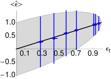
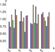
In Fig. 2 we show the estimated value of entanglement as a function of the actual one for seven values of $\phi=10^{\circ},15^{\circ},20^{\circ},28^{\circ},40^{\circ},45^{\circ},45^{\circ}$ of the WP0 rotation angle (corresponding to estimated mixing $\langle\hat{p}\rangle=0.85,0.88,0.88,0.85,0.92,0.93,0.97$ respectively). The uncertainty bars on $\langle\hat{\epsilon}\rangle$ denotes the quantity $\sqrt{\hbox{Var}(\hat{\epsilon})\times\langle K\rangle}$, i.e. the square root of the sample variance multiplied by the average number of total coincidences $\langle K\rangle$. This is in order to allow a direct comparison with the Cramer-Rao bound in term of the inverse of the Fisher information (the gray area). Uncertainty bars on the abscissae correspond to fluctuations $\delta\epsilon_{t}=\sqrt{\hbox{Var}(\hat{p})}\sin 2\phi$ in the determination of $\epsilon_{t}$, due to fluctuations in the estimation of the mixing parameter. As it is apparent from the plot entanglement is estimated with precision at the quantum limit for any value of the the rotation angle $\phi$. Notice that this conclusion is robust against the fact that the statistics is not exactly Poissonian: in the left panel of Fig. 3 we show the Fano factor for the four recorded coincidence counts $k_{j}$ and the six values of $\phi$ employed in the experiment.

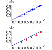
Our statistical model $\varrho_{\epsilon}$ may be checked for consistency on the basis of the recorded data themselves, and other possible models to describe decoherence of our family of states are ruled out as they cannot fit the experimental sample. As for example, if one tries to describe the output from our source by the family of (depolarized) Werner states $\varrho_{\epsilon}^{\prime}=p|\psi_{\phi}\rangle\langle\psi_{\phi}|+\frac{1}{4}(1-p)\openone\otimes\openone$, than one sees from the expression of the coincidence probability $p_{t}^{\prime}(\epsilon;\alpha,\beta)=\hbox{Tr}[\varrho_{\epsilon}^{\prime}\>\Pi_{t}(\alpha,\beta)]$ that unbiased estimators for the mixing parameters and the negativity may be expressed as $\hat{p}^{\prime}=V(0,0)$, $\hat{\epsilon}^{\prime}=-\frac{1}{2}+\frac{1}{2}V(0,0)+V(-\pi/4,\pi/4)$. These may be written in terms of the coincidence vectors $\mathbf{k}$ and $\mathbf{r}$ as $\hat{p}^{\prime}(\boldsymbol{r}_{j})=(r_{r0,j}-r_{1,j}-r_{2,j}+r_{3,j})/R_{j}$ and $\hat{\epsilon}^{\prime}(\boldsymbol{r}_{j},\boldsymbol{k}_{j})=-\frac{1}{2}+\frac{1}{2}\hat{p}^{\prime}(\boldsymbol{r}_{j})+(k_{0,j}-k_{1,j}-k_{2,j}+k_{3,j})/K_{j}$. Upon evaluating the corresponding sample means and variances one realizes that the model is incompatible with the observed data. This is illustrated in the right panel of Fig.3 where we report the estimated value of entanglement as a function of the actual one assuming, for the description of the output signals, the families $\varrho_{\epsilon}$ (top plot) and $\varrho_{\epsilon}^{\prime}$ (bottom plot). Here the uncertainty bars denote the $3\sigma$ confidence interval and thus it is apparent that $\varrho_{\epsilon}^{\prime}$ cannot fit the data. We also performed measurements of the coincidence counts for a complete set of polarization angles and check the model $\varrho_{\epsilon}$ by full two-qubit state tomography KB00 ; Ja01 .

Figure 3: (Color online) Left: Fano factors of the coincidence counts $k_{j}$, $j=0,1,2,3$. Each groups contains the Fano factor for the seven values of $\phi$ reported in the text. Right: estimated value of entanglement as a function of the actual one assuming, for the description of the output signals, the families $\varrho_{\epsilon}$ (top plot) and $\varrho_{\epsilon}^{\prime}$ (bottom plot). The uncertainty bars stays for to the $3\sigma$ confidence interval.

In conclusion, we have suggested and demonstrated a measurement scheme based on quantum correlation measurements to optimally estimate entanglement for a family of two-photon entangled states. Our procedure is self-consistent and allows to estimate the amount of entanglement with the ultimate precision imposed by quantum mechanics. With an appropriate choice of correlation measurements our results may be extended to a generic class of two-photon entangled states. The statistical reliability of our method suggests a wider use in precise monitoring of external parameters assisted by entanglement.

This work has been supported in part by MIUR (PRIN 2007FYETBY), Regione Piemonte (E14), ”San Paolo foundation”, and NATO (CBP.NR.NRCL.983251). MGAP and PG thanks Marco Genoni for several useful discussions.

References

- (1) R. Horodecki et al. Rev. Mod. Phys. 81, 865 (2009).
- (2) O. Gühne, G. Toth, Phys. Rep. 474, 1 (2009).
- (3) R. Augusiak, M. Lewenstein, ArXiv:0906.5264
- (4) P. Lougovski, S. J. Van Enk, ArXiv:0806.4165
- (5) H. Wunderlich, M. B. Plenio, ArXiv:0902.2093
- (6) J. Eisert. F. G. S. L. Brandao, K. M. Adenauert, New J. Phys. 9, 46 (2007).
- (7) K. M. R. Audenaert, M. B. Plenio New J. Phys. 8, 266 (2006).
- (8) Quantum state estimation. Lect. Not. Phys. 649, M. G. A. Paris and J. Rehacek Eds. (Springer, Berlin, 2004).
- (9) G. M. D’Ariano, C. Macchiavello, M. G. A. Paris, Phys. Lett. A 195, 31 (1994).
- (10) G. Jaeger, M. A. Horne, A. Shimony, Phys. Rev. A 48, 1023 (1993).
- (11) J. S. Bell, Speakable and Unspeakable in Quantum Mechamics, (Cambridge University Press, Cambridge, 2004).
- (12) J. F. Clauser, M. A. Horne, A. Shimony, and R. A. Holt, Phys. Rev. Lett. 23, 880 (1969).
- (13) R. F. Werner and M. Wolf, Quant. Inf. Comp. 1, 1 (2001).
- (14) M. Horodecki, P. Horodecki, and R. Horodecki, Phys. Lett. A 223, 1 (1996).
- (15) B. M. Terhal, Phys. Lett. A 271, 319 (2000).
- (16) O. Guhne, P. Hyllus, D. Bruss, A. Ekert, M. Lewenstein, C. Macchiavello, and A. Sanpera, Phys. Rev. A 66, 062305 (2002).
- (17) P. Facchi, G. Florio, S. Pascazio, Int. Journ. of Q. Inf. 5 (2007) 97.
- (18) M.V. Fedorov, M.A. Efremov, P.A. Volkov, and J.H. Eberly, J. Phys. B 9, S467 (2006).
- (19) M. Genovese, Phys. Rep. 413, 319 (2005).
- (20) M.Bourennane et al., Phys. Rev. Lett. 92, 087902 (2004).
- (21) M.V. Fedorov et al., Phys. Rev. Lett, 99, 063901 (2007); Phys. Rev. A, 77, 032336 (2008).
- (22) G.Brida et al., arXiv:0904.3009.
- (23) S.P. Walborn et al. Nature 440, 1022 (2006); A.R. Ribeiro de Carvalho et al. Phys. Rev. Lett. 98, 190501 (2007).
- (24) M. P. Almeida et al. Science, 316 , 579 (2007).
- (25) M. G. Genoni, P. Giorda, M. G. A. Paris Phys. Rev. A 78, 032303 (2008).
- (26) C. W. Helstrom, Phys. Lett. A 25, 1012 (1967); C. W. Helstrom, Quantum Detection and Estimation Theory (Academic Press, New York, 1976); A.S. Holevo, Statistical Structure of Quantum Theory, Lect. Not. Phys 61, (Springer, Berlin, 2001).
- (27) C. W. Helstrom, Phys. Lett. A 25, 1012 (1967); S. Braunstein and C. Caves, Phys. Rev. Lett. 72, 3439 (1994); S. Braunstein, C. Caves, and G. Milburn, Ann. Phys. 247, 135 (1996); D. C. Brody, L. P. Hughston, Proc. Roy. Soc. Lond. A 454, 2445 (1998); A 455, 1683 (1999).
- (28) M. G. A. Paris, Int. J. Q. Inf. 7 125, (2009).
- (29) K. Banaszek, G.M. D’Ariano, M.G.A. Paris, and M.F. Sacchi, Phys. Rev. A 61 10304 (2000).
- (30) D.F.V. James, P.G. Kwiat, W.J. Munro, and A.G. White, Phys. Rev. A 64, 052312 (2001);
- (31) Y. Bogdanov et al., Phys. Rev. A 70, 042303 (2004).