FCNC and CP Violation Observables in a –flavoured MSSM
Abstract
A non-Abelian flavour symmetry in a minimal supersymmetric standard model can explain the flavour structures in the Yukawa couplings and simultaneously solve the SUSY flavour problem. Similarly the SUSY CP problem can be solved if CP is spontaneously broken in the flavour sector. In this work, we present an explicit example of these statements with a flavour symmetry and spontaneous CP violation. In addition, we show that it is still possible to find some significant deviation from the SM expectations as far as FCNC and CP violation are concerned. We find that large contributions can be expected in lepton flavour violating decays, as and , electric dipole moments, and and kaon CP violating processes as . We also show that without further modifications, it is unlikely for these models to solve the anomaly at low-moderate . Thus, these flavoured MSSM realizations are phenomenologically sensitive to the experimental searches in the realm of flavor and CP violation physics.
I Introduction
In the next few years, after a long impasse in the phenomenological searches for new physics in the energy frontier, all the high-energy particle physics community will be focused on the results from the LHC experiments. Its first goal will be the study of the physics of electroweak symmetry breaking, but besides this, we also expect some kind of new physics around the electroweak scale. Supersymmetry (SUSY) is perhaps the new physics option that is best motivated. The LHC should find some SUSY particles if SUSY is indeed the solution to the hierarchy problem and provides a candidate for the dark matter observed in the universe.
Supersymmetry has been extensively studied in the last decades, but most of these studies have been done in the framework of the so-called Constrained Minimal Supersymmetric Standard Model (CMSSM). The CMSSM is one of the simplest supersymmetric extensions of the Standard Model as it assumes universality of the supersymmetric soft breaking terms and is completely determined by four parameters () plus a sign (sg()). This simplified model is very useful to explore the main features of the SUSY spectrum in collider experiments, however, nobody really believes that the realization nature has chosen of supersymmetry is exactly the CMSSM, specially concerning flavour. In analogy to the known flavour structures in the Yukawa couplings, we naturally expect non-trivial flavour structures in the supersymmetry soft-breaking terms.
Therefore, we should consider other more general flavoured MSSM models as the SUSY models we can find when we analyze the experimental results from LHC experiments. Nevertheless, it is well-known that the presence of generic flavour structures in the SUSY soft-breaking terms causes the so-called “supersymmetric flavour problem”. Flavour changing neutral currents (FCNC) and flavour-dependent CP violation observables receive too large contributions from loops involving SUSY particles and can not satisfy the stringent phenomenological bounds on these processes Masiero:2001ep ; Masiero:2005ua . Although this statement is still true, it is important to emphasize that the basis of this problem lies clearly on our total ignorance about the origin of the observed flavour and CP-violation in our theory, and this includes also the SM Yukawa couplings. The real flavour problem is simply our inability to understand the complicated structures in the quark and lepton Yukawa couplings, and likewise for the soft-breaking flavour structures in the MSSM. It has been recently shown in the literature Ross:2004qn ; Calibbi:2008qt that an MSSM model with a non-Abelian flavour symmetry allows a simultaneous understanding of the flavour structures in the Yukawa couplings and the SUSY soft-breaking terms, adequately suppressing FCNC and CP violating phenomena and solving the SUSY flavour problem.
In this work, we intend to exhibit a concrete example of such strategy considering an MSSM (with the limited number of new parameters present in the CMSSM) and showing that the presence of a non-Abelian family (horizontal) symmetry can simultaneously account for the solution of both flavor problems, namely that it is possible to successfully reproduce the correct fermion spectrum while adequately suppressing FCNC and CP violating phenomena. Regarding the phenomenology of these flavoured MSSM models, we do not expect large differences from the expectations in the CMSSM from the point of view of collider studies, as we know that the departures from flavour universality are strongly constrained by the present FCNC and CP violation experiments. Much probably the resolution of the new supersymmetric flavour structures will have to rely on FCNC and CP violation experiments. In the following we will analyze the FCNC and CP violation phenomenology of our flavoured MSSM example. We will show that it is still possible to find some significant deviation from the the SM expectations as far as the FCNC and CP violations are concerned, making these realizations phenomenologically sensitive to the experimental searches in the realm of flavor physics.
In the next section, we introduce the flavour symmetries in SUSY and study its effects in the SUSY soft-breaking terms. Then, we illustrate these effects with an explicit model with a flavour symmetry. In section III, we analyze the different FCNC and CP violation observables in this model including lepton flavour violation, kaon physics, physics and electric dipole moments. Section IV is devoted to a combined analysis of all the FCNC and CP violation observables and we show the correlations between the most interesting observables in this model. Finally, in section V we present our conclusions.
II Flavour Symmetries in SUSY
Flavour symmetries have been used with success in the past to try to extract some meaning from the complicated structures of fermion masses and mixings in the Standard Model (SM). Using the Froggat-Nielsen mechanism Froggatt:1978nt , flavour symmetries explain the structure of the SM Yukawa couplings as the result of a spontaneously broken symmetry associated with flavour. In different extensions of the SM, these flavour symmetries will also constrain the new couplings and masses. For instance, in the context of a supersymmetric theory, a flavour symmetry would apply equally to the fermion and scalar sectors. Therefore, this implies that in the limit of exact symmetry the soft-breaking scalar masses and the trilinear couplings must be invariant under the flavour symmetry and the structures in the soft-breaking terms will be generated after the spontaneous breaking of the flavour symmetry. Both the flavour structures in the Yukawa couplings and in the soft-breaking terms are generated by the same mechanism and thus we can expect a close relation between them111The relation between the soft-breaking terms and the Yukawa matrices is present in gravity mediation mechanisms, but it would not be present if the mediation mechanism is flavour blind, as in the case of gauge mediation or anomaly mediation.
The flavour-diagonal scalar masses, i.e. couplings , are clearly invariant under any symmetry and are always allowed by the flavour symmetry. However, in general, this does not guarantee that they are family universal. In the case of an Abelian Froggatt:1978nt ; Leurer:1992wg ; Pomarol:1995xc ; Binetruy:1996xk ; Dudas:1996fe ; Dreiner:2003yr ; Kane:2005va ; Chankowski:2005qp family symmetry, the symmetry does not relate different generations, and, generically, different fields will have different diagonal soft masses. On the other hand, a non-Abelian family symmetry groups two or three generations in a single multiplet with a common mass in the symmetric limit, thus helping to solve, in principle, the FCNC problem. This was one of the main motivations for the construction of the first flavour models Barbieri:1995uv ; Barbieri:1996ww , where the first two generation sfermions, facing the strongest constraints, share a common mass. In the case of an flavour symmetry King:2001uz ; King:2003rf ; Ross:2004qn ; deMedeirosVarzielas:2005ax , all three generations have the same mass in the unbroken family symmetry limit. On the contrary, trilinear couplings are completely equivalent to the Yukawa couplings from the point of view of the symmetry because they involve exactly the same fields (scalar or fermionic components). Thus, they are generated after symmetry-breaking as a function of small vevs. Therefore, to solve the “SUSY flavour problem”, we will consider in this work non-Abelian family symmetries, and more exactly theories or discrete versions of this symmetry.
Apart from these renormalizable mass operators in the Lagrangian, we can construct non-renormalizable operators neutral under the flavour symmetry inserting an appropriate number of flavon fields. The flavon fields, charged under the symmetry, are responsible for the spontaneous symmetry breaking once they acquire a vev. Then, higher dimensional operators involving two SM fermions and a Higgs field, with several flavon vevs suppressed by a large mediator mass, generate the observed Yukawa couplings. In the same way, these flavon fields will couple to the scalar fields in all possible ways allowed by the symmetry and, after spontaneous symmetry breaking, they will generate a non-trivial flavour structure in the soft-breaking parameters. Therefore, by being generated by insertions of the same flavon vevs, we can expect the structures in the soft-breaking matrices and the Yukawa couplings to be related.
The structure in the Yukawa couplings is not completely determined by the observed values of fermionic masses and mixing angles. To solve this problem and fix the Yukawa couplings, we accept that the smallness of CKM mixing angles is due to the smallness of the off-diagonal elements in the Yukawa matrices with respect to the corresponding diagonal elements, and we make the additional simplifying assumption of choosing the matrices to be symmetric. With these two theoretical assumptions, and using the ratio of masses at the GUT scale to define the expansion parameters in the up and down sector as and , we can fix the Yukawa textures in the quark sector to be:
| (7) |
where , and the are coefficients fixed by the observed values of fermion masses and mixings. In the Appendix we show the full structure of the Yukawas, and find the best fit values , , , , , . In the leptonic sector we will follow the same strategy as in Ref. Calibbi:2008qt and require unification of charged lepton and down-quark flavour matrices, i.e. we embed our model in a grand unified framework, for instance , and we try to explain simultaneously quark and lepton Yukawas. The detailed structure of the leptonic Yukawa matrix is also shown in the Appendix.
Taking this Yukawa structure as our starting point, we will generate the flavour structure of the soft-breaking terms in generic non-Abelian flavour symmetries or discrete versions, like or deMedeirosVarzielas:2005qg ; deMedeirosVarzielas:2006fc ; Kobayashi:2006wq ; Ishimori:2008uc ; Ishimori:2009ew . Under these symmetries, the three generations of SM fields, both -doublets and singlets, are triplets and the Higgs fields are singlets. Therefore Yukawa couplings and trilinear terms are not allowed by the symmetry. In these models, we add several flavon fields. For instance in Ross:2004qn we have , (anti-triplets ), and (triplets ), while in deMedeirosVarzielas:2005ax we have also and . The symmetry is broken in several steps, first is broken into by the vev of and , with and being of the same order as the mediator mass , i.e. . Subsequently and get a smaller vev , with and . Notice that in principle, we have three different mediator masses, , because the flavour symmetry must commute with the SM symmetry and therefore the vector-like mediator fields must have the SM quantum numbers of the usual particles222For simplicity, we take and in all our numerical calculations.. In some models we also have and getting a lower vev with .
Notice that the mentioned vevs require a vacuum alignment mechanism. In this work we do not specify a particular mechanism, but we refer the interested reader to the examples in Ross:2004qn ; Altarelli:2005yp ; deMedeirosVarzielas:2005qg ; Kobayashi:2008ih ; Seidl:2008yf .
The basic structure of the Yukawa superpotential (for quarks and leptons) is then given by
| (8) |
in the absence of fields, or,
| (9) |
in the models with . All flavon fields in these equations should be understood as . Note, however, that the symmetry is not enough by itself to determine the required structure in the superpotential. Generically, we have to introduce additional global symmetries to forbid unwanted terms, like a mixed term , that would spoil the Yukawa structure. Nevertheless, the structure in Eqs. (8) and (9) is quite general for the different models we can build, and for additional details we refer to King:2001uz ; King:2003rf ; Ross:2004qn .
In the same way, the scalar soft masses deviate from exact universality after breaking. As explained above, is completely neutral under gauge and global symmetries and gives rise to a common contribution for the family triplet. However, after breaking, terms with additional flavon fields give rise to important corrections Ross:2002mr ; Ross:2004qn ; Antusch:2007re ; Olive:2008vv . Any invariant combination of flavon fields can also contribute to the sfermion masses (at least with Planck scale suppression). In this case, it is easy to see that the following terms will always contribute to the sfermion mass matrices (the presence of the field will depend on the model):
| (10) |
where represents the quark and lepton doublets or the up (neutrino) and down (charged-lepton) singlets, so that . From here we see that taking , both models with and without have the same structure up to corrections that will be always subdominant in the relevant soft mass matrices in the basis of diagonal Yukawa matrices.
Notice that in Eq. (II) only the fields that enter the superpotential have their vevs and associated mediators masses fixed by the or parameters. For instance in the discrete model of Ref.deMedeirosVarzielas:2006fc , (the -field that in this reference is written as ) does not enter the superpotential. Therefore, its contributions to the soft masses can be suppressed even having a large vev if the associated mediator mass is high enough333We thank G. G. Ross and I. de Medeiros Varzielas for clarifying this point.. However, in the continuous version of this model deMedeirosVarzielas:2005ax , the vevs of and are constrained to be both by D-flatness and thus they are not dangerous in the soft-mass matrices. Moreover, we have to remember that these deviations from universality in the soft-mass matrices proportional to flavour symmetry breaking come always through corrections in the Kähler potential and these effects will be important only in gravity-mediation SUSY models.
In the case of the trilinear couplings we have to emphasize that from the point of view of the flavour symmetry these couplings are completely equivalent to the corresponding Yukawa coupling. This means that they necessarily involve the same combination of flavon vevs, although order one coefficients are generically different because they require at least an additional coupling to a field mediating SUSY breaking (in general coupled in different ways in the various contributions). Therefore, from our point of view, we expect that the trilinear couplings have the same structure as the Yukawa matrices in the flavour basis. However in general they are not proportional to the Yukawas, because of different coefficients in the different elements. Thus, we can expect that going to the SCKM basis does not diagonalize the trilinear matrices. In fact, the trilinear matrices maintain the same structure as in the flavour basis and only the coefficients are modified.
Therefore, we can see that in these -like models with the three generations unified in a single field, we have basically the same “leading order” structures in the soft mass matrices and the trilinear couplings directly related to the structures in the Yukawa couplings. In the following we concentrate in the model of Ross:2004qn because it has a complete phase structure in the flavon vevs consistent with the CKM phase. Remember however, that the main features of the soft terms are similar in other models and in principle the phase structure could be also adapted in these models.
II.1 SU(3) Flavour Model
Let us now specify more explicitely the flavour model that we use as our main example. The full superpotential is determined by and several global symmetries are used to forbid unwanted terms that would spoil the observed structure of the Yukawa couplings. Using the charges presented in Table 2, the leading terms in the superpotential are,
| (11) | |||||
where to simplify the notation, the flavon fields have been normalized to the corresponding mediator mass, which means that all the flavon fields in this equation should be understood as . The field is a Georgi-Jarlskog field that gets a vev in the direction, distinguishing leptons and quarks. Furthermore, as said above this model is embeded in a grand unified structure at high scales, which allow us to relate quark and lepton (including neutrino) Yukawa couplings. However, the subgroup of must be broken as we need different mediator masses for the up and down sector and, in fact and are representations of which is broken by their vevs Ross:2002fb ; King:2003rf ; Ross:2004qn .
After spontaneous symmetry breaking the flavon fields get the following vevs:
| (22) | ||||||
| (29) |
where we require the following relations:
| (30) |
These relations are valid at the flavour breaking scale, that we take as the GUT scale in the numerical evaluation.
| Flavon Phase | ||||
|---|---|---|---|---|
| Allowed Values | Unconstrained |
It is straight-forward to see that this superpotential reproduces correctly the required Yukawa structure in Eq. (7). For completeness, we also list in Table 1 the values that the flavon phases can take, given the constraints imposed by the CKM matrix. The analysis leading to such constraints is found in the Appendix.
We can now turn to the soft breaking terms. As mentioned in the previous section, a universal, flavour diagonal mass term will always be allowed. Moreover, in a SUSY theory, the same messenger fields as in the Yukawas will couple the flavons to the scalar fields in the soft terms. Thus, the and parameters still act as expansion parameters, and represent important corrections to the soft terms.
Clearly any coupling involving a flavon field and its hermitian conjugate (i.e. ) is invariant under the flavour symmetry. From this we can deduce that the soft mass terms get a minimum structure determined uniquely by the flavon content of the model and on their vevs. This minimum structure is obtained from the following effective terms:
| (31) |
In Table 2 we show a choice of global charges that reproduces the correct Yukawa structure and does not allow other terms at leading order in the Kähler potential (soft-masses).
| 3 | 3 | 1 | 1 | 3 | 3 | |||
| 0 | 0 | 0 | 1 | 0 | -1 | 1 | 0 | |
| -1 | -1 | 0 | 2 | 1 | 0 | -1 | 4 | |
| 1 | 1 | 0 | -3 | -1 | 1 | 0 | -4 |
In the squark sector, after rephasing the fields such that the CKM matrix elements , , and are real, the soft masses in the SCKM basis are:
| (32d) | |||||
| (32h) | |||||
| (32l) | |||||
| (32p) | |||||
| (32t) | |||||
where () is in the basis where () is diagonal, is related to the CKM phase, and . The and phases can be found in the Appendix. The structure of in the basis where is diagonal is similar to . Notice that, although the structure in terms of , in and is the same as that of and , respectively, the coefficients from the SCKM rotation and RGE evolution are different due to the Georgi-Jarlskog field . This can be seen in the Appendix, and is summarized in Table 5, in Section III.1. The phase structure of the slepton matrices is different to the one of squarks, since the latter have been rephased in order for the CKM matrix to follow the standard phase convention.444As physical observables are independent of phase conventions, we could also rephase the slepton superfields and use the same phase structure as squarks.
In Eq. (32), we have written only the leading contribution in and to each element with a leading phase, omitting effective complex coefficients. This sets the size of the modulus of the mass-insertion. The coefficients are the remaining part of the full element, after factorizing the terms explicitly written in Eq. (32). There are many contributions to these coefficients: first, we have the real constants in front of each term in the Kähler potential, at . We also have contributions from the real constants in the Yukawa matrices, coming from the rotation into the SCKM basis. A third contribution comes from the RGE evolution to the EW scale. And finally, it is possible to have further contributions from subleading terms in the Kähler potential, still at .
All of these contributions can involve the flavon phases, so the effective can be complex. As we are factorizing the leading phases, the phase in each coefficient shall only appear in subleading terms. If the leading phases cancel for a particular observable, these subleading phases shall be important. Such a cancellation can happen in EDMs. For example, in mass-insertion notation Gabbiani:1996hi ; Hagelin:1992tc , the corresponding effective coefficients of and have the following structure:
| (33a) | |||||
| (33b) | |||||
Although Eq. (II.1) is the minimal structure present for all possible models, it is possible, for particular choices of the global symmetries and charges, to build other symmetry-dependent soft-mass structures. In fact, the observed structure in the Yukawa couplings does not fix completely the introduced global charges and it is possible to add new invariant combinations of flavon fields to the Kähler potential without modifying the Yukawas.
| 3 | 3 | 1 | 1 | 3 | 3 | |||
| -2 | -2 | 0 | -4 | 2 | 3 | 0 | -2 | |
| 0 | 0 | 0 | 1 | 0 | -1 | 1 | 0 |
The first example of these new combinations of flavon fields in the Kähler is achieved by allowing a term (RVV2). The required charges are shown in Table 3. It is easy to check that, with these charges, the structure of the Yukawa couplings in the superpotential remains unchanged. This is due to the fact that the superpotential is a holomorphic function of the fields while the Kähler is only a real function. When rotated to the SCKM basis, the soft-mass matrices become:
| (34d) | |||||
| (34h) | |||||
| (34l) | |||||
| (34p) | |||||
| (34t) | |||||
One can see that the effect of this term in is to exchange one power of by a suppression in and . In , the same terms change an by an . However, for , and considering that , such replacements leave the structure of the mass matrices very similar numerically to the original one (notice that and are taken at ). Nonetheless, it must be remarked that the phase structure of the whole mass matrix is modified.
As in RVV1, it is crucial to take into account that relative phases exist within the effective coefficients. For instance, although the global phase of is still , the structure of in RVV2 is now:
| (35) |
Notice that the factor does not really provide any suppression at all. This means that the imaginary part of is larger than just . We label this new, larger, effective phase as .
| 3 | 3 | 1 | 1 | 3 | 3 | |||
| -1 | -1 | 0 | 5 | 1 | -2 | 0 | 6 | |
| 0 | 0 | 0 | -1 | 0 | 0 | 1 | -2 |
A second possibility is to allow a term (RVV3) in the Kähler, with the charges being shown in Table 4. The soft matrices, when rotated into the SCKM basis, have the following structure:
| (36d) | |||||
| (36h) | |||||
| (36l) | |||||
| (36q) | |||||
| (36u) | |||||
with defined in the Appendix.
This model shows larger deviations from RVV1 in the sector. It is important to notice that is now of order instead of , which will have considerable consequences in processes such as . Likewise, is of order instead of , so an enhancement in should be expected. Regarding the sector, for , the suppression at has roughly the same size as an suppression, so once again the structure of is numerically similar to RVV1 for this value of .
The trilinear couplings, on the other hand, follow the same symmetries as the Yukawas. Thus, they have the same flavon structure in RVV1, RVV2 and RVV3. Nonetheless, although they have the same structure, they do not have the same constants, which means that the rotation into the SCKM basis does not diagonalize them. In the SCKM basis, after rephasing the fields, the trilinears have the following structure:
| (37d) | |||
| (37h) | |||
where we have neglected the coefficients. One can get by taking with .
The soft mass matrices in Eqs. (32,34,36,37) are given at the large scale . Then, we have to include also effects coming from the running from to . Although these effects produce further non-universal contributions, they are usually smaller than the terms presented here. In the quark sector, the misalignment of the and matrices gives sizeable contributions to the and sectors, analogous to the MFV contributions of CMSSM models. In the lepton sector with RH neutrinos, the same happens due to the misalignment of and Borzumati:1986qx ; Casas:2001sr ; Masiero:2002jn . Both of these contributions are unavoidable, albeit the contribution is highly model dependent.
Moreover, in the present case there are new contributions to the running given by the intrinsic non-universality of the soft mass matrices. Although these effects contribute even in the sector, it turns out that the magnitude of the generated off-diagonal terms are, at most, of the same order as those at . This means that the addition of running effects will only change the already unknown constants, such that the low-energy phenomenology can still be understood by analyzing Eqs. (32), (34), (36) and (37).
Finally, we have to emphasize once more that all the soft matrices presented here have unknown coefficients in all non-universal terms. The flavour symmetry allows us to fix the order in and of the different entries but the final values could easily vary up or down by factors of two and this has to be taken into account when analyzing our numerical results.
III FCNC and CP Violation Observables
In the following, we shall study flavour and CP violating observables, presenting analytical estimates in mass insertion approximation (MIA). Moreover, we will perform a full numerical analysis in the SUGRA parameter space through a scan in and for fixed values of and . The numerical analysis is done defining the Yukawa, trilinear and soft mass matrices at GeV, for the three different versions of the model, as explained in Section II.1. Then the different flavour matrices are evolved to the electro-weak scale, solving 1-loop RGEs with SPheno Porod:2003um . coefficients in the Yukawa matrices are determined by requiring a good fit on the fermion masses and quark mixings at Roberts:2001zy . The result of such fit is presented in the Appendix.
Regarding the unknown constants in both the superpotential and Kähler potential, as we do not have a full high-scale model, we shall fix each s at a random value, between and 2. Notice they can be of either sign. Thus, a model is characterized by both the choice of symmetries involved, and by the particular s we have in front of each effective term. In Section IV we shall take into account their variation.
After running the resulting matrices down to the scale, we diagonalize the Yukawas in order to obtain the left and right mixing matrices and rotate the soft matrices into the SCKM basis. At the scale, for each point of the SUSY parameter space, we compute the SUSY spectrum and check that the electroweak symmetry breaking does take place and no tachyonic particles arise. Moreover, to be conservative, we require that the Lightest Supersymmetric Particle (LSP) is the lightest neutralino.
In this work we do not include the non-holomorphic corrections to the Yukawa couplings, so our results are valid for low and moderate values of . In this regime, the effects of these non-holomorphic corrections are usually small. The only exception is found in the case for the neutron EDM, where new imaginary parts induced by these corrections can give sizeable contributions. We give details on how we introduce such corrections to this observable in Section III.4.
Finally, we apply the following constraints:
-
•
Bounds on the sparticle masses from direct searches at LEP and Tevatron Amsler:2008zzb .
-
•
Lower bound on Higgs masses from LEP Barate:2003sz . Although the SM bound on the Higgs mass is of 114 GeV, in SUSY the modification of the lightest Higgs coupling could reduce this constraint. In order to take this effect into account, for each point we calculate the Higgs mixing angle and use Eq. (17) of Ref. Djouadi:2001yk to estimate the correct Higgs mass bound. We then use SPheno to calculate the two loop Higgs mass, and take into account a theoretical uncertainty of 3 GeV Allanach:2004rh ; Heinemeyer:2004xw .
-
•
. The experimental world average from the CLEO Chen:2001fja , Belle bellebsg1 and BaBar Aubert:2005cua collaborations is given by hfag-web :
(38) We have to compare these values with the MSSM predictions. In our numerical calculation, we use the expression presented in Ref. Hurth:2003dk in which the branching ratio is explicitly given in terms of arbitrary complex Wilson coefficients and . At present, the SM contribution to this decay is already available at NNLO while the SUSY contribution in a general MSSM is partially known at NLO. In this work, we include the NLO SM contribution with a modified low value of the scale for the charm mass to reproduce the NNLO SM contribution () Degrassi:2007kj ; Becher:2006pu ; Lunghi:2006hc . We add the supersymmetric contributions at one loop, and require that the total result does not deviate from the experimental value of Eq. (38) in more than 2-sigma.
-
•
Muon anomalos magnetic moment, . At present, the experimental result for this observable is given by Bennett:2006fi ,
(39) while, computing the hadronic contribution by means of the hadronic annihilation data, the SM theoretical expectation is Miller:2007kk ; Passera:2008jk ; Jegerlehner:2009ry ,
(40) The resulting discrepancy is:
(41) It is well-known that in the MSSM receives contributions from – and – loops Moroi:1995yh . Such contributions are approximately given by the following expression:
(42) A comparison with Eq. (41) implies that the present discrepancy strongly favours the region of the SUSY parameter space. In the case of the theoretical prediction based on decay Davier:2002dy , the difference of Eq. (41) is reduced to Passera:2008jk but it still requires a positive correction and disfavours strongly a sizable negative contribution.
III.1 Lepton Flavour Violation
As pointed out in Calibbi:2008qt , flavour models based on SU(3) give rise to potentially large rates of LFV processes, such that positive signals of LFV can be found in the currently running or near-future experiments, at least for SUSY masses within the reach of the LHC. The arising of large mixing among flavours relies on the features of the SU(3) model discussed in the previous sections: the presence of nonuniversal scalar masses already at the scale where the SUSY breaking terms appear, and the fact that the trilinear matrices are in general not aligned with the corresponding Yukawa matrices. Let’s start considering the case , where the latter effect is strongly reduced so that, in terms of mass insertions, BR() mainly depends on and . Looking at the structure of the slepton soft mass matrices in the three versions of the model (Table 5), we see that RVV1 and RVV2 are expected to give similar predictions for and , with possibly sizeable contributions coming from both the LL and the RR sector. In the case of RVV3, the prediction for will be also similar to the previous two cases, while we expect to be strongly enhanced. In fact, for RVV3, the LL mass insertion is larger by a factor with respect to RVV1 and RVV2, and the is consequently increased by two orders of magnitude.
| RVV1 | ||||||
|---|---|---|---|---|---|---|
| RVV2 | ||||||
| RVV3 |
| Present Bound | Future Sensitivity | |
|---|---|---|
| Ahmed:2001eh | meg | |
| Banerjee:2007rj ; Lusiani:2007cb | Bona:2007qt | |
| Aubert:2005wa | Akeroyd:2004mj |
To summarize, let’s compare the expections for the different LFV processes. In the case , considering for simplicity only the contribution from , we have:
| (43) | |||||
| (44) |
where () is the () full width. Given the present limits and future sensitivities of LFV processes shown in Tab. 6, we see that is not able to constrain the parameter space better than in none of the three models. On the other hand, we expect from Eq. (44) that the present constraints given by and , that differ by three orders of magnitude, are comparable for RVV1 and RVV2, while should give the strongest constraint in the case of RVV3.
In the case , generally large insertions arise as a consequence of the misalignment between and the corresponding Yukawa matrix . In this case, the neutralino contribution to gets strongly enhanced Calibbi:2008qt and the present (or future) bound requires heavier SUSY masses to be fulfilled, specially in the region where the gaugino mass is much larger than the common sfermion mass. Nevertheless, we expect this effect to be visible only in the case of RVV1 and RVV2, while for RVV3 the very large should still give the dominant contribution.
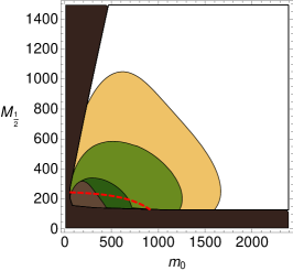
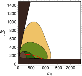
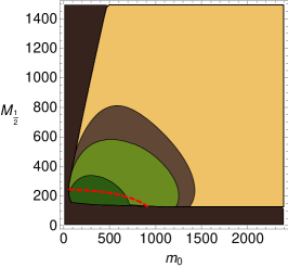
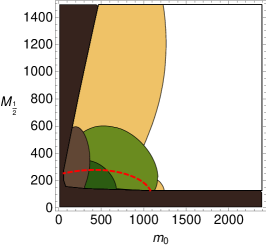
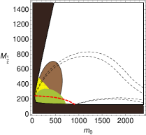
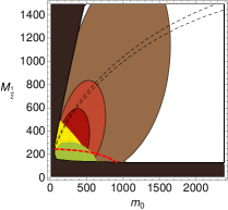
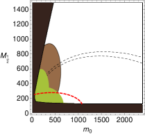
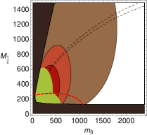
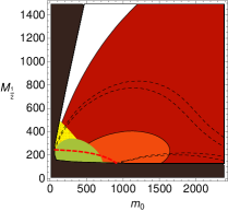
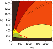
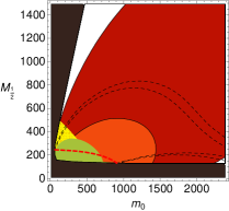
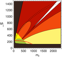
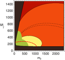
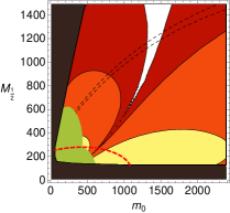
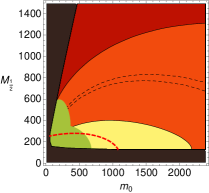
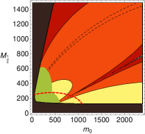
Let us now consider the results of the numerical analysis for the LFV decays. After fixing the unknown parameters to random values, we present in Fig. 1 the current bounds provided by and in the (, ) plane, and also the final reach of the MEG experiment. In the first row, the case is displayed (for ). We see that, as expected, RVV1 and RVV2 give similar results both for and . The regions of the parameter space excluded by the present bounds , are comparable, as obtained by the naive estimate in Eq. (44), although turns out to be more constraining for . The presently allowed region is approximately . In the case of RVV3, already gives a strong constraint, , which is much more stringent than the one provided by . Although the precise values may vary with different parameters, these plots give an idea of the reach of these LFV experiments. As a consequence, for SUSY masses lying within the LHC reach, RVV3 results already rather disfavoured, while RVV1 and RVV2 are not strongly constrained. Considering the sensitivity expected at the MEG experiment for , , we see that also RVV1 and RVV2 will be tested in most of the parameter space accessible to the LHC, while RVV3 will be completely probed well beyond the LHC reach. Moreover, in case of larger values of (e.g. ), since , MEG will be able to test all the displayed parameter space also for RVV1 and RVV2 (cfr. Calibbi:2008qt , where a similar model has been studied).
In the second row of Fig. 1, the three versions of the model are displayed for the case , in order to show the potentially large flavour mixing induced by the A-terms. As expected, we see that, for RVV1 and RVV2, the bound is increased with respect to the case, specially for , as a consequence of the large insertion contributing in diagrams with pure exchange. Also in this case, MEG has a very high capability of testing the parameter space. Indeed, for moderate slepton masses the neutralino contribution is so large that the models will be fully probed. Only in the case of rather heavy sleptons, the can be suppressed enough to escape the reach of MEG. In the case of RVV3, the contribution from LL insertion remains dominant and no substantial changes are observed with respect to the case of vanishing trilinear terms.
As RVV3 is heavily constrained by LFV, in the following we shall exclude it from our analysis, and concentrate exclusively on RVV1 and RVV2.
III.2 Kaon physics
Supersymmetric contributions to – mixing are mainly determined by the mixing between the first two generations of down type squarks. In terms of mass insertions, a major hadronic constraint on comes from . The kaon mass difference, , does constrain . However, this observable is less sensitive to small MIs since the long-distance effects are difficult to estimate.
On the experimental side, current data Amsler:2008zzb shows that and the phase of is . On the theoretical side, many improvements are being made in the determination of input parameters needed to calculate the SM prediction of . We have good information on the CKM matrix elements thanks to the vast amount of data from physics. Also available are new lattice estimates of the parameter which enters the hadronic matrix element. However, these developments have lead to a puzzle in understanding the data. The authors of Refs. Buras:2008nn ; Buras:2009pj realized that within the SM, the theoretical prediction of might not be enough to account for the measured value if one accepts the unitarity triangle (UT) fit using physics observables. One can summarize their result in the numerical form Buras:2008nn ; Buras:2009pj ,
| (45) | ||||
The definition of each symbol and its value can be found in the above references. Notice that the , appearing in this equation refer to the UT angle , not to the ratio of the Higgs vevs in SUSY. The denominator of each fraction is the central value of the input parameter appearing in the numerator, quoted in Ref. Buras:2009pj . Major uncertainties are those in , , , which are 5%, 11%, 7%, respectively. One important refinement made in this expression, which had been overlooked in most of the literature, is the factor that parameterizes suppression of the result due to and the imaginary part of the 0-isospin amplitude of . In addition, latest lattice values of are lower than previous determinations. Here we take Antonio:2007pb ; Allton:2008pn (see also Aubin:2009jh ). These two facts cooperate to make insufficient for the central values, obtaining , which is smaller than the observed by 18%. This deficit should be compensated by some new source; since our model has extra sources of CP violation, we are lead to invoke these new sources to resolve the puzzle.
Before we proceed further, a clarification is in order regarding the puzzle. It stems from the tension among different observables used to determine the UT on the plane. The regions preferred by , , and do not precisely overlap with one another (see Ref. Lunghi:2008aa for example). As we said, if one accepts the regions determined by and , then should be modified. Conversely, one may also conceive a scenario where the region is in fact correct whereas one or more of the sector observables have been contaminated by new physics effects. This could be an equally legitimate solution in a general case. However, it is not viable within our framework. The reason is that supersymmetric contributions to the above three observables are (up to uncertainties) correlated and that the region is modified much more than the other two. We shall add more quantitative comments on this in the next subsection.
In order to evaluate the supersymmetric effects on , we should calculate . For this, we follow Ref. Ciuchini:1998ix which presents the Wilson coefficients from the gluino-squark box graphs (which are the largest SUSY contributions in the presence of sizeable squark mass insertions) and the expressions for evolving those Wilson coefficients from the sparticle mass scale down to the hadronic scale. After that, the SUSY contribution to is given by the formula,
| (46) |
And then we can express the supersymmetric contribution to in terms of mass insertions as,
| (47) | ||||
where and functions and can be found in Ref. Ciuchini:1998ix . We have omitted the term proportional to which happens to contribute only .
In the numerical analysis, we set Antonio:2007pb ; Allton:2008pn and use the central values of from Ref. Nakamura:2006eq .
In our flavour models, RVV1 and RVV2, we have and with different phases in the two models, and respectively, as can be seen from Eq. (32) and the paragraph following Eq. (35). Therefore, we can expect that the supersymmetric contribution to can easily be comparable to , in particular from the contribution in the second term in Eq. (47). The additional contribution might well be just what we need to fill the gap between and , which could amount to 18% or more.
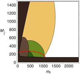
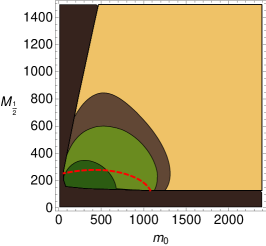
In Figs. 2, we present contours of on the plane for RVV1. The left and the right figures are for positive and negative O(1)’s for , respectively.
The phase of can be either or which are respectively marked in black and gray in Figs. 2. Note that the phase of is and that and should interfere constructively to fit the experimental value. Therefore, gray contours worsen compatibility between the theoretical and the experimental values of by increasing their discrepancy. The phase of is determined by the sign of Eq. (47). It is often dominated by the term proportional to . In this case, the phase of can be shifted by if one multiplies either or by (of course, the modulus does not remain exactly the same due to the first term). For example, we can flip the sign of the RR insertion by changing the signs of the O(1) coefficients in . This is the reason why the region with gray contours on the left plot turns to black on the right.
For RVV2, the phase in is much larger than that in RVV1, as we can see in Eq. (35). This makes the SUSY contribution to dominant in all of the evaluated parameter space, so only one of the two possible phases for solves the tension. Furthermore, each of the contours in Figure 2 would be scaled roughly by a factor .
The requirement that the supersymmetric contribution solves the puzzle would define a strip in this plane which will be shown in all of the following plots, for both RVV1 and RVV2. One virtue of such a strip is that the parameter space therein will lead to a definite correlation between observables which are not apparently related to each other. We will elaborate on this in Sec. IV.
Another important quantity in kaonic CP violation is . It is specially sensitive to chirality-flipping mass insertions, and Gabbiani:1996hi . Using the formulae in Ref. Buras:1999da , one can write the supersymmetric contribution to in the form,
| (48) |
which has been derived for . The constant parameterizes the uncertainty in the hadronic matrix element of the chromomagnetic operator. We have suppressed other factors that can change by for , since the following argument depends only on the order of magnitude of .
In this model, there can be flavor-violating A-terms arising from mismatch of the coefficients between the Yukawas and the A-terms. To estimate their possible effects, we define , with being the overall dimensionful coefficient of the A-terms. Using Eq. (37b) and (32b), one can get rough relationships among different 1–2 mass insertions,
| (49) |
where is the -quark mass at the GUT scale. If we require that the size of the second term in Eq. (47) does not exceed unity, we find that the extra contribution to has an upper limit like
| (50) |
for purely imaginary or . In this case, the supersymmetric fraction within should be lower than 40% for a reasonably high . In fact, the phases of these flavor and chirality changing insertions are which are smaller than maximal, as can be seen from Eq. (74). Thus their effects on are smaller than the above estimate. We have numerically checked that the gluino-squark loop contribution to is less than 15% on the strip compatible with . Given the large theoretical uncertainty in , this amount of contamination by new physics should be hard to disentangle.
Another process that could, in principle, be interesting is the decay Nir:1997tf ; Buras:1997ij ; Colangelo:1998pm . The dominant contribution to this process requires the presence of CP violating phases, and therefore we could expect to have a contribution in our model. As, due to gauge invariance, this decay depends on -breaking, it requires the presence of two Higgs vevs, either within insertions in the squark sector, or within gaugino-higgsino mixing on the neutralino and chargino sectors. At moderate , this disfavours the gluino contribution, since insertions are, at most, proportional to the bottom mass. Of much more interest is the chargino contribution, as the insertions are proportional to the top mass. Nonetheless, the required and insertions depend on powers of , instead of , which constrains greatly any chargino contribution dependent on the structure. The chargino contribution will then be dominated by the flavour-changing of the CKM matrix, and thus cannot present any larger deviations than those predicted by MFV models.
III.3 physics
Let us now discuss new physics effects on mixing. For this, it is convenient to adopt the following parametrization Bona:2008jn :
| (51) |
The – transition amplitude is divided into two parts, one arising from the SM loops and the other from the gluino-squark which are the largest SUSY contributions in our model:
| (52) |
Here, we focus on the phase rather than on , since the hadronic uncertainty in the latter is larger than the extra contributions that can be expected in this model.
The current data of mixing phase is showing an interesting deviation from the SM prediction. A constrained fit, performed by HFAG, results in Barberio:2008fa :
| (53) |
Recall that non-vanishing is an indication of new physics. The above fit is away from the SM at the level of , and the 90% CL range is:
| (54) |
It would be amusing to see whether or not our model could push this phase close to its best fit value.
In order to estimate maximal size of within this model, one should consider the ratio of to appearing in Eq. (51). We follow Ref. Becirevic:2001jj to express the supersymmetric amplitude in terms of mass insertions. The SM amplitude is available in Ref. Buchalla:1995vs for instance. For this, we use and from the full fit by the UTfit collaboration UTfit . The result can be written in the form,
| (55) |
where we have taken the ratio , since we need only the order of magnitude of the above ratio.
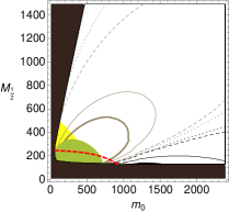
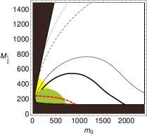
The first factor on the right hand side comes from the phase of which is equal to . Now, from Eq. (51), it is clear that a change in the phase, , would require and a sizeable phase . This fact has strong implications on the size and phases of the mass insertions appearing above. These mass insertions differ in different variations of our model, for instance, that largest MIs can be expected in RVV2. In this model, the mass insertions are and , as one can find in Eqs. (34). The size of the RR insertion depends on and taking for example, we have . These values appear to be large enough to make a significant change in the phase from the second term of Eq. (55). Moreover, the product of these two insertions can have an phase. Notice that this is possible only in RVV2 where the leading terms in these mass insertions have phases. In Fig. 3, we show the different contours of .
Indeed, in model RVV2 there is a region on the plane where it is possible to shift into the interval in Eq. (54), at relatively high and low Dutta:2008xg ; Ko:2008zu .
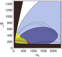
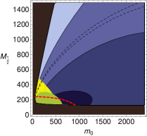
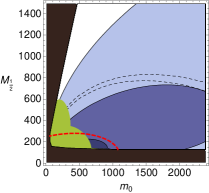
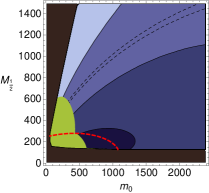
However, these regions of large SUSY contributions to are excluded by LFV and tend to have a too large contribution to as well. If we confine ourselves on a strip allowed by , the maximal value of is around . From the plots we can see that, in the case of RVV1, we are again in the same situation and for the strips allowed by we always have . Although these values could in principle vary due to the unknown coefficients in the soft terms, we can not expect variations in the order of magnitude. Thus, for low and moderate , our models are not able to provide a solution to the anomaly, and, in this situation, we would expect this anomaly to disappear with the inclusion of further data555The authors of Altmannshofer:2009ne claim to be able to satisfy the anomaly and the tension in RVV2. We believe these points correspond to a large value of . Moreover, we checked that the parameters can conspire to give of , even for moderate values of .. If this is the case, our predicted deviation should also be hard to observe at LHCb since it is much smaller than the precision of attainable after 5 years of run (), which is estimated to be phisLHCb .
Similarly, we can repeat a parallel discussion on mixing with the following parameterization,
| (56) |
where each is the same as that in Eqs. (52) with the replacement . The supersymmetric to SM contribution ratio is given by
| (57) |
One can get this result in the same way as for Eq. (55).
In this case, each denominator in the square brackets is smaller than the corresponding one in Eq. (55) by the factor . Again, we use the CKM matrix elements from the full fit by the UTfit collaboration UTfit . In RVV2, we have , and thus we could expect a sizeable effect on if it were not for . However, is suppressed below on an strip in the same way as is. This is below the sensitivity of a super B factory to whose estimate is around Bona:2007qt . In RVV1, the new physics effect is even smaller, since the phases are suppressed. In the end, – mixing is not very much affected in both models. This fact, a posteriori, justifies the way we determine the coefficients in Yukawas: we tune the coefficients so that they reproduce the CKM matrix elements which were obtained under the assumption of no new physics.
Let us come back to the alternative solutions of the puzzle that we mentioned in the previous subsection. If one is to blame the UT fit tension on , one would need a change due to new physics of the amount Lunghi:2008aa . However, this is two orders of magnitude bigger than what can be maximally expected in our models when is at the level of 18%, as we have seen above. In an alternative solution, should be more suppressed, which in turn suppresses as well, thereby making it far less sufficient. The other possibility of invoking modification of does not work for a similar reason. The authors of Ref. Altmannshofer:2009ne need a new physics contribution to this ratio at the level of in order to get an exact agreement. In our models however, the fractional change is about 0.5% at most, which is too small compared to what is needed.
Finally, we can look to the expected values in our model for the decays and that are similar to in the sector. We find that the values of the branching ratios for these processes, in both RVV1 and RVV2 models for and , do not produce deviations from the SM values larger than the per cent level, in spite of the presence of sizeable flavour changing mass insertions. Therefore, these proceses are not interesting tests of new physics in our scenario. This is consistent with the work in Yamada:2007me , where it was found that the deviation from the SM prediction is small once the constraints from and are taken into account.
III.4 Electric Dipole Moments
The EDMs of fermions, such as the electron and the neutron, provide very stringent constraints on CP-violation in new physics. In the SM, the electron EDM from the Kobayashi-Maskawa phase is predicted to be SMeEDM . The SM expectation for the neutron EDM is of SMnEDM , assuming a vanishing . We can see that EDMs are highly suppressed in the SM, and thus they are excellent observables where to look for new physics.
The electron EDM was studied in Calibbi:2008qt within the context of RVV1. In these models CP is spontaneously broken in the flavour sector. Therefore, the phases in the parameter and diagonal terms are very suppressed and can be neglected. In such a case, the imaginary parts required for EDMs only appear from flavour-changing mass insertions Hisano:2008hn . For the electron EDM, only neutralino-mediated diagrams contribute. The most important contribution to , when , comes from a bino-mediated diagram proportional to , which is enhanced by .
In this work, we have updated our analysis on the electron EDM, taking into account the constraints on the and phases imposed by the fit of CKM matrix and the coefficients in (see the Appendix for details). The results are shown for the RVV1 and RVV2 models in Figure 4. An inspection of the slepton soft mass matrices indicates that, for RVV1, the leading phases in the product cancel and only subleading phases contribute, while RVV2 has non-vanishing leading phases. We then have the following predictions:
| (58) | |||||
| (59) |
In Figure 4 we present the sensitivity of current Regan:2002ta and future Lamoreaux:2001hb ; FuteEDM experiments, for the two models. In this Figure, current constraints do not impose any restrictions on the parameter space of either RVV1 or RVV2. Nevertheless, electron EDM predictions are large enough to be probed at future EDM experiments. For relatively light SUSY masses we obtain and , for RVV1 and RVV2, respectively. The latter predicts a value of about one order of magnitude larger than the former for any particular value of and due to the larger suppresion as seen in Eq. (58). This means that by reaching one could probe a much larger part of the evaluated parameter space, with GeV, GeV. In particular, for RVV2, observation of SUSY at the LHC and solving the tension would force to be larger than . However, we have to take into account that these values will vary by factors because of the unknown coefficients to the different MIs.
We now turn to the neutron EDM, . In this observable we have an additional difficulty, since its calculation as a function of partonic EDMs is not straightforward. Here we use two different approaches to this problem, the quark-parton Ellis:1996dg and chiral quark Manohar:1983md models for .
In the quark-parton model Ellis:1996dg , is expressed in terms of the up, down and strange quark EDMs, weighed by the fractional contribution of each quark to the spin of the neutron:
| (60) |
where is a QCD correction factor Degrassi:2005zd and typical values for are , and .
The chiral quark model Manohar:1983md uses naive dimensional analysis to establish:
| (61) |
where is the Wilson coefficient of the EDM operator at the hadronic scale. differs from , which is calculated at the SUSY-breaking scale, since the former receives contributions from the quark chromo-electric dipole moment, , and Weinberg’s gluonic dimension-six operator, Arnowitt:1990eh ; Weinberg:1989dx :
| (62) |
These contributions arise from the operator mixing ocurring in the running from the electroweak scale to the hadronic scale. In our estimates, we take the QCD correction factor Arnowitt:1990eh , and ignore , since it can be at most of the same order of and and we do not expect it to make big changes in our order of magnitude prediction.
The (C)EDM of each quark has contributions from diagrams with gluinos , charginos and neutralinos . For gluinos and neutralinos, we can use the same arguments as in Calibbi:2008qt to establish that the main part of each contribution will come from insertions. Chargino contributions come from both pure higgsino and wino-higgsino diagrams. The mixed wino-higgsino diagrams require no LR flip on the squark line. Contrary to the case with leptons, it is possible to have only one insertion, provided that the CKM matrix element is not flavour-diagonal. For instance, the largest contributions to the down quark (C)EDM are proportional to . Pure higgsino diagrams require a LR flip on the squark line. One would expect this contribution to be strongly suppressed, as there are two Yukawa couplings on the vertices. However, it is possible to exchange one of the small Yukawa couplings for a or coupling through a CKM off-diagonal term. As an example, the main contribution to the pure higgsino diagram for is proportional to . Given the flavour structure of the models, we find that the pure higgsino part shall be larger than the mixed wino-higgsino part, and will dominate the chargino contribution to .
It was noticed in Hisano:2006mj that, in addition to these contributions, it is important to consider beyond-leading-order (BLO) effects. These effects can be represented as new complex effective couplings Buras:2002vd , and although these are noticeable mainly for large values of , for EDMs they can also give significant contributions for moderate and small values of . In particular, diagrams with no imaginary part at LO can become complex from these effective vertices Hisano:2008hn .
The most important BLO effect for the down quark EDM, for the values of we are using, has been found to be the contribution Hisano:2008hn . Although the BLO corrections also affect the gluino, neutralino, chargino and neutral Higgs loops, these contributions represent only small corrections and do not play an important role. Therefore, the only BLO effects we shall include will come from the diagrams.
The BLO effects can also enhance the coupling between the and fermions. At LO, the flavour suppression for an -mediated dipole operator would be of order . The BLO vertex allows us to change the term for a term, having then a total flavour suppression of order . This is comparable to the gluino flavour suppression at LO.
Even though the flavour suppression of the BLO contribution is of an order of magnitude comparable to the LO gluino contribution, the question that needs to be answered is how much does the extra loop suppression affect the diagram. This calculation has been done in Hisano:2006mj , for equal SUSY masses and moderate , giving:
| (63) |
The first square bracket gives a factor of , which is compensated by the loop function , which is of . The third bracket is the flavour suppression ratio, which is of . Thus, in this approximation, the importance of the contribution with respect to the gluino contribution depends mainly on the ratio between the squark and charged Higgs masses squared. Higgs bosons decouple differently from squarks and gauginos, as gluino and squark masses increase faster than the mass for increasing and , the BLO contributions shall be more important for large values of these parameters.
We shall include the contribution through the mass-insertion formulae of Hisano:2008hn . Such an approach contemplates three types of contributions. Two of them involve the CKM matrix, and are of the type and . The third one is similar to that for the gluino loops: . The latter two shall be the ones that will allow us to avoid the suppression. The second term shall be particularly important for RVV1, where the gluino contribution has a cancellation between and .
The predictions for and are shown in Figure 5 for the quark-parton and chiral quark EDMs, respectively. The EDMs receive a significant contribution from the loop in . Furthermore, is also dominated by gluino and contributions to , while is influenced by their contribution to , for both RVV1 and RVV2. The other contributions are smaller by at least half an order of magnitude. We can see that current bounds are always weaker than the LEP and LFV constraints and do not appear in the Figure.
The observation of in the near-future experiments is not always compatible with the solution of the tension. In RVV1, which is mostly dominated by the loops, a of order is usually favoured, one order of magnitude under the reach of the next experiments FutnEDM . In RVV2, both gluino and effects are comparable, the former dominating in the chiral-quark and the latter in the quark-parton models. In both situations it is possible to obtain an observable which is compatible with the solution of the tension.
It is interesting to see that in some regions of the parameter space we have a cancellation. A careful analysis proves that close to these regions the phase of the term vanishes, and that can only be due to a cancellation between the initial term at and the contributions from the running. This causes a change of sign in the gluino contribution, such that it can interfere destructively with the part. We can avoid the cancellations by changing the sign of the terms at , in which case the interference is constructive. This, of course, will turn the cancellation into a small enhancement, but in any case, never exceeds its current bounds.
Finally, Figure 6 shows the same information for . In this situation, the inclusion of the off-diagonal terms allow contributions of the type and . These are always proportional to , although they do not receive a enhancement. It was shown in Calibbi:2008qt that these terms could be important, but they at most remained within the order of magnitude of the terms. Notice that for the insertions are of no interest: although RGE effects can make the off-diagonal terms as large as the terms, they will usually enter the observables accompanied by a or insertion, which are proportional to powers of .
An important contribution that appears when comes from flavour-diagonal subleading phases in . Although the rotation to the SCKM basis removes the leading phases in the flavour-diagonal elements of the trilinear couplings, the different terms makes it impossible to remove the subleading phases in these terms. These phases are suppressed, but they still give important contributions, especially in RVV1, where the leading phases in the contributions from off-diagonal terms cancel. Such an effect is enhanced by the RGE evolution, and is particuarly relevant for the squark sector.
In Figure 6 we can see that, barring the cancellations of the mass-insertion phases, both quark-parton and chiral quark EDMs are similar in magnitude. Although both RVV1 and RVV2 are still not constrained by current bounds, the magnitude of the within the strip is now larger by an order of magnitude, enough to be observed in the near future. The main reason for the similarity in the order of magnitude between models lies in an enhancement of the gluino contribution, due to the subleading phase mentioned in the previous paragraph. For RVV2, this contribution mostly presents a correction to the off-diagonal contributions, but for RVV1 it becomes the main source for .
IV Combined Analysis in the SUSY Parameter Space
In this Section, we are going to present the results of a combined analysis of the observables studied in the previous sections. In particular, we will show the predictions of the model for LFV decays and EDMs in the regions of the parameter space where the SUSY contribution to can account for the possible tension between the measured value and the SM prediction, as discussed in Buras:2008nn . Such a requirement, and always up to possible variations of coefficients, is fulfilled in a restricted portion of the parameter space and allows, as we will see, to do quite definite predictions for the other flavour observables. If we require in addition that the discrepancy between SM and data is explained by SUSY, we are restricted in a region of rather light SUSY masses, where most of the observables are expected to be close to the present experimental bounds. Given both the presence of unknown coefficients and the large theoretical uncertainties in the calculation which don’t allow us to speak of a real failure of the SM, we cannot take what outlined above too seriously. Nevertheless, we think this can be a useful exercise in order to show how the interplay of various flavour observables can be used for testing this kind of flavour models.
In order to understand the impact of the coefficients, in the following plots we shall set all of the s in the soft mass matrices equal to unity. The s of the trilinears shall be kept random, but fixed, since setting them to one aligns them with the Yukawas. At the end of this section we analyze the impact of varying the coefficients, in order to understand how much they affect our correlations.
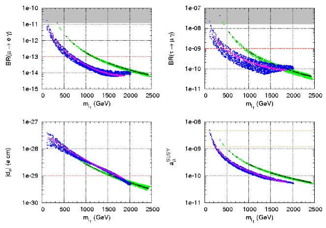
As explained in Section III.2, the SUSY contribution to depends on the sign of the coefficient of the entry , since a negative sign can induce a partial cancellation between the contributions proportional to and . Therefore, we have to take into account both the possible signs for . In Fig. 7, we show the leptonic observables as functions of the lightest slepton mass for the model RVV2 with , , TeV, TeV. The green band corresponds to the points of the parameter space for which , where we have checked that the correct sign has been obtained. For the SM contribution we took the central value computed in Buras:2009pj , , and is the corresponding theoretical error, . The blue band represents the same for the case of negative . The black and purple strips correspond to the more strict requirement , with being the experimental error, (in other words for the strips we assume to take precisely to the central value in Buras:2009pj ). The shaded regions are ruled out by experiment, and the red lines indicate the future experimental sensitivity. For , the area between the yellow lines solve the tension below 2.
The leptonic predictions in these “-favoured” regions are quite interesting. We see that (top-left panel) gives at present practically no constraint, while the final MEG sensitivity (), will test the model up to slepton masses around 0.5-1.2 TeV. Very interestingly, the sensitivity of a Super Flavour Factory reaching can be rather similar (top-right panel). The reason for this is that the “-favoured” region selects rather low values of , where the future bounds of MEG and the Super Flavour Factory are comparable (see Fig. 1 in Section III.1). Concerning eEDM (bottom-left panel), we see that reaching would test this case up to TeV, well beyond the reach of the LFV experiments. Finally, requiring that the SUSY contribution to (bottom-right panel) lowers the tension with the experiments below 2, a rather light spectrum is selected, GeV, so that all the other observables should be in the reach of running/future experiments, with, in particular, branching ratios of LFV decays being just below the present experimental limits.
We checked that model RVV1 gives results for LFV decays and which are similar to the ones of RVV2, while is suppressed by approximately one order of magnitude: in this case, the future sensitivity on will test the parameter space up to slepton masses around 500-750 GeV.
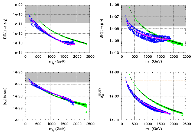
The predictions of Fig. 7 are rather stable also for . In this case, both for RVV1 and RVV2, only and gets slightly increased. For larger values of () we expect, both for RVV1 and RVV2, the future sensitivities for LFV decays and to completely test the parameter space in the range of parameters we considered, TeV, TeV. This is shown in Fig. 8 for RVV2. Notice that, also in this case, it is possible to account for the and the discrepancies at the same time, even if the leptonic observables are in general predicted to be very close to the present experimental bounds.
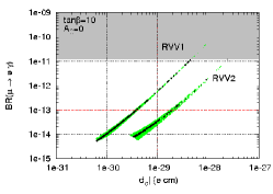
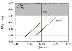
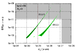
In Fig. 9, we compare the discovery potential of the two most promising leptonic observables, and the electron EDM. The correlation of vs. is plotted for both RVV1 and RVV2, in the case , (left), , (center) and , (right). As before we studied the mass range: TeV, TeV. In the figures, only the “-favoured” region with positive has been plotted. The horizontal line corresponds to the final sensitivity of MEG, the vertical line to the sensitivity on of the running Yale-PdO experiment. We see that, for RVV1, should be able to constrain the parameter space more strongly than eEDM, while for RVV2 it is the most sensitive observable (except for the large case). These features could be useful in the future, in order to discriminate among different models and, more in general, shed light on the structure of mixings and phases in the slepton mass matrix.
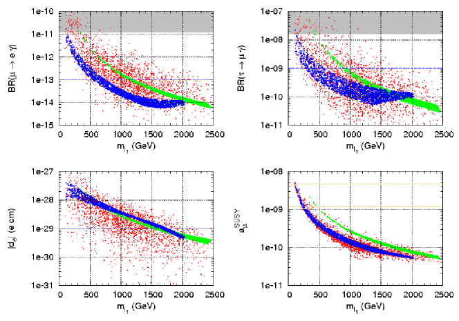
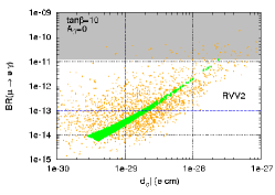
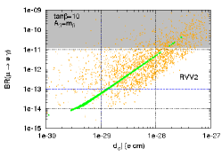
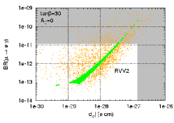
Finally, let us briefly comment about the impact of the unknown coefficients on the analysis outlined above. In Fig. 10, we plot the same observables of Fig. 7 (RVV2, , ) in red, performing a random variation of all the O(1) coefficients between 0.5 and 2 (in absolute value). For comparison, we superimpose to the scatter plot the green and blue bands of Fig. 7. We do the same for Fig. 9 in Fig. 11, only for RVV2, in yellow, superimposing the green bands.
From these Figures we see that, although the lines are broadened by the variation of s, as expected, the correlations are roughly mantained. In some cases we can see variations of even several orders of magnitude for the predictions. This is due to two different sources. On one hand, for fixed values of and we can have a variation of a factor 4 or in the product of two sleptonic coefficients. On the other hand, if we allow the variation of coefficients in , the lines in the (, ) plane of Figure 2 become broad bands, increasing in turn the width of the bands of the sleptonic observables. Still, our predictions remain stable enough, especially for some observables such as , to conclude that the main qualitative features discussed above are not affected too much by the unknown O(1) coefficients.
V Conclusions
In this work, we have studied the phenomenology of a MSSM with a flavour symmetry and spontaneous CP violation. We have shown that in this framework it is possible to fit the observed fermionic masses and mixings simultaneously solving the so-called SUSY flavour and CP problems. As a proof of existence, we have analyzed an explicit example based in the model of Ross, Velasco and Vives Ross:2004qn that successfully overcomes the present FCNC and CP-violation constraints. At the same time, this model predicts a non-trivial flavour structure in the SUSY soft-breaking terms that will show up in near-future CP-violation, LFV and hadronic FCNC experiments. We have analyzed a model that includes the minimal set of contributions to the soft-breaking terms and we have presented two possible variations with additional contributions to soft-breaking terms.
In these models, we naturally expect to be able to observe the decay at MEG for sfermion masses within LHC reach. Similarly, it is also possible to measure the branching ratio at the future Super Flavour Factory. In the hadronic sector the main effect of the model is a sizeable contribution to that could explain the recently observed discrepancy between the SM and the measured value taking the latest lattice values for the factor Buras:2009pj . The electric dipole moment of the electron is also probably to be within reach of the present experiments while the neutron EDM will be just beyond the planned sensitivity of the experiments. It is unfortunate that, at low and without any conspiration of parameters, the evaluated versions of this model cannot provide the required contribution to in order to solve the discrepancy reported in Bona:2008jn . This means that if the future data confirms the discrepancy, non-minimal versions of the model shall be required.
We have made a combined analysis of all the observables if we require that the discrepancy is solved by the SUSY contributions of the model. In this case we are able to relate the values of the different observables and again , and can be measured in the future experiments if SUSY is to be found at LHC.
Acknowledgements.
We would like to thank G. G. Ross, I. de Medeiros Varzielas and M. Passera for useful discussions. L. C. wishes to thank the University of Valencia for the kind hospitality and partial support during various stages of this work. J. J. P. thanks the universities of Padova and Würzburg for hospitality during his visits to complete this work. A. M., J.-h. P. and O. V. would like to thank the Yukawa Institute, Kyoto and the research project YKIS for providing the opportunity to develop an important part of this work in a stimulating and active environment. We acknowledge support from the MEC-INFN agreements FPA2008-04065-E and INFN2008-016. The work of O. V. and J. J. P. was supported by the Spanish MICINN and FEDER (EC) Grant No. FPA2008-02878. O. V. was supported in part by European program MRTN-CT-2006-035482 “Flavianet” and the Generalitat Valenciana under the grant PROMETEO/2008/004. A. M. acknowledges partial support from the CARIPARO Project of Excellence (LHCosmology). W. P. is partially supported by the German Ministry of Education and Research (BMBF) under contract 05HT6WWA. J.-h. P. acknowledges Research Grants funded jointly by the Italian Ministero dell’Istruzione, dell’Università e della Ricerca (MIUR), by the University of Padova and by INFN within the Astroparticle Physics Project. A. M. and W. P. are partially supported by MRTN-CT-2006-035505 (Hep-Tools). A. M. and J.-h. P. acknowledge partial support from the INFN FA51 Grant and from the RTN European Contracts MRTN-CT-2006-035863 (UniverseNet).Appendix A CKM Fit
The model generates the following leading structure for the Yukawa matrices, in terms of and :
| (67) | |||
| (71) |
where . It is necessary to fix the values for the parameters and the flavon phases. In the quark sector, this means that we need to reproduce the quark masses and CKM matrix and, in fact, we will see that the CKM matrix is the main source of constraints on and .
After diagonalizing the Yukawas, keeping terms up to order , and , and rephasing fields such that , , , and are real, we get the following CKM matrix:
| (72) |
where are complex corrections due to subleading terms, with effective phase . These subleading terms play a very important role in the CKM phase which consists on a combination of subleading phases, the largest of these being :
| (73) | |||||
followed by :
| (74) |
Other coefficients are and do not play an important role in the fit. However, it is important to point out that the structure of these subleading terms is highly model dependent, and that the values we get for them shall be valid only in this model. Other models can have a completely different subleading structure.
The phenomenological fit of Roberts:2001zy , based on structures similar to those in Eq. (67), was used in previous works Ross:2004qn ; Calibbi:2008qt to fix the parameters of the Yukawa matrices. In this work we make a new fit specifically for the model, taking into account also flavon phases. Although the variation of the latter make very small changes in the CKM elements, such variations could make these elements exceed the bounds in Amsler:2008zzb .
The values found in Amsler:2008zzb for the CKM matrix are connected to a large number of flavour observables. The analysis assumes that the SM is the only source of flavour and CP violation. Nonetheless, the strong consistency in the SM between all flavour observables, in particular those participating in the construction of the unitarity triangle, suggests that new physics effects are small, and that the main source of the registered flavour and CP violation still lies in the CKM matrix. Thus, we shall adjust the parameters in and such that the CKM matrix of Amsler:2008zzb is reproduced, assuming that SUSY contributions do not affect the fit significantly.
To make a fit of the 11-dimensional parameter space of Eq. (67), the Powell minimization method was used. The function to minimize was defined as a on the quark masses and on the four CKM parameters in the Wolfenstein parametrization: , , and , as in Amsler:2008zzb . We required the parameters not to be larger than 2, and not smaller than . We found that the following values give a very good fit on the masses and mixings:
| (75m) | ||||||
| (75n) | ||||||
with , and non-uniquely determined. The results for are similar to those in Roberts:2001zy , with a larger discrepancy in . The value of is mainly fixed by the CKM phase and , as reported in Ross:2004qn . To leading order, we can extract a uncertainty on the constants from the errors on the CKM parameters Amsler:2008zzb . We roughly expect , and . As the parameters participate only in subleading terms, such a rough estimation is not possible. However, by fixing these constants at the above values, we can estimate the uncertainty on , being .
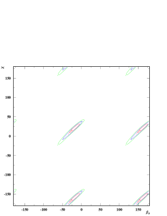
After fixing the determined s at these values, and taking , we make a grid-based analysis on the remaining three phases. We find out that the CKM matrix is completely independent of , as expected from Eq. (72). The result of the scan for and is shown in Figure 12. These two phases enter through subleading terms in the CKM matrix, and are severly constrained due to the precise determination of , and the diagonal elements. We are thus forced to place around , or on any of four degenerate spots obtained by adding to each. For definiteness, in the following we set , and .
Using these values, we compare the results of the fit with the measured values for the CKM matrix and quark masses at Dorsner:2006hw . The results are shown in Tables 7 and 8. We can see that the fit is very good and almost all of the SM parameters lie within their values.
| (GeV) | ||||||
| Reference (GeV) |
| Reference |
|---|
Regarding the lepton sector, we shall unify the structure of quark and lepton flavoured matrices, so the Yukawas can be written as:
| (79) | |||
| (83) |
with and and . Notice that in the zeroes are actually terms of order higher than . We use the same s in for and we find that the s that fit best the charged lepton masses are:
| (84) |
which give the values in Table 9. Note that lepton masses are known very precisely and thus subleading contributions will play an important role in the fit. For this reason, we did not try to fit exactly the reference values in Table 9.
For more details on how the model accomodates neutrino mixing, we refer the interested reader to Ross:2004qn .
| (GeV) | |||
|---|---|---|---|
| Reference (GeV) |
Appendix B Coefficients in the SCKM Basis at the GUT Scale
In general, flavour symmetry models contain unknown coefficients at the flavour scale. In CPV and FCNC studies we are interested in the leading real and imaginary contributions. However, we find that in some particular observables, leading phases might cancel. In such a situation it is important to know the structure of subleading complex terms in order to make verifiable predictions. For this purpose, we present here the structure of the coefficients for the leading terms after the SCKM rotation.
In the following, we shall define , with .
B.1 RVV1
Our soft matrices in the flavour basis have the following structure at the GUT scale:
with exactly the same structure, but different constants and , for and , respectively. For and we have an analogous structure, with replaced by , replaced by , and different constants and . This shall be true for all variations of the model, so in following subsections we shall only show without repeating these specifications.
Rotation into the SCKM basis gives Eq (32), with the following coefficients:
| (85a) | |||||
| (85b) | |||||
| (85c) | |||||
| (86a) | |||||
| (86b) | |||||
| (86c) | |||||
| (87a) | |||||
| (87b) | |||||
| (87c) | |||||
| (88a) | |||||
| (88b) | |||||
| (88c) | |||||
| (89a) | |||||
| (89b) | |||||
| (89c) | |||||
B.2 RVV2
The Kähler potential in RVV2 has got the minimal terms with the addition of the flavon vevs. This modifies the and elements of the soft mass matrices, giving them the following structure at the GUT scale:
For simplicity, we have omitted the minimal () s, replacing them by the corresponding that accompany the flavon vev. The coefficients are:
| (90a) | |||||
| (90b) | |||||
| (90c) | |||||
| (91a) | |||||
| (91b) | |||||
| (91c) | |||||
| (92a) | |||||
| (92b) | |||||
| (92c) | |||||
| (93a) | |||||
| (93b) | |||||
| (93c) | |||||
| (94a) | |||||
| (94b) | |||||
| (94c) | |||||
B.3 RVV Model 3
The addition of an effective term with the antisymmetric flavon vevs gives the soft matrices the following structure, in the flavour basis, at the GUT scale:
The additional term in the and sectors of the mass matrices induce large terms in the and sectors of the mass matrices, and have a moderate influence on the and sectors. The structure of the coefficients follow:
| (95a) | |||||
| (95b) | |||||
| (95c) | |||||
| (96a) | |||||
| (96b) | |||||
| (96c) | |||||
| (97a) | |||||
| (97b) | |||||
| (97c) | |||||
| (98a) | |||||
| (98b) | |||||
| (98c) | |||||
| (99a) | |||||
| (99b) | |||||
| (99c) | |||||
B.4 A-Terms
For all of the evaluated models, the A-Terms will have the same structure the Yukawas have, but with different constants. We parametrize them in the following way:
| (100) |
and similarly for and .
The A-Terms are rotated into the SCKM basis using the same unitary matrices that diagonalize the Yukawas. However, as the constants in each entry are different from the ones in the Yukawas, the A-Terms are not diagonalized, and mantain the same structure. For squarks, the remaining off-diagonal terms are then affected by the rephasings, and we obtain:
| (104) | |||
| (108) | |||
| (112) |
with:
| (113a) | |||||
| (113b) | |||||
| (113c) | |||||
with no subleading phases generated by the SCKM rotation. Notice that if the initial , the A-terms are aligned with the Yukawas. Thus, the new go to zero, and the A-terms are diagonal at the SCKM basis.
Appendix C O(1) Constants due to RGEs
Using the leading log approximation, we can estimate the effect of the running on the flavoured matrices. For this we define the negative parameter , such that:
The rotation to the SCKM basis must be done at . However, since the off-diagonal RGE contributions to the Yukawa matrices are negligible, we can perform the rotation at the GUT scale, and then apply the corrections from the running.
For , one must take into account that only the term of gives a significant contribution to the running. This parameter only participates until the heavy decouples, at the scale . To take into account this effect, we introduce the parameter:
With the exception of the A-Terms, the general result for all models is that the structure in terms of and remains unchanged. Even though the generated parameters are not necessarily of , the parameter provides an additional suppression, which approximately keeps the matrix structure very similar to the one at the GUT scale.
These induced coefficients can have two parts: one independent of the flavour structure of the soft masses (the MFV contribution, generated by the misalignment of the Yukawa matrices), and one dependent on the flavour structure. In the following equations, those parts independent of the soft mass flavour structure can be distinguished because they do not vanish when the terms () are set to zero and when the terms are set to one (this also sets all primed variables to zero). They are only present in the , and matrices.
In the following, we shall denote , at the scale , as , with . For all soft mass terms, we shall factorize the and factors that appear in the mass matrices presented in Eq. (32), as well as the leading phase. Since we shall also factorize , we define .
C.1 RVV Model 1
| (114a) | |||||
| (114b) | |||||
| (114c) | |||||
| (115a) | |||||
| (115b) | |||||
| (115c) | |||||
| (116a) | |||||
| (116b) | |||||
| (116c) | |||||
| (117a) | |||||
| (117b) | |||||
| (117c) | |||||
| (118a) | |||||
| (118b) | |||||
| (118c) | |||||
C.2 RVV Model 2
| (119a) | |||||
| (119b) | |||||
| (119c) | |||||
| (120a) | |||||
| (120b) | |||||
| (120c) | |||||
| (121a) | |||||
| (122a) | |||||
| (122b) | |||||
| (122c) | |||||
| (123a) | |||||
C.3 RVV Model 3
| (124a) | |||||
| (124b) | |||||
| (124c) | |||||
| (125a) | |||||
| (125b) | |||||
| (125c) | |||||
| (126a) | |||||
| (126b) | |||||
| (127a) | |||||
| (127b) | |||||
| (127c) | |||||
| (128a) | |||||
| (128b) | |||||
| (128c) | |||||
C.4 A-Terms
To write the RGE contribution for the A-Terms, we shall first denote:
| (129a) | |||||
| (129b) | |||||
| (129c) | |||||
| (129d) | |||||
| (129e) | |||||
| (129f) | |||||
As the A-Terms are not hermitian matrices, the RGE evolution is different for each off-diagonal term. For each element, we shall factorize in Eq. (104) the leading order of magnitude in terms of or , the phase, and the global term . Then, after the running, we get:
| (130a) | |||||
| (130b) | |||||
| (130c) | |||||
| (130d) | |||||
| (130e) | |||||
| (130f) | |||||
| (130g) | |||||
| (130h) | |||||
| (130i) | |||||
| (131a) | |||||
| (131b) | |||||
| (131c) | |||||
| (131d) | |||||
| (131e) | |||||
| (131f) | |||||
| (131g) | |||||
| (131h) | |||||
| (131i) | |||||
with:
| (132a) | |||||
| (132b) | |||||
| (132c) | |||||
| (132d) | |||||
We see that the running can generate subleading phases, which are contained within the terms. In particular, it is noticeable that these phases do not vanish when aligning the A-Terms with the Yukawas (setting all ), which means they belong to a MFV contribution.
It is also important to remark the fact that and contain terms of order and , which are enhancement factors. Again, these are due to MFV contributions. Thus, the RGE evolution has the potential of changing the structure of noticeably.
We do not list the matrices, since their structure is identical to , with the replacements , , , and . One must also consider and .
References
- (1) A. Masiero and O. Vives, Ann. Rev. Nucl. Part. Sci. 51 (2001) 161 [arXiv:hep-ph/0104027].
- (2) A. Masiero, S. K. Vempati and O. Vives, arXiv:0711.2903 [hep-ph].
- (3) G. G. Ross, L. Velasco-Sevilla and O. Vives, Nucl. Phys. B 692, 50 (2004) [arXiv:hep-ph/0401064]
- (4) L. Calibbi, J. Jones-Perez and O. Vives, Phys. Rev. D 78 (2008) 075007 [arXiv:0804.4620 [hep-ph]].
- (5) C. D. Froggatt and H. B. Nielsen, Nucl. Phys. B 147 (1979) 277.
- (6) M. Leurer, Y. Nir and N. Seiberg, Nucl. Phys. B 398 (1993) 319 [arXiv:hep-ph/9212278].
- (7) A. Pomarol and D. Tommasini, Nucl. Phys. B 466, 3 (1996) [arXiv:hep-ph/9507462].
- (8) P. Binetruy, S. Lavignac and P. Ramond, Nucl. Phys. B 477 (1996) 353 [arXiv:hep-ph/9601243].
- (9) E. Dudas, C. Grojean, S. Pokorski and C. A. Savoy, Nucl. Phys. B 481, 85 (1996) [arXiv:hep-ph/9606383].
- (10) H. K. Dreiner, H. Murayama and M. Thormeier, Nucl. Phys. B 729 (2005) 278 [arXiv:hep-ph/0312012].
- (11) G. L. Kane, S. F. King, I. N. R. Peddie and L. Velasco-Sevilla, JHEP 0508 (2005) 083 [arXiv:hep-ph/0504038].
- (12) P. H. Chankowski, K. Kowalska, S. Lavignac and S. Pokorski, Phys. Rev. D 71 (2005) 055004 [arXiv:hep-ph/0501071].
- (13) R. Barbieri, G. R. Dvali and L. J. Hall, Phys. Lett. B 377, 76 (1996) [arXiv:hep-ph/9512388].
- (14) R. Barbieri, L. J. Hall, S. Raby and A. Romanino, Nucl. Phys. B 493, 3 (1997) [arXiv:hep-ph/9610449].
- (15) S. F. King and G. G. Ross, Phys. Lett. B 520, 243 (2001) [arxiv:hep-ph/0108112]
- (16) S. F. King and G. G. Ross, Phys. Lett. B 574, 239 (2003) [arxiv:hep-ph/0307190]
- (17) I. de Medeiros Varzielas and G. G. Ross, Nucl. Phys. B 733 (2006) 31 [arXiv:hep-ph/0507176].
- (18) I. de Medeiros Varzielas, S. F. King and G. G. Ross, Phys. Lett. B 644 (2007) 153 [arXiv:hep-ph/0512313].
- (19) I. de Medeiros Varzielas, S. F. King and G. G. Ross, Phys. Lett. B 648 (2007) 201 [arXiv:hep-ph/0607045].
- (20) T. Kobayashi, H. P. Nilles, F. Ploger, S. Raby and M. Ratz, Nucl. Phys. B 768 (2007) 135 [arXiv:hep-ph/0611020].
- (21) H. Ishimori, T. Kobayashi, H. Okada, Y. Shimizu and M. Tanimoto, JHEP 0904 (2009) 011 [arXiv:0811.4683 [hep-ph]].
- (22) H. Ishimori, T. Kobayashi, H. Okada, Y. Shimizu and M. Tanimoto, arXiv:0907.2006 [hep-ph].
- (23) G. Altarelli and F. Feruglio, Nucl. Phys. B 720 (2005) 64 [arXiv:hep-ph/0504165].
- (24) T. Kobayashi, Y. Omura and K. Yoshioka, Phys. Rev. D 78 (2008) 115006 [arXiv:0809.3064 [hep-ph]].
- (25) G. Seidl, arXiv:0811.3775 [hep-ph].
- (26) G. G. Ross and O. Vives, Phys. Rev. D 67, 095013 (2003) [arXiv:hep-ph/0211279]
- (27) S. Antusch, S. F. King and M. Malinsky, arXiv:0708.1282 [hep-ph].
- (28) K. A. Olive and L. Velasco-Sevilla, arXiv:0801.0428 [hep-ph].
- (29) G. G. Ross and L. Velasco-Sevilla, Nucl. Phys. B 653 (2003) 3 [arXiv:hep-ph/0208218].
- (30) F. Gabbiani, E. Gabrielli, A. Masiero and L. Silvestrini, Nucl. Phys. B 477 (1996) 321 [arXiv:hep-ph/9604387].
- (31) J. S. Hagelin, S. Kelley and T. Tanaka, Nucl. Phys. B 415 (1994) 293.
- (32) F. Borzumati and A. Masiero, Phys. Rev. Lett. 57 (1986) 961
- (33) J. A. Casas and A. Ibarra, Nucl. Phys. B 618, 171 (2001) [arXiv:hep-ph/0103065].
- (34) A. Masiero, S. K. Vempati and O. Vives, Nucl. Phys. B 649, 189 (2003) [arXiv:hep-ph/0209303].
- (35) W. Porod, Comput. Phys. Commun. 153 (2003) 275 [arXiv:hep-ph/0301101].
- (36) R. G. Roberts, A. Romanino, G. G. Ross and L. Velasco-Sevilla, Nucl. Phys. B 615 (2001) 358 [arXiv:hep-ph/0104088].
- (37) C. Amsler et al. [Particle Data Group], Phys. Lett. B 667, 1 (2008).
- (38) R. Barate et al. [LEP Working Group for Higgs boson searches and ALEPH Collaboration and and], Phys. Lett. B 565 (2003) 61 [arXiv:hep-ex/0306033].
- (39) A. Djouadi, M. Drees and J. L. Kneur, JHEP 0108 (2001) 055 [arXiv:hep-ph/0107316].
- (40) B. C. Allanach, A. Djouadi, J. L. Kneur, W. Porod and P. Slavich, JHEP 0409, 044 (2004) [arXiv:hep-ph/0406166].
- (41) S. Heinemeyer, W. Hollik, H. Rzehak and G. Weiglein, Eur. Phys. J. C 39 (2005) 465 [arXiv:hep-ph/0411114].
- (42) S. Chen et al. [CLEO Collaboration], Phys. Rev. Lett. 87 (2001) 251807 [arXiv:hep-ex/0108032].
- (43) Belle Collaboration, talk by A. Limosani at Moriond EW (2008)
- (44) B. Aubert et al. [BABAR Collaboration], Phys. Rev. D 72 (2005) 052004 [arXiv:hep-ex/0508004].
- (45) Heavy Flavor Averaging Group web page: http://www.slac.stanford.edu/xorg/hfag/
- (46) T. Hurth, E. Lunghi and W. Porod, Nucl. Phys. B 704 (2005) 56 [arXiv:hep-ph/0312260].
- (47) G. Degrassi, P. Gambino and P. Slavich, Comput. Phys. Commun. 179 (2008) 759 [arXiv:0712.3265 [hep-ph]].
- (48) T. Becher and M. Neubert, Phys. Rev. Lett. 98 (2007) 022003 [arXiv:hep-ph/0610067].
- (49) E. Lunghi and J. Matias, JHEP 0704 (2007) 058 [arXiv:hep-ph/0612166].
- (50) G. W. Bennett et al. [Muon G-2 Collaboration], Phys. Rev. D 73 (2006) 072003 [arXiv:hep-ex/0602035].
- (51) J. P. Miller, E. de Rafael and B. L. Roberts, Rept. Prog. Phys. 70 (2007) 795 [arXiv:hep-ph/0703049].
- (52) M. Passera, W. J. Marciano and A. Sirlin, Phys. Rev. D 78 (2008) 013009 [arXiv:0804.1142 [hep-ph]].
- (53) F. Jegerlehner and A. Nyffeler, Phys. Rept. 477 (2009) 1 [arXiv:0902.3360 [hep-ph]].
- (54) T. Moroi, Phys. Rev. D 53 (1996) 6565 [Erratum-ibid. D 56 (1997) 4424] [arXiv:hep-ph/9512396].
- (55) M. Davier, S. Eidelman, A. Hocker and Z. Zhang, Eur. Phys. J. C 27 (2003) 497 [arXiv:hep-ph/0208177].
- (56) M. Ahmed et al. [MEGA Collaboration], Phys. Rev. D 65 (2002) 112002 [arXiv:hep-ex/0111030].
- (57) MEG Experiment: http://meg.psi.ch.
- (58) S. Banerjee, Nucl. Phys. Proc. Suppl. 169 (2007) 199 [arxiv:hep-ex/0702017]
- (59) A. Lusiani, [arXiv:0709.1599 [hep-ex]]
- (60) M. Bona et al., arXiv:0709.0451 [hep-ex].
- (61) B. Aubert et al. [BABAR Collaboration], Phys. Rev. Lett. 96 (2006) 041801 [arXiv:hep-ex/0508012].
- (62) A. G. Akeroyd et al. [SuperKEKB Physics Working Group], arXiv:hep-ex/0406071.
- (63) A. J. Buras and D. Guadagnoli, arXiv:0901.2056 [hep-ph].
- (64) A. J. Buras and D. Guadagnoli, Phys. Rev. D 78 (2008) 033005 [arXiv:0805.3887 [hep-ph]].
- (65) D. J. Antonio et al. [RBC Collaboration and UKQCD Collaboration], Phys. Rev. Lett. 100 (2008) 032001 [arXiv:hep-ph/0702042].
- (66) C. Allton et al. [RBC-UKQCD Collaboration], Phys. Rev. D 78 (2008) 114509 [arXiv:0804.0473 [hep-lat]].
- (67) C. Aubin, J. Laiho and R. S. Van de Water, arXiv:0905.3947 [hep-lat].
- (68) E. Lunghi and A. Soni, Phys. Lett. B 666 (2008) 162 [arXiv:0803.4340 [hep-ph]].
- (69) M. Ciuchini et al., JHEP 9810 (1998) 008 [arXiv:hep-ph/9808328].
- (70) Y. Nakamura et al. [CP-PACS Collaboration], PoS LAT2006 (2006) 089 [arXiv:hep-lat/0610075].
- (71) A. J. Buras, G. Colangelo, G. Isidori, A. Romanino and L. Silvestrini, Nucl. Phys. B 566 (2000) 3 [arXiv:hep-ph/9908371].
- (72) Y. Nir and M. P. Worah, Phys. Lett. B 423 (1998) 319 [arXiv:hep-ph/9711215].
- (73) A. J. Buras, A. Romanino and L. Silvestrini, Nucl. Phys. B 520 (1998) 3 [arXiv:hep-ph/9712398].
- (74) G. Colangelo and G. Isidori, JHEP 9809 (1998) 009 [arXiv:hep-ph/9808487].
- (75) M. Bona et al. [UTfit Collaboration], arXiv:0803.0659 [hep-ph].
- (76) E. Barberio et al. [Heavy Flavor Averaging Group], arXiv:0808.1297 [hep-ex].
- (77) D. Becirevic et al., Nucl. Phys. B 634 (2002) 105 [arXiv:hep-ph/0112303].
- (78) G. Buchalla, A. J. Buras and M. E. Lautenbacher, Rev. Mod. Phys. 68 (1996) 1125 [arXiv:hep-ph/9512380].
- (79) UTFit web page: http://www.utfit.org/
- (80) B. Dutta and Y. Mimura, Phys. Rev. D 78 (2008) 071702 [arXiv:0805.2988 [hep-ph]].
- (81) P. Ko, J. h. Park and M. Yamaguchi, JHEP 0811 (2008) 051 [arXiv:0809.2784 [hep-ph]].
- (82) [LHCb Collaboration], Expression of interest for an LHCb upgrade, CERN/LHCC/2008-007.
- (83) W. Altmannshofer, A. J. Buras, S. Gori, P. Paradisi and D. M. Straub, arXiv:0909.1333 [hep-ph].
- (84) Y. Yamada, Phys. Rev. D 77, 014025 (2008) [arXiv:0709.1022 [hep-ph]].
- (85) M. E. Pospelov and I. B. Khriplovich, Sov. J. Nucl. Phys. 53 (1991) 638
- (86) I. B. Khriplovich and A. R. Zhitnitsky, Phys. Lett. B 109 (1982) 490
- (87) J. Hisano, M. Nagai and P. Paradisi, Phys. Lett. B 642 (2006) 510 [arXiv:hep-ph/0606322].
- (88) A. J. Buras, P. H. Chankowski, J. Rosiek and L. Slawianowska, Nucl. Phys. B 659 (2003) 3 [arXiv:hep-ph/0210145].
- (89) J. Hisano, M. Nagai and P. Paradisi, arXiv:0812.4283 [hep-ph].
- (90) B. C. Regan and E. D. Commins and C. J. Schmidt and D. DeMille, Phys. Rev. Lett. 88 (2002) 071805
- (91) S. K. Lamoreaux, [arXiv:nucl-ex/0109014]
-
(92)
Cs and Rb eEDM Experiment: http://www.phys.psu.edu/research/amo/
HfF+ eEDM Experiment: http://jilawww.colorado.edu/bec/index.html
PbO eEDM Experiment: http://www.yale.edu/demillegroup/
YbF eEDM Experiment: http://www3.imperial.ac.uk/ccm/research/edm - (93) J. R. Ellis and R. A. Flores, Phys. Lett. B 377 (1996) 83 [arXiv:hep-ph/9602211].
- (94) A. Manohar and H. Georgi, Nucl. Phys. B 234 (1984) 189.
- (95) G. Degrassi, E. Franco, S. Marchetti and L. Silvestrini, JHEP 0511 (2005) 044 [arXiv:hep-ph/0510137].
- (96) R. L. Arnowitt, J. L. Lopez and D. V. Nanopoulos, Phys. Rev. D 42 (1990) 2423.
- (97) S. Weinberg, Phys. Rev. Lett. 63 (1989) 2333.
-
(98)
CryoEDM Experiment: http://hepwww.rl.ac.uk/EDM/index_files/CryoEDM.htm
PNPI nEDM Experiment: http://nrd.pnpi.spb.ru/LabSereb/neutronedm.htm
PSI nEDM Experiment: http://nedm.web.psi.ch/
SNS nEDM Experiment: http://p25ext.lanl.gov/edm/edm.html - (99) I. Dorsner, P. Fileviez Perez and G. Rodrigo, Phys. Rev. D 75 (2007) 125007 [arXiv:hep-ph/0607208].