Magnetocaloric effect in quantum spin-$s$ chains

Abstract

We compute the entropy of antiferromagnetic quantum spin-$s$ chains in an external magnetic field using exact diagonalization and Quantum Monte Carlo simulations. The magnetocaloric effect, i.e., temperature variations during adiabatic field changes, can be derived from the isentropes. First, we focus on the example of the spin-$s=1$ chain and show that one can cool by closing the Haldane gap with a magnetic field. We then move to quantum spin-$s$ chains and demonstrate linear scaling with $s$ close to the saturation field.

In passing, we propose a new method to compute many low-lying excited states using the Lanczos recursion.

Key words: Quantum spin chains, magnetocaloric effect, entropy, exact diagonalization, Quantum Monte Carlo

PACS: 75.10.Pq; 75.30.Sg; 75.50.Ee; 02.70.-c

1 Introduction

The magnetocaloric effect, i.e., a temperature change induced by an adiabatic change of an external magnetic field was discovered in iron by Warburg in 1881 [1]. This effect also has a long history in cooling applications. For example, adiabatic demagnetization of paramagnetic salts was the first method to reach temperatures below 1K [2]. Among the many experimental but also theoretical investigations to follow, we would like to mention in particular the computation of the field variation of the entropy in a quantum spin-1/2 $XXZ$ chain [3]. This investigation is remarkable in so far as it is one of the very first numerical computations for an interacting quantum many-body system. The relation of the entropy of quantum spin chains in a magnetic field to magnetic cooling was also noted [4] and even one exact computation was performed, albeit for a chain with a strong easy-axis anisotropy [5].

The magnetocaloric effect in quantum spin systems has recently attracted renewed attention. The reason for this is two-fold. On the one hand, field-induced quantum phase transitions lead to universal responses when the applied field is varied adiabatically [6, 7]. On the other hand, it was observed that the magnetocaloric effect is enhanced by geometric frustration [9, 10, 11, 12, 13, 14, 15, 16, 17, 18, 19, 20, 21, 22, 23], promising improved efficiency in low-temperature cooling applications. In this context, the isotropic spin-1/2 Heisenberg chain, the isotropic and anisotropic $XY$ chain in a transverse field [10], and the quantum Ising chain in a transverse field [7] were also revisited. One further example of a non-frustrated quantum spin chain where the magnetocaloric effect was computed is the ferrimagnetic spin-$1$-$5/2$ chain [24]. Finally, the adiabatic cooling rate has recently been measured on the spin-1/2 Heisenberg chain compound [Cu($\mu$-C₂O₄)(4-aminopyridine)₂(H₂O)]_n [25] and relatedly the magnetocaloric effect of the spin-1/2 isotropic Heisenberg and $XXZ$ chains was computed exactly [26].

In this paper we will investigate magnetocaloric properties of quantum spin-$s$ Heisenberg chains given by the Hamiltonians

$$H=J\,\sum_{i=1}^{L}\vec{S}_{i}\cdot\vec{S}_{i+1}-h\,\sum_{i=1}^{L}S_{i}^{z}\,.$$ (1)

$J>0$ is the antiferromagnetic exchange constant, $h$ an external magnetic field, $L$ the length of the chain, and $\vec{S}_{i}$ are quantum spin-$s$ operators at site $i$. We will use periodic boundary conditions, i.e., $\vec{S}_{L+1}=\vec{S}_{1}$.

In section 2 we will first summarize the methods which we are going to use, namely exact diagonalization (ED) and Quantum Monte Carlo (QMC) simulations using the Stochastic Series Expansion (SSE) framework. Then we will apply these methods to the $s=1$ chain in section 3. The spin $s=1$ Heisenberg chain is famous for the presence of the so-called ‘Haldane’ gap at $h=0$ [27, 28, 29, 30]. In particular, we will illustrate with the $s=1$ chain that one can exploit the presence of a spin gap for cooling by adiabatic magnetization at low magnetic fields. Next, we discuss the scaling with spin quantum number $s$ in section 4. In particular, we will show that there is a quantum scaling regime at low temperatures close to the saturation field where one has linear scaling with $s$. Finally, in section 5 we will conclude with a summary.

2 Methods

2.1 Exact diagonalization

Thermodynamic quantities can be computed using spectral representations. For example, the entropy can be written as [10]

$$S=\frac{1}{T\,Z}\sum_{n}E_{n}\,{\rm e}^{-E_{n}/T}+\ln Z\,,$$ (2)

where $Z=\sum_{n}{\rm e}^{-E_{n}/T}$ is the partition function and $E_{n}$ are the eigenvalues of the Hamiltonian.

In order to evaluate spectral representations like (2), one needs to diagonalize the Hamiltonian. If this is done numerically exactly, this is called Exact Diagonalization (ED). First, one should perform a symmetry reduction. We have used translations and $S^{z}$-conservation as well as reflections and spin inversion where appropriate. One can then use a library routine to perform a full diagonalization. Such an approach is very much in the spirit of classic work [3, 31, 32]. The main technical differences of our computations and [3, 31, 32] are: (i) we have exploited $SU(2)$-symmetry to reconstruct the $S^{z}=1$ sector from the $S^{z}\geq 2$ sectors and the spin-inversion resolved $S^{z}=0$ sector, (ii) we have used improved implementations of the diagonalization routines [33, 34], (iii) and we have substantially more powerful computers at our disposal. The combination of these factors enables us to compute full spectra for bigger systems than in the 1960s.

If we are interested only in low-energy properties, we can use iterative diagonalization algorithms like the Lanczos method [35, 36, 37].

The basic Lanczos algorithm [35, 36, 37] for a Hermitian matrix $H$ proceeds as follows. For a given normalized start vector $\vec{v}_{1}$, one defines a sequence of normalized Lanczos vectors $\vec{v}_{j}$ via the recurrence relations

$$\beta_{j+1}\,\vec{v}_{j+1} = H\,\vec{v}_{j}-\alpha_{j}\,\vec{v}_{j}-\beta_{j}\,\vec{v}_{j-1}\,,$$

$$\alpha_{j} = \vec{v}_{j}\cdot H\,\vec{v}_{j}\,,$$ (3)

$$\beta_{j+1} = \vec{v}_{j+1}\cdot H\,\vec{v}_{j}\,,$$

with the initial conditions $\beta_{1}=0$ and $\vec{v}_{0}=\vec{0}$. The real coefficients $\alpha_{i}$ and $\beta_{i}$ define the so-called Lanczos matrices

$$T_{n}=\begin{pmatrix}\alpha_{1}&\beta_{2}&0&\ldots&\ldots&0\\ \beta_{2}&\alpha_{2}&\ddots&\ddots&&\vdots\\ 0&\ddots&\ddots&\ddots&\ddots&\vdots\\ \vdots&\ddots&\ddots&\ddots&\ddots&0\\ \vdots&&\ddots&\ddots&\ddots&\beta_{n}\\ 0&\ldots&\ldots&0&\beta_{n}&\alpha_{n}\end{pmatrix}\,.$$ (4)

The crucial point of the Lanczos algorithm is that the eigenvalues of $T_{n}$ yield a good approximation of the extremal eigenvalues of $H$ already for $n$ much smaller than the total Hilbert space dimension.

The Lanczos algorithm suffers from one practical problem: the recursion relations (3) are supposed to guarantee mutual orthogonality of the vectors $\vec{v}_{i}$, i.e., $\vec{v}_{i}\cdot\vec{v}_{j}=0$ for $i\neq j$. However, this fails to be correct when the computations are carried out numerically, leading to undesired spurious states, called ghost states [36, 37]. Several strategies have been proposed [36, 37] in order to deal with the ghost problem during the computation of excited eigenvalues.

Here we suggest another method to compute excited states with controlled accuracy and correct multiplicity. We start by performing a fixed number $n$ of Lanczos iterations with a given start vector $\vec{v}_{1}$. Next we compute the orthogonal transformation $U_{i,j}$, $1\leq i,j\leq n$ diagonalizing the Lanczos matrix (4). Then we fix a number $m\ll n$ and repeat the Lanczos procedure with the same start vector $\vec{v}_{1}$. During this second Lanczos pass we construct $m$ vectors

$$\vec{u}_{i}=\sum_{j=1}^{n}U_{j,i}\,\vec{v}_{j}\,,\qquad 1\leq i\leq m\,.$$ (5)

The second Lanczos pass is needed in order to avoid storing the $n\gg m$ Lanczos vectors $\vec{v}_{j}$.

The vectors $\vec{u}_{i}$ given by (5) yield approximations to the eigenvectors of $H$. However, due to the ghost problem, there are spurious vectors which need to be eliminated. We perform this in two steps. First, using the observation that the vectors $\vec{u}_{i}$ are supposed to be mutually orthogonal, we can eliminate those $\vec{u}_{i}$ which have big projections on the $\vec{u}_{j}$ with $j<i$. Second, we reorthogonalize the remaining vectors yielding $\tilde{m}\leq m$ orthonormal vectors $\tilde{\vec{u}}_{i}$. Finally, we project the matrix $H$ onto this subspace via

$$H_{i,j}=\tilde{\vec{u}}_{i}\cdot H\,\tilde{\vec{u}}_{j}\,.$$ (6)

A full diagonalization of the $\tilde{m}\times\tilde{m}$ matrix $H_{i,j}$ and application of the resulting basis transformation to the vectors $\tilde{\vec{u}}_{i}$ yields $\tilde{m}$ orthogonal vectors $\vec{w}_{i}$ which approximate the eigenvectors of $H$. The eigenvalues $E_{i}$ associated to the vectors $\vec{w}_{i}$ and their accuracy can be estimated according to

$$E_{i}=\vec{w}_{i}\cdot H\,\vec{w}_{i}\,,\qquad\delta E_{i}^{2}=\vec{w}_{i}\cdot\left(H-E_{i}\right)^{2}\vec{w}_{i}\,.$$ (7)

According to our experience, there are neither any missing nor any spurious eigenvalues among the converged ones. It should be mentioned that there is no guarantee that the Lanczos procedure yields the complete spectrum for a given start vector $\vec{v}_{1}$, in particular if one has not performed a complete symmetry decomposition. Nevertheless, numerical noise seems to prevent this from happening, at least for sufficiently generic start vectors $\vec{v}_{1}$.

For our procedure one needs to choose the number of Lanczos iterations $n$ and the dimension of the subspace $m\leq n$ in advance and the whole procedure needs to be repeated if it turns out that less than the desired number of converged eigenvalues have been obtained. In practice, however, one obtains results of a comparable quality for a class of problems where the choice of $n$ and $m$ has been adjusted for one representative case. In the examples to be reported below, we have been able to obtain about 100 eigenvalues in a given symmetry sector with a relative accuracy of $10^{-8}$ or better using $n=2000$ Lanczos iterations and $m=500$ vectors $\vec{u}_{i}$.

2.2 Quantum Monte Carlo

Since the system sizes accessible by either full diagonalization or Lanczos diagonalization are limited, it is desirable to have other methods at our disposal. For non-frustrated spin models like the spin-$s$ Heisenberg chain (1), one can in principle use Quantum Monte Carlo (QMC) simulations. There is, however, one problem: we are particularly interested in the entropy which is usually obtained with large statistical errors from integrating a Monte-Carlo result for the specific heat. In this subsection we will summarize how one can circumvent this problem.

In order to obtain a QMC estimate of the temperature dependence of the entropy, we employed an extended ensemble, broad-histogram method [38, 39, 40] within the Stochastic Series Expansion (SSE) framework [41, 42, 43, 44]. Based on this approach, thermodynamic quantities can be obtained over a broad range of temperatures from a single QMC simulation that provides estimates of the expansion coefficients $g(n)$ of the system’s partition function $Z$ in a high-temperature series expansion:

$$Z=\mathrm{Tr}\,{\rm e}^{-\beta H}=\sum_{n=0}^{\infty}g(n)\beta^{n}.$$ (8)

Here, $\beta=1/T$ is the inverse temperature. In terms of the expansion coefficients $g(n)$, the internal energy is obtained using

$$E=\langle H\rangle=-\frac{\partial}{\partial\beta}\ln Z=-\frac{1}{Z}\sum_{n}g(n)n\beta^{n-1}=-\frac{1}{\beta}\langle n\rangle,$$ (9)

and the free energy from

$$F=-\frac{1}{\beta}\ln{Z}=-\frac{1}{\beta}\ln\sum_{n}g(n)\beta^{n}.$$ (10)

Finally, the entropy can be calculated using $S=(E-F)/T$.

In the QMC simulation, estimates of the first $\Lambda$ coefficients $g(n),n=0,...,\Lambda$ are obtained by performing a random walk in the expansion order $n$, such as to sample efficiently all expansion orders from $n=0$ (where $g(0)=(2s+1)^{L}$ for a spin-$s$ chain of $L$ sites is known exactly) to $n=\Lambda$. This is accomplished using an extension of the Wang-Landau flat-histogram sampling algorithm [45, 46] to the quantum case, as detailed previously in Refs. [38, 39, 40]. Knowledge of the first $\Lambda$ coefficients $g(n)$ allows for the calculation of thermodynamic quantities from $\beta=0$ down to a temperature $T_{m}=1/\beta_{m}$ for a system of $L$ sites, where $\Lambda$ scales proportional to $\beta_{m}\times L$ [38]. In particular, for the spin $s=1$ Heisenberg chain, we were able to treat systems with up to $L=40$ sites, accessing temperatures down to $T_{m}\approx 0.03$, which required an already large value of $\Lambda=5000$. The data shown in this contribution (and also those in [14]) were obtained based on the original version of the algorithm [38], while recently an improved sampling strategy was proposed, based on optimizing the broad histogram Quantum Monte Carlo ensemble [40].

2.3 A test case

Figure 1: Entropy per site $S/L$ of the $s=1$ Heisenberg chain as a function of temperature $T$ for $h=3\,J$. Lines are obtained by ED for $L=14$ and $20$ sites, symbols show QMC results for $L=40$ sites.

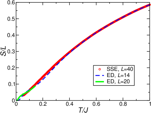
We test and compare the aforementioned numerical methods using the example of the $s=1$ Heisenberg chain (1) with a finite magnetization. Fig. 1 shows the entropy per site $S/L$ as a function of temperature $T$ for a fixed magnetic field $h=3\,J$. For $L=14$, we have performed a full diagonalization. The corresponding ED curve can therefore be considered as the exact result for $L=14$.

A full determination of the spectrum is clearly out of reach already for $L=20$. In this case, we therefore had to perform a severe truncation to low energies. Thus, the $L=20$ ED curve is only a low-temperature approximation. In this paper, the precise temperature range is fixed as follows: Let ${\cal E}$ be the highest energy until which the spectrum is definitely complete. Then we restrict to temperatures $T\leq{\cal E}/5$. This choice ensures that missing states are suppressed by a Boltzmann factor $\leq\exp(-5)\approx 0.006738$. This may seem a small number, but since we are discarding many states, extending truncated data to higher temperatures would yield artifacts which are clearly visible on the figure(s).

QMC (denoted by SSE in Fig. 1) is able to treat the larger system size $L=40$. This method, however, is best suited for high temperatures. Indeed, at $T\approx 0.05\,J$ one can see deviations caused by statistical errors in the SSE result of Fig. 1 which prevented us from going to lower temperatures. Finite-size effects can be observed in Fig. 1 in the $L=14$ ED curve for $T\lesssim 0.4\,J$ and in the $L=20$ ED result. Otherwise it is reassuring that we observe good overall agreement between all three methods.

In passing we note that, for the value of the magnetic field used in Fig. 1, the low-energy physics of the $s=1$ chain is described by a Luttinger liquid (see Ref. [47] and references therein). It is well known that the specific heat $C$ of a Luttinger liquid is linear in $T$ [48]. Due to the relation $C=T\,(\partial\,S/\partial T)$ and because of $S(T=0)=0$, the entropy of a Luttinger liquid is identical to its specific heat and in particular also linear in $T$. Indeed, Fig. 1 is consistent with a linear behavior $S\propto T$ at sufficiently large $L$ and low $T$.

3 Spin $s=1$ Heisenberg chain

Figure 2: Isentropes, i.e., adiabatic demagnetization curves of the $s=1$ Heisenberg chain as obtained from ED and QMC for different chain lengths. The corresponding values of the entropy are $S/L=0.05$, $0.1$, $0.15$, $0.2$, $0.25$, $\ldots$ (bottom to top).

In this section we will discuss the entropy of the $s=1$ Heisenberg chain in more detail.

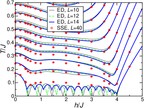
First, we show results for the value of the entropy per site $S/L$ as a function of $h$ and $T$ in Fig. 2. The ED curves have been obtained by computing the entropy $S$ on a mesh in the $h$-$T$-plane and determining the constant entropy curves, i.e., the isentropes from this data. This leads to some discretization artifacts at the cusps in the the $S/L=0.05$ curves (the ED curves at the lowest temperature) in Fig. 2. Conversely, the QMC had problems to resolve the large low-temperature entropy around the saturation field $h_{\rm sat.}=4\,J$. Accordingly, the $L=40$ SSE data points with $S/L=0.05$ are missing at $h/J=3.7$ and $4$. From our QMC simulations we can just conclude that for an $L=40$ chain these two points are in the region $T<0.067\,J$ and $T<0.085\,J$ for $h=3.7\,J$ and $4\,J$, respectively.

The ED curves with $S/L=0.05$ in Fig. 2 have marked finite-size wiggles. Also at higher temperatures (entropies), finite-size effects can be observed. There are, however, two regions where finite-size effects are evidently small. One is the low-temperature regime for fields $h$ smaller than the Haldane gap [29, 30]

$$\Delta\approx 0.4105\,J\,.$$ (11)

Also in the gapped high-field regime above the saturation field $h\gtrsim 4\,J$ one observes essentially no finite-size effects at any temperature. This renders ED the method of choice at high fields $h\gtrsim h_{\rm sat.}$, in particular at low temperatures, while QMC is preferable otherwise because bigger system sizes $L$ are accessible.

One can read off from Fig. 2 pronounced temperature changes in two regimes. Firstly, one can obtain cooling by adiabatic demagnetization from a high magnetic field $h>h_{\rm sat.}$ as one lowers the field to the saturation field. Secondly, at low temperatures, one can also cool by adiabatic magnetization from $h=0$ to $h=\Delta$. This demonstrates that one can use the gap-closing at a generic field-induced quantum phase transition for cooling purposes. In the regime $0.4105\,J\approx\Delta<h<h_{\rm sat.}=4\,J$, the spectrum is gapless (compare Fig. 1 and the related discussion in section 2.3). Accordingly, one observes only small temperature changes induced by adiabatic (de)magnetization in this field range.

Figure 3: Entropy per spin of the $s=1$ Heisenberg chain at zero magnetic field $h=0$ as a function of temperature. Note that the temperature axis is scaled as $1/T$ and the entropy axis logarithmically. The dashed line is a fit to (12) with ${\cal A}=0.577$ and $\Delta=0.4105\,J$.

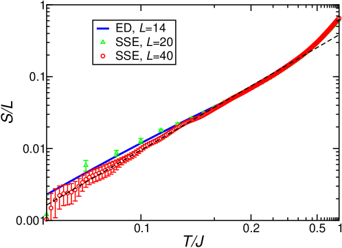
We now focus on the low-field regime. Firstly, we consider the behavior of the entropy at $h=0$ which is shown in Fig. 3. One observes that finite-size effects are small for $L\geq 14$: the $L=14$ curve is almost within the error margins of the $L=40$ QMC curve even at low temperatures. This can be attributed to a finite correlation length $\xi$ which is evidently sufficiently smaller than $14$ for all temperatures at $h=0$. Indeed, the correlation length of the $s=1$ Heisenberg chain is known to be $\xi\approx 6$ at $h=0$ and $T=0$ [29, 30].

Because of the presence of a gap $\Delta$ at $h=0$, we expect the entropy to be exponentially activated as a function of temperature. Accordingly, the low-temperature asymptotic behavior at $h=0$ should follow the form

$$\left.\frac{S}{L}\right|_{h=0}={\cal A}\,{\rm e}^{-\Delta/T}\,.$$ (12)

If we fix the gap to the known value $\Delta=0.4105\,J$ [29, 30], the only free parameter in the low-temperature asymptotic behavior (12) is the prefactor ${\cal A}$. A fit of the $L=40$ QMC results yields ${\cal A}=0.577(1)$. The dashed line in Fig. 3 shows that the formula (12) describes the low-temperature regime quite well with the given parameters.

Figure 4: Entropy per spin of the $s=1$ Heisenberg chain at $h=0.4105\,J$, corresponding to the Haldane gap. Note the doubly logarithmic scale. The dashed line shows the square-root behavior (13) with ${\cal B}=0.1323$.

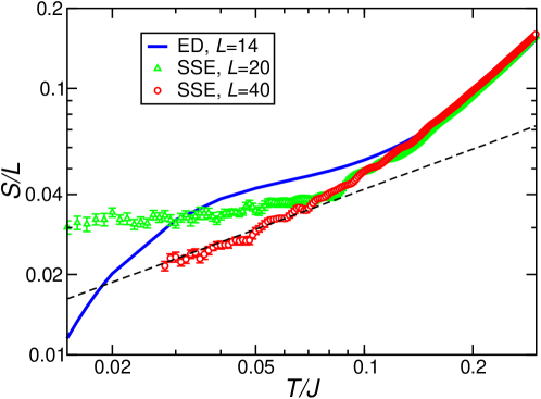
Secondly, we consider a magnetic field exactly equal to the Haldane gap $h=0.4105\,J$. Fig. 4 shows a doubly-logarithmic plot of the entropy $S$ as a function of temperature $T$ for this value of the magnetic field. Since we are now sitting at a field-induced quantum phase transition, we expect a large number of low-lying states and relatedly an infinite correlation length $\xi=\infty$. On a finite system, these low-lying states will be pushed to higher energies. Indeed, we observe pronounced finite-size effects at low temperatures in Fig. 4.

At a quantum phase transition in one dimension which preserves a $U(1)$-symmetry, the entropy $S$ is expected [4, 10, 6, 7] to vary asymptotically as a square root of temperature:

$$\left.\frac{S}{L}\right|_{h=\Delta}={\cal B}\,\sqrt{\frac{T}{J}}\,.$$ (13)

As before, the amplitude ${\cal B}$ is the only free parameter. A fit to the $L=40$ QMC data with $T\leq 0.07\,J$ yields ${\cal B}=0.1323(6)$. The dashed line in Fig. 4 shows that the $L=40$ QMC data is indeed consistent with the asymptotic square root (13) in the range $0.03\lesssim T/J\lesssim 0.07$. However, because of finite-size effects, in this case we really need to go to $L=40$ to recover the asymptotic behavior. Furthermore, we need to restrict to $T\lesssim 0.07\,J$ since one can see from Fig. 4 that a pure power law is no longer a good description for $T\gtrsim 0.07\,J$.

Comparison of (12) and (13) shows that one can reach exponentially small temperatures $T_{\rm f}$ at $h=\Delta$ by adiabatic magnetization of a spin-$1$ Heisenberg chain from an initial temperature $T_{\rm i}$ at $h=0$. For an initial temperature $T_{\rm i}\lesssim 0.1\,J$, the final temperature $T_{\rm f}$ can be quantitatively estimated from the following combination of (12) and (13)

$$\frac{T_{\rm f}}{J}=\frac{{\cal A}^{2}}{{\cal B}^{2}}\,{\rm e}^{-2\,\Delta/T_{\rm i}}\,,$$ (14)

with the parameters $\Delta$, ${\cal A}$, and ${\cal B}$ given above.

4 Scaling with spin quantum number $s$

We will now turn to the high-field region and consider in particular scaling with the spin quantum number $s$ close to the saturation field.

Figure 5: Isentropes of $L=20$ Heisenberg chains as obtained by ED for different $s$. Note that a truncation of the energy spectrum has been used for $s>1/2$. The values of the entropy per site are $S/L=0.05$, $0.01$, $0.15$, $0.2$, and $0.25$ (bottom to top).

It is straightforward to compute the excitation energy $\varepsilon$ of a single flipped spin propagating above a ferromagnetically polarized background (see, e.g., [49]):

$$\varepsilon(k)=2\,J\,s\,\left(\cos k-1\right)+h\,.$$ (15)

The minimum of this one-magnon dispersion is located at $k=\pi$. The saturation field $h_{\rm sat.}$ of the spin-$s$ Heisenberg chain (1) is given by the one-magnon instability [50]. Accordingly, it can be determined by inserting the condition $\varepsilon(\pi)=0$ into (15):

$$h_{\rm sat.}=4\,J\,s\,.$$ (16)

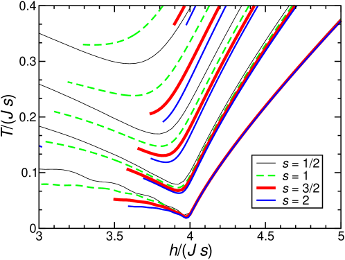
The fact that the single-particle energy (15) scales linearly with $s$ suggests to scale all energies close to the saturation field and at low temperatures linearly with $s$. In order to test this scenario, we have first computed the isentropes for a fixed chain length $L=20$ and $s\leq 2$. The $s=1/2$ curves are obtained by a full diagonalization of the Hamiltonian [10] while we have performed additional ED computations for $s=1$, $3/2$, and $2$ using the truncation procedure described in section 2. Fig. 5 shows the resulting isentropes for $S/L=0.05$, $0.01$, $0.15$, $0.2$, and $0.25$ close to the saturation field (16). We observe that at low temperatures, scaling both $h$ and $T$ by $s$ leads to a nice collapse of the isentropes around and in particular above the saturation field.

Figure 6: Specific heat per site $C/L$ (left column) and magnetic susceptibility per site $\chi/L$ (right column) as obtained by ED for different $s$. Note that a truncation of the energy spectrum has been used for $s>1/2$. The values of the magnetic field are chosen somewhat above the saturation field (top row), exactly at the the saturation field (middle row), and somewhat below the saturation field (bottom row).

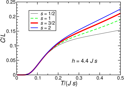
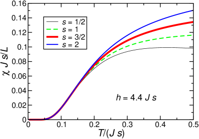
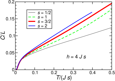
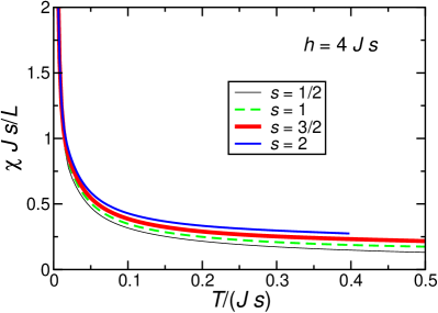
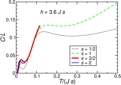
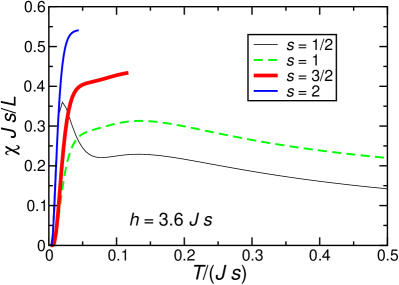
Further details can be read off from the temperature scans at a fixed magnetic field shown in Fig. 6. In this figure, we have chosen to show the specific heat $C$ as a representative for energy-related quantities and the magnetic susceptibility $\chi$ as a representative for magnetic quantities. The top row of Fig. 6 corresponds to a magnetic field $h=1.1\,h_{\rm sat.}$. Here we observe a nice collapse with $s$ for $T/(J\,s)\lesssim 0.15$. The middle row of Fig. 6 corresponds to a magnetic field exactly equal to the saturation field. Here we observe a good scaling collapse for $T/(J\,s)\lesssim 0.04$. Finally, the bottom row of Fig. 6 corresponds to a magnetic field $h=0.9\,h_{\rm sat.}$. In this case, one expects the scaling region to be pushed to even lower temperatures. However, for $h<h_{\rm sat.}$ the finite size $L=20$ leads to artifacts in the low-temperature behavior. Therefore it is difficult to make definite statements for this case.

To summarize this section, we have provided evidence of linear scaling with $s$ for thermodynamic quantities of spin-$s$ Heisenberg chains close to the saturation field. Note that this is very different from the quadratic scaling, e.g. of $T$ with $s^{2}$ [23] or with $s\,(s+1)$ [51, 52], which is needed to approach the classical limit.

5 Conclusions and outlook

In this paper we have illustrated the numerical computation of thermodynamic quantities and in particular the entropy for spin-$s$ Heisenberg chains. From a technical point of view, we have described in section 2.1 how to perform a reliable computation of a large number of low-lying states using the Lanczos method and in section 2.2 how to compute the entropy directly by a QMC simulation.

In section 3 we have then focused on the $s=1$ Heisenberg chain and shown in particular that one can cool with an adiabatic magnetization process during which the Haldane gap $\Delta$ is closed. Many previous investigations (e.g., [9, 10, 14, 18, 19, 23]) have focused on the saturation field. The reason for this is that the saturation field is a field-induced quantum phase transition at a known value of the magnetic field which also gives rise to technical simplifications. However, the scenario of quantum phase transitions [6, 7] is universal and not restricted to the saturation field. Indeed, Fig. 4 is consistent with the same universal square-root behavior of the entropy $S$ at $h=\Delta$ in the spin-1 Heisenberg chain as observed previously for $s=1/2$ chains exactly at the saturation field [4, 10]. This may also be important from an experimental point of view since a possible spin gap may be accessible by laboratory magnetic fields even if the saturation field is out of reach. In fact, cooling by adiabatic magnetization when closing a spin gap has presumably been indirectly observed in pulse-field magnetization experiments on SrCu₂(BO₃)₂ [53].

In section 4 we then moved to the saturation field and investigated scaling with the spin quantum number $s$. In contradistinction to the classical scaling regime where temperature should scale quadratically with $s$ [23, 51, 52], there is a quantum scaling regime around the saturation field where one observes a collapse using the linearly scaled parameters $h/s$ and $T/s$. Also in higher dimensions the one-magnon dispersion typically scales with $s$. By the same arguments as in section 4, we therefore expect linear scaling with $s$ at any continuous transition to saturation. This expectation could be tested numerically with the methods of the present paper.

References

- 1. Warburg E., Ann. Phys. Chem., 1881, 13, 141.
- 2. Giauque W.F., MacDougall D.P., Phys. Rev., 1933, 43, 768.
- 3. Bonner J.C., Fisher M.E., Proc. Phys. Soc., 1962, 80, 508.
- 4. Bonner J.C., Nagle J.F., Phys. Rev. A, 1972, 5, 2293.
- 5. Bonner J.C., Johnson J.D., Physica, 1977, 86-88B, 653.
- 6. Zhu L., Garst M., Rosch A., Si Q., Phys. Rev. Lett., 2003, 91, 066404.
- 7. Garst M., Rosch A., Phys. Rev. B, 2005, 72, 205129.
- 8. Tachiki M., Yamada T., J. Phys. Soc. Jpn., 1970, 28, 1413.
- 9. Zhitomirsky M.E., Phys. Rev. B, 2003, 67, 104421.
- 10. Zhitomirsky M.E., Honecker A., J. Stat. Mech.: Theor. Exp., 2004, P07012.
- 11. Zhitomirsky M.E., Tsunetsugu H., Phys. Rev. B, 2004, 70, 100403.
- 12. Derzhko O., Richter J., Phys. Rev. B, 2004, 70, 104415.
- 13. Sosin S.S., Prozorova L.A., Smirnov A.I., Golov A.I., Berkutov I.B., Petrenko O.A., Balakrishnan G., Zhitomirsky M.E., Phys. Rev. B, 2005, 71, 094413.
- 14. Honecker A., Wessel S., Physica B, 2006, 378-380, 1098.
- 15. Derzhko O., Richter J., Eur. Phys. J. B, 2006, 52, 23.
- 16. Čanová L., Strečka J., Jaščur M., J. Phys.: Condens. Matter, 2006, 18, 4967.
- 17. Gencer H., Int. J. Mod. Phys. B, 2006, 20, 2527.
- 18. Schmidt B., Shannon N., Thalmeier P., J. Phys.: Conf. Ser., 2006, 51, 207.
- 19. Schmidt B., Thalmeier P., Shannon N., Phys. Rev. B, 2007, 76, 125113.
- 20. Schnack J., Schmidt R., Richter J., Phys. Rev. B, 2007, 76, 054413.
- 21. Radu T., Tokiwa Y., Coldea R., Gegenwart P., Tylczynski, Z., Steglich F., Sci. Technol. Adv. Mater., 2007, 8, 406.
- 22. Pereira M.S.S., de Moura F.A.B.F., Lyra M.L., Phys. Rev. B, 2009, 79, 054427.
- 23. Honecker A., Zhitomirsky M.E., J. Phys.: Conf. Ser., 2009, 145, 012082.
- 24. Boyarchenkov A.S., Bostrem I.G., Ovchinnikov A.S., Phys. Rev. B, 2007, 76, 224410.
- 25. Tsui Y., Wolf B., Jaiswal-Nagar D., Tutsch U., Honecker A., Remović-Langer K., Prokofiev A., Assmus W., Donath G., Lang M., in preparation.
- 26. Klümper A., Honecker A., Ohanyan V., Trippe C., in preparation.
- 27. Haldane F.D.M., Phys. Rev. Lett., 1983, 50, 1153.
- 28. Haldane F.D.M., Phys. Lett. A, 1983, 93, 464.
- 29. White S.R, Huse D.A., Phys. Rev. B, 1993, 48, 3844.
- 30. Golinelli O., Jolicoeur Th., Lacaze R., Phys. Rev. B, 1994, 50, 3037.
- 31. Bonner J.C., Fisher M.E., Phys. Rev., 1964, 135, A640.
- 32. Bonner J.C., Numerical Studies on the Linear Ising-Heisenberg chain. PhD thesis, University of London, 1968.
- 33. Greenbaum A., Dongarra J., Experiments with QR/QL Methods for the Symmetric Tridiagonal Eigenproblem. LAPACK working note 17, 1989.
- 34. Honecker A., Schüle J., OpenMP Implementation of the Householder Reduction for Large Complex Hermitian Eigenvalue Problems. – In: Advances in Parallel Computing 15, Lippert T., Mohr B., Peters F. (Eds.), IOS Press, 2008,
- 35. Lanczos C., J. Res. Nat. Bur. Standards, 1950, 45, 255.
- 36. Cullum J.K., Willoughby, R.A., Lanczos Algorithms for Large Symmetric Eigenvalue Computations. Vol. I: Theory. SIAM Classics in Applied Mathematics 41, 2002.
- 37. Bai Z., Demmel J., Dongarra J., Ruhe A., van der Vorst H., Templates for the Solution of the Algebraic Eigenvalue Problems. A Practical Guide. SIAM, Philadelphia, 2000.
- 38. Troyer M., Wessel S., Alet F., Phys. Rev. Lett., 2003, 90, 120201.
- 39. Troyer M., Alet F., Wessel S., Braz. J. of Phys., 2004, 34, 377.
- 40. Wessel S., Stoop N., Gull E., Trebst S., Troyer M., J. Stat. Mech., 2007, P12005.
- 41. Sandvik A.W., Kurkijärvi J., Phys. Rev. B, 1991 43, 7.
- 42. Sandvik A.W., Phys. Rev. B, 1999, 59, R14157.
- 43. Syljuåsen O.F., Sandvik A.W., Phys. Rev. E, 2002, 66, 046701.
- 44. Alet F., Wessel S., Troyer M., Phys. Rev. E, 2005, 71, 036706.
- 45. Wang F., Landau D.P., Phys. Rev. Lett., 2001, 86, 2050.
- 46. Wang F., Landau D.P., Phys. Rev. E, 2001, 64, 056101.
- 47. Fáth G., Phys. Rev. B, 2003, 68, 134445.
- 48. Giamarchi T., Quantum Physics in One Dimension. Clarendon Press, Oxford, 2004.
- 49. Hodgson R.P., Parkinson J.B., J. Phys. C: Solid State Phys., 1985, 18, 6385.
- 50. Parkinson J.B., Bonner J.C., Phys. Rev. B, 1985, 32, 4703.
- 51. Kim Y.J., Greven M., Wiese U.J., Birgeneau R.J., Eur. Phys. J. B, 1998, 4, 291.
- 52. Engelhardt L., Luban M., Schröder C., Phys. Rev. B, 2006, 74, 054413.
- 53. Levy F., Sheikin I., Berthier C., Horvatić M., Takigawa M., Kageyama H., Waki T., Ueda Y., Europhys. Lett., 2008, 81, 67004.
- 54. Alet F. et al., J. Phys. Soc. Jpn. Suppl., 2005, 74, 30.
- 55. Albuquerque A.F. et al., J. Magn. Magn. Mater., 2007, 310, 1187.