Out of equilibrium dynamics of the spiral model

Abstract

We study the relaxation of the bi-dimensional kinetically constrained spiral model. We show that due to the reversibility of the dynamic rules any unblocked state fully decorrelates in finite times irrespectively of the system being in the unjammed or the jammed phase. In consequence, the evolution of any unblocked configuration occurs in a different sector of phase space from the one that includes the equilibrium blocked equilibrium configurations at criticality and in the jammed phase. We argue that such out of equilibrium dynamics share many points in common with coarsening in the one-dimensional Ising model and we identify the coarsening structures that are, basically, lines of vacancies. We provide evidence for this claim by analyzing the behaviour of several observables including the density of particles and vacancies, the spatial correlation function, the time-dependent persistence and the linear response.

PACS: 05.70.Ln, 75.40.Gb, 05.40.-a

I Introduction

Kinetically constrained models are toy models for the glassy phenomenon FA  (see Jackle ; Sollich ; Leonard for reviews). These models display no thermodynamic singularity: their equilibrium measure is simply the Boltzmann factor of independent variables and correlations only reflect the hard core constraint. Still, they capture many features of real glass-forming systems; among them one can mention stretched exponential relaxation FB , super-Arrhenius equilibration time GPG , dynamical heterogeneity KA and self-diffusion/viscosity decoupling H . They also display glassy out of equilibrium aspects, such as physical aging KPS and effective temperatures S (for a review of these aspects see Leonard ) that are similar to the ones first obtained in random $p$-spin systems Cuku ; Cukupe , as well as heterogeneous aging relaxation Chamon . Bootstrap percolation arguments allowed C. Toninelli et al. to show that most finite dimensional kinetically constrained models studied so far do not even have a dynamic transition at a particle density that is less than unity in the thermodynamic limit Cristina0 . On Bethe lattices instead a dynamical transition similar to the one predicted by the mode coupling theory might occur Sellitto .

A finite dimensional kinetically constrained model with an ideal glass-jamming dynamic transition at a particle density that is different from one, the two-dimensional spiral model, was introduced in a series of papers by C. Toninelli et al. Cristina ; Cristina1 ; Cristina2 ; Cristina3 . The dynamic transition is defined as the critical density at which an equilibrium configuration can no longer be emptied by applying the dynamic rule. In consequence, at the transition an infinite cluster of particles (or spins in an equivalent representation) that are blocked by the dynamic constraints exists. The model is defined on a square lattice and the transition occurs at a value of the control parameter $p$, the probability to update an unblocked site, that coincides with the critical threshold of directed site percolation in $d=2$, that is to say, $p_{c}\simeq 0.705$. The density of the frozen cluster is discontinuous at $p_{c}$ which means that the frozen structure is compact rather than fractal at criticality. Thus, at and above $p_{c}$ a finite fraction of particles are blocked. It was shown in these papers that approaching the critical $p_{c}$ from the unjammed phase the decorrelation of an equilibrium configuration decays in two steps similarly to what is common in glass-forming liquids. The time-scale for relaxation – say the $\alpha$ relaxation time – diverges with a Vogel-Fulcher law (faster than a power law). A crossover length below which finite size effects are important also diverges faster than a power law when $p_{c}$ is approached from below.

In this paper we study the dynamics of the $2d$ spiral model numerically. For concreteness, we first show results for the equilibrium dynamics, meaning the relaxation of an equilibrium configuration, below but close to the critical $p_{c}$ – the ‘super-cooled liquid’ – and above $p_{c}$ – the ‘equilibrium glass’. Next, we focus on the out of equilibrium kinetics. Specifically, we consider annealing and quenching processes. In the former the system is prepared in an equilibrium initial condition at $p_{0}\geq p_{c}$ and subsequently brought into the glassy regime with $p>p_{0}$ by using a finite rate of change of the parameter $p$. In the latter we study the evolution after a sudden quench, in which an equilibrium state at $p_{0}=0$ (completely empty configuration) is evolved from time $t=0$ onwards with the dynamic rule specified by a different value of $p>p_{0}$. This procedure is similar to the temperature quench of a liquid. For $p<p_{c}$, after a non equilibrium transient the system attains the unblocked equilibrium state. The relaxation time for attaining such a state diverges as $p\to p_{c}$. In the critical case with $p=p_{c}$, the system approaches the blocked equilibrium state by means of an aging coarsening dynamics with some points in common with the ones observed in critical quenches of ferromagnetic models. Freezing is not observed because the dynamic density $\rho(t)$ is always smaller than the critical one $\rho_{c}=p_{c}$, at any finite time. A different situation occurs for filling at $p>p_{c}$. Also in this case the system keeps evolving up to the longest observed times and a blocked state is never observed despite the fact that $\rho(t)$ exceeds $\rho_{c}$ for long enough times. This can be understood by noticing that the dynamics are fully reversible: for any $p$, each configuration reached dynamically can always evolve back to the initial state with $\rho<p_{c}$ by the time reversed process, although with a very low probability. Therefore, states with blocked regions cannot be dynamically connected to the initial unblocked states and they cannot be reached by any reversible process. Frozen regions being dynamically forbidden, the system approaches a high density ($\rho>\rho_{c}$) ensemble which does not contain any of the blocked states the measure of which is relevant in equilibrium. This feature recalls what happens in coarsening systems where, again for dynamical reasons, the kinetics occurs on the ensemble of configurations with vanishing magnetization the weight of which is negligible in equilibrium Palmer . Actually, it will be shown that the dynamics of the spiral model at $p>p_{c}$ strongly resembles coarsening in ferromagnets.

II Model

A binary variable $n_{ij}=0,1$ is defined on the sites $(i,j)$ of an ${\cal L}\times{\cal L}$ square lattice in $d=2$. $n_{ij}=1$ corresponds to a particle, $n_{ij}=0$ to a vacancy. For a given position $(i,j)$, let us define the following couple of neighbouring sites (see Fig. 1)

• $(i,j+1)$,$(i+1,j+1)$, north east (NE) couple

• $(i+1,j)$,$(i+1,j-1)$, south east (ES) couple

• $(i,j-1)$,$(i-1,j-1)$, south west (SW) couple

• $(i-1,j)$,$(i-1,j+1)$, north east (WN) couple

Figure 1: (Color online.) The neighbouring sites determining the frozen or free to move character of the center site $(i,j)$.

The possibility to update the variable $n_{ij}$ depends on the configuration of such couples. Specifically, if the sites belonging to at least two consecutive couples (namely, NE+SE or SE+SW or SW+NW or NW+NE) are empty (otherwise stated occupied by vacancies), then site $(i,j)$ can be updated (either emptied or filled). Otherwise it is blocked. We consider each site coupled to a particle reservoir in such a way that particles can enter or leave the sample from its full volume, in contrast to what was used in KPS , for instance, where particles were allowed to access or leave the ($3d$ in this case) system only through the borders. We use periodic boundary conditions.

Defining the variable $M_{ij}$ such that $M_{ij}=0$ if site $(i,j)$ is frozen, and $M_{ij}=1$ otherwise the updating rule can be compactly expressed in terms of the transition rates $W_{p}(n_{ij}|n^{\prime}_{ij})$ to go from $n$ to $n^{\prime}$ on site $(i,j)$ as

$$W_{p}(0|1)=M_{ij}\ p\qquad\qquad W_{p}(1|0)=M_{ij}\ (1-p).$$ (1)

The equilibrium state has been studied in detail by C. Toninelli et al. Cristina ; Cristina1 . The model can be regarded as a two-level system described by the Hamiltonian $H[s]=-\sum_{ij}n_{ij}$ at the inverse temperature

$$\beta=\ln[p/(1-p)]\;.$$ (2)

When $p\to 1/2$ the inverse temperature vanishes $\beta\to 0$ whereas for $p\to 1$ it diverges $\beta\to\infty$. The Bernoulli measure implies $\rho=\langle n_{ij}\rangle=p$ for the equilibrium density of particles. This means that, in equilibrium at zero temperature ($p\to 1$), the lattice is full while at infinite temperature ($p\to 1/2$) it is half-filled. The existence of a blocked cluster at $p\geq p_{c}<1$ was shown by studying the critical $p$ above which an equilibrium configuration cannot be emptied.

Figure 2: (Colour online.) Equilibrium configurations at (a) $p=0.5<p_{c}$ , (b) $p_{c}\simeq 0.705$, and (c) $p=0.99>p_{c}$. The colour code is such that: a filled blocked site is black; an empty blocked site is white; a free particle (one that can be removed) is red and a free vacancy (one that can be filled) is green. We show a small fraction of the sample to make the snapshot easier to visualize.

Interestingly enough the microscopic dynamic rules are fully reversible. This implies that an initial configuration with no blocked structure can never reach, via the dynamics, a state with a blocked sub-ensemble of sites within. This fact holds for a system coupled to the reservoir in any possible way (volume, border, or other). We shall elaborate on the consequences of this fact later in the paper.

III Observables

The dynamics of kinetically constraint models are usually studied in terms of the probability that a spin never flips between time $t_{w}$ and a later time $t$, also called the persistence function $\phi(t,t_{w})$. Operatively, we define this quantity as

$$\phi(t,t_{w})=\frac{1}{N}\langle N_{noup}(t,t_{w})\rangle,$$ (3)

where $N={\cal L}\times{\cal L}$ is the number of lattice points, $N_{noup}(t,t_{w})$ is the number of sites that have not been updated between $t_{w}$ and $t$ in a given realization of the dynamics and $\langle\dots\rangle$ denotes an average over different histories and initial conditions. In equilibrium conditions one has $\phi(t,t_{w})=\phi(t-t_{w})$. Moreover, at and above $p_{c}$ one has $\phi_{\infty}\equiv\lim_{t\to\infty}\phi(t,t_{w})>0$ due to the frozen backbone, while below $p_{c}$ the asymptotic value vanishes $\phi_{\infty}=0$.

Similar properties are exhibited by the autocorrelation function

$$C(t,t_{w})=\langle n_{ij}(t)n_{ij}(t_{w})\rangle-\langle n_{ij}(t)\rangle\langle n_{ij}(t_{w})\rangle.$$ (4)

The impulsive autoresponse function is defined as

$$R(t,t_{w})=\left.\frac{\delta\langle n_{ij}(t)\rangle}{\delta\epsilon_{ij}(t^{\prime})}\right|_{\epsilon_{ij}=0}$$ (5)

where $\epsilon_{ij}$ is a perturbation changing the transition rates as $W_{p}(n_{ij},n^{\prime}_{ij})\to W_{p+\epsilon_{ij}}(n_{ij},n^{\prime}_{ij})$. Notice that we dropped the site dependence in $C$ and $R$ due to space homogeneity. The integrated response function, or susceptibility, is

$$\chi(t,t_{w})=\int_{t_{w}}^{t}dt^{\prime}R(t,t^{\prime})\;.$$ (6)

In equilibrium conditions the response function is related to the autocorrelation function by the fluctuation-dissipation theorem (FDT)

$$T\chi(t,t_{w})=C(t,t)-C(t,t_{w})$$ (7)

where $T=\beta^{-1}$ with $\beta$ defined in Eq. (2) in the spiral model. Out of equilibrium the response function can still be related to correlation functions of the unperturbed system (with $\epsilon=0$) according to the generalization of the FDT derived in algo . This will allow us to determine the response function numerically without applying any perturbation.

It is useful to introduce the normalized autocorrelation function

$$\hat{C}(t,t_{w})=C(t,t_{w})/C(t,t)$$ (8)

and susceptibility

$$\hat{\chi}(t,t_{w})=\chi(t,t_{w})/C(t,t).$$ (9)

Finally, let us define

$$l(t)=[\rho_{eq}-\rho(t)]^{-1}.$$ (10)

In the non-equilibrium cases considered in Sec. V.2, when an initially empty state is progressively filled with the transition rates $W_{p}$ in Eq. (1), $\rho(t)$ always approaches $\rho_{eq}=p$. In this case $l(t)$ is a monotonically growing function of time, and it will be convenient to re-parametrize $t$ in terms of $l$.

The spatial evolution of the structure is usually monitored via the equal time correlation function (equivalently, in Fourier space, the structure factor):

$$G(r,t)=\langle n_{ij}(t)n_{i^{\prime}j^{\prime}}(t)\rangle-\langle n_{ij}(t)\rangle^{2}$$ (11)

where $r$ is the distance between sites $(i,j)$ and $(i^{\prime},j^{\prime})$. A typical length can be extracted from $G$ by using

$$L(t)=\left[\frac{\int dr\ r^{\alpha}\ G(r,t)}{\int dr\ G(r,t)}\right]^{1/\alpha}.$$ (12)

When scaling holds, namely $G(r,t)/G(0,t)=g(r/L(t))$, changing $\alpha$ leads to the same determination of $L(t)$ apart from a multiplicative constant.

All our simulations are done with square systems with linear size ${\cal L}=200-2000$, depending on the situation. We typically average over $10^{2}-10^{4}$ realizations of the dynamics.

IV Equilibrium relaxation

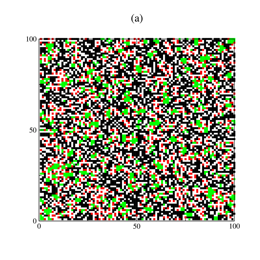
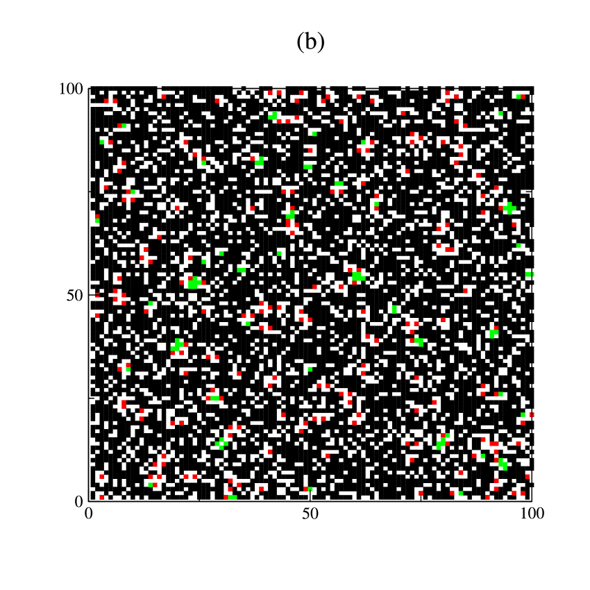
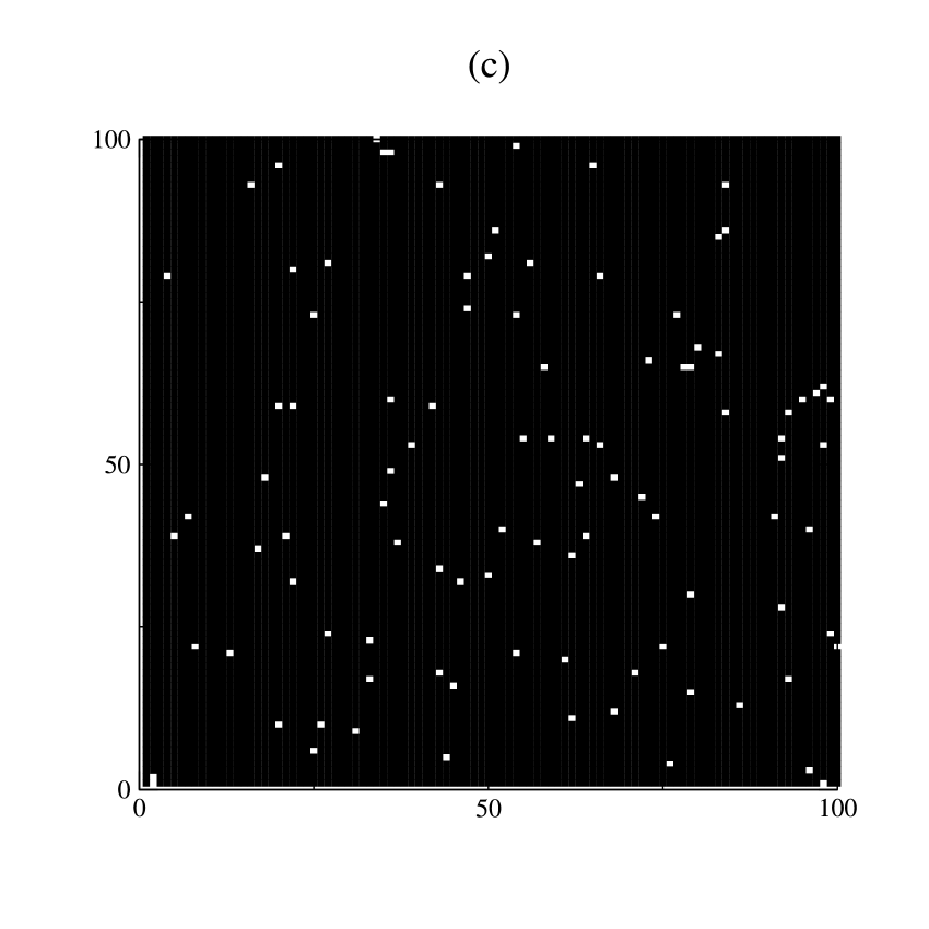
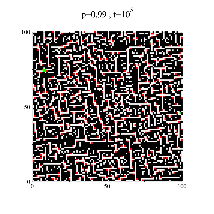
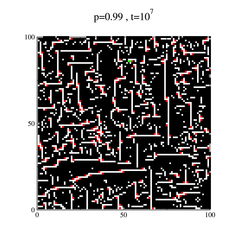
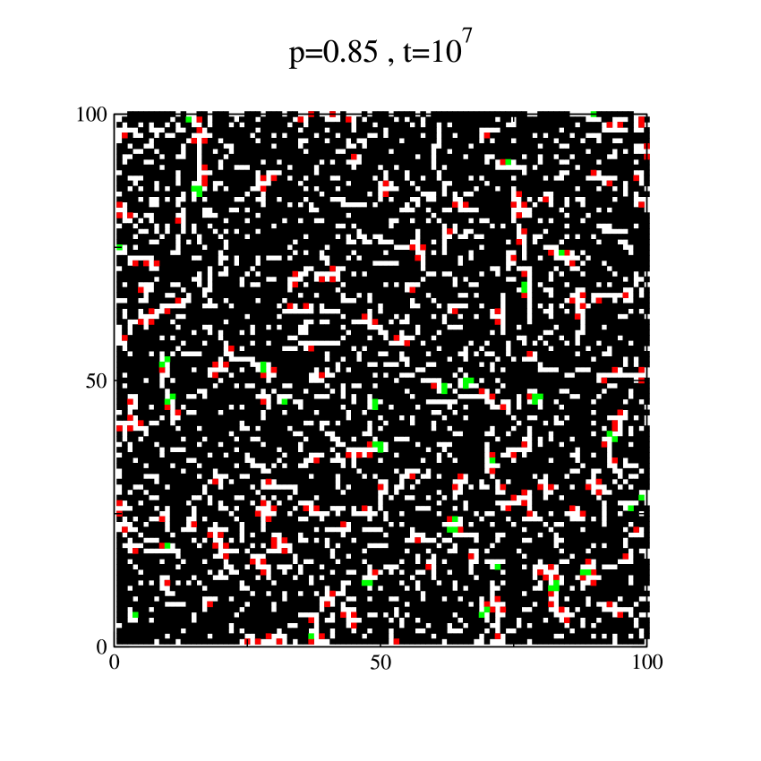
Figure 2 displays three panels with equilibrium configurations at $p<p_{c}$ (a), $p=p_{c}$ (b) and $p>p_{c}$ (c). We shall later confront these images to the ones reached dynamically from an empty state, see Fig. 8.

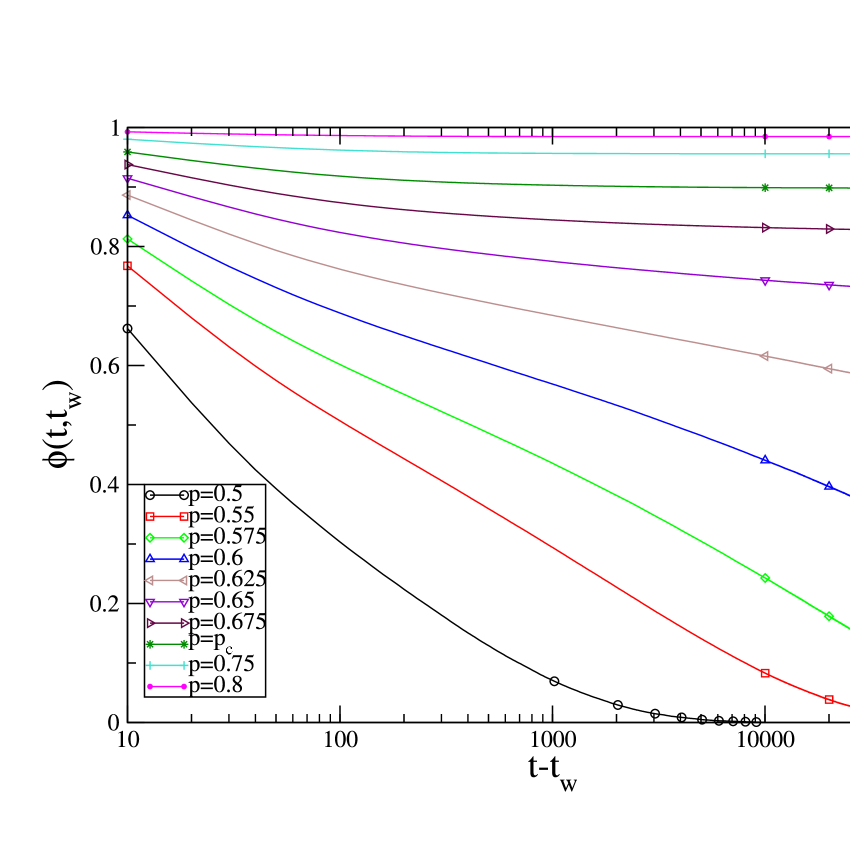
In Fig. 3(a) we study the relaxation of an equilibrium configuration for several values of $p$ by means of the persistence function. For values of $p<p_{c}$ there is no frozen structure in the system and the persistence function, $\phi$, decays to zero. Close to the critical $p_{c}$, although a blocked spanning structure does not exist, long living quasi-frozen structures do. The decay of the persistence or the normalized correlation close (but below) criticality is reminiscent of the hallmark of the super-cooled liquid relaxation that is associated to the formation of long-lived cages surrounding each particle Cavagna . The persistence of these structures diverges as $p_{c}$ is approached. As a consequence, $\phi(t,t_{w})$ develops a plateau that becomes longer and longer when $p$ gets closer to $p_{c}$ as in a super-cooled liquid. This numerical result confirms the analytic ones in Cristina ; Cristina1 ; Cristina2 ; Cristina3 .

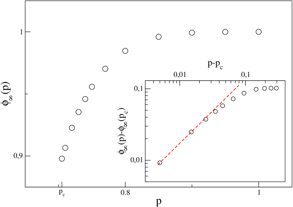
Above $p_{c}$ the initial configurations have a finite fraction of frozen particles so $\phi$ decays to a constant, $\phi_{\infty}$, that depends on $p$. Figure 3(b) shows $\phi_{\infty}(p)$. As expected $\phi_{\infty}$ is different from zero at $p_{c}$; we found $\phi_{\infty}(p_{c})\simeq 0.9$, a relatively large value. A fit to the data close to the critical point yields $\phi_{\infty}(p)\simeq\phi_{\infty}(p_{c})+c(p-p_{c})^{\alpha}$ with $\alpha\simeq 0.9$. $\phi_{\infty}$ increases with $p$ and reaches $1$ at $p\to 1$.

The normalized autocorrelation function $\hat{C}(t,t_{w})$ behaves in a qualitatively similar way. Moreover, consistently with equilibrium dynamics $\hat{C}(t,t_{w})$ is related to $\hat{\chi}(t,t_{w})$ by the FDT, namely $T\hat{\chi}(t,t_{w})=1-\hat{C}(t,t_{w})$, see Eq. (7).

Figure 3: (Color online.) Upper panel: Decay of the persistence function for an initial condition in equilibrium at different values of $p$. $\phi_{\infty}\equiv\lim_{t\to\infty}\phi(t)=0$ below $p_{c}$ and $\lim_{t\to\infty}\phi(t)>0$ above $p_{c}$. Lower panel: Dependence of $\phi_{\infty}$ on $p$. In the inset $\phi_{\infty}(p)-\phi_{\infty}(p_{c})$ is plotted against $p-p_{c}$ in a double logarithmic scale, for $p>p_{c}$. The red dashed line is the best fit to the power-law behavior $\phi_{\infty}(p)-\phi_{\infty}(p_{c})\propto(p-p_{c})^{\alpha}$, yielding $\alpha=0.901$.

V Out of equilibrium relaxation

In this Section we discuss the out of equilibrium dynamics of a system initially prepared in some equilibrium configuration at $p_{0}$ and then evolved from time $t=0$ onward with the transition rates (1) and $p>p_{0}$. As discussed in Sec. II this procedure is the analogue of a cooling experiment in thermal systems.

We shall consider two types of ‘cooling’ procedures: the former is a slow process where a system at equilibrium at $p=p_{0}\geq p_{c}$, a configuration with a blocked structure, is evolved with the transition rates (1) and a time-dependent $p=p_{0}+rt$, $r$ being the equivalent of a cooling rate. The latter is an instantaneous quench where an equilibrium system at $p_{0}=0$, a completely empty state, is evolved using $p<p_{c}$, $p=p_{c}$ and $p>p_{c}$ as target values of the control parameter for the subsequent dynamics.

We recall that the dynamic rule is reversible and configurations with or without a blocked sub-ensemble of sites are mutually inaccessible even for finite systems, a fact that draws an important difference with usual stochastic models without dynamical constraints.

V.1 Slow cooling from equilibrium at $p_{c}$: threshold level

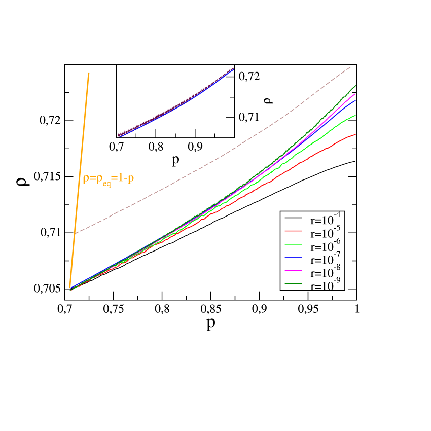
In Fig. 4 we show the density of particles found after cooling with a finite rate. Continuous lines with different colour represent processes starting from an equilibrium configuration at $p_{c}$ and using different cooling rates $r$. Dashed curves, instead, refer to cases where cooling starts from equilibrium above $p_{c}$. Concerning cooling from equilibrium at $p_{c}$, for $p$’s that are above but not too far from $p_{c}$ the curves for $r<10^{-7}$, say, superpose. For larger values of $p$ there is a residual $r$ dependence that presumably disappears for even smaller $r$’s. We assume then that the dark green curve is quite close to the one for the limit of vanishing cooling rate $\rho_{th}(p)\equiv\lim_{r\to 0}\rho_{r}(p)$. $\rho_{th}(p)$ is definitely below the equilibrium density $\rho_{eq}$ for all $p>p_{c}$ and hits a limit $\rho_{th}(1)\gtrsim 0.723<1$ when $p\to 1$.

This analysis demonstrates that the blocked structure at $p_{c}$ involves vacancies that cannot be filled when increasing $p$ with the cooling procedure and the dynamic density remains well below the equilibrium one (shown with a continuous straight orange line in Fig. 4). A similar procedure in which $T$ is changed infinitely slowly, carried out in the $p$-spin model with $p\geq 3$ defines the threshold free-energy level Cuku that remains higher than the equilibrium free-energy in the full low temperature phase.

Cooling with a finite rate an initial condition equilibrated at a value $p_{0}(>p_{c})$ yields other levels of blocked states (low lying metastable TAP states in the $p\geq 3$-spin analogy). In Fig 4 we show with a dashed line one of such curves with $p_{0}=0.71$. A more careful analysis shown in the inset suggests that the curves for different $p_{0}$ do not cross in the full $p>p_{c}$ region, again in accordance with the $p$-spin scenario in which there is neither level crossing nor level merging when $T$ is lowered infinitesimally slowly.

Figure 4: (Color online.) The density of particles as a function of $p$ for linear cooling rate procedures $p(t)=p_{0}+rt$ starting from equilibrium at $p_{0}\geq p_{c}$. Continuous curves: $p_{0}=p_{c}\simeq 0.705$ and different cooling rates $r$ given in the key. The annealed densities at fixed $p$ increase with decreasing $r$ but they remain well below the equilibrium values, $\rho_{eq}=p$, shown with an orange straight line in the figure. Dashed line: the initial condition is equilibrium at $p_{0}=0.71>p_{c}$ and the cooling rate is $r=10^{-7}$. In the inset the continuous and the dashed line represent the curves obtained with $r=10^{-7}$ starting from $p_{0}=p_{c}$ (continuous line) or $p_{0}=0.7051>p_{c}$.

V.2 Infinitely rapid quench from equilibrium at $p_{0}=0$.

In this Section we consider the dynamical process whereby an empty configuration is filled with the transition rate (1), for different values of $p$. We have checked that starting from an equilibrium configuration corresponding to $0<p_{0}<p_{c}$ (i.e. not completely empty), does not change the evolution significatively. In the case of quenches to $p>p_{c}$ the effect of $p_{0}>0$ is to delay the asymptotic regime where, as we shall discuss below, scaling holds. This is due to the more blocked nature of the initial state. For this reason, the choiche $p_{0}=0$ is the most convenient to study the asymptotic properties, and we shall always make this choice in the following.

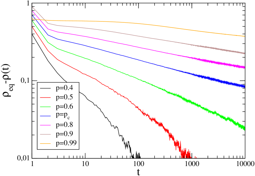
In Fig. 5 we plot the difference between $\rho_{eq}$ and the dynamic density $\rho(t)$. This quantity is related to $l(t)$ through Eq. (10). For $p<p_{c}$ the density decays exponentially to the equilibrium value over a typical time that increases as $p$ approaches $p_{c}$. At $p=p_{c}$, there is a power law decay $\rho(t)-\rho_{eq}\propto t^{-\nu(p_{c})}$ with $\nu(p_{c})\simeq 0.16$. For $p>p_{c}$, the same behavior, $\rho(t)-\rho_{eq}\propto t^{-\nu(p)}$ is observed, although the exponent $\nu(p)$ becomes smaller as $p$ increases and seems to go to zero in the limit $p\to 1$. Notice that this implies that $l(t)$ grows as a power law in the whole phase $p\geq p_{c}$, and logarithmically in the extreme limit $p\to 1$. The relaxation seems to be smooth in the sense that $\rho(t)$ decays as a power law within the whole explored time-window.

If one extrapolates the power law behaviour to infinitely long times the fact that $\rho_{eq}-\rho(t)\to 0$ would mean that, surprisingly enough, the relaxation avoids the threshold level – defined by the procedure described in Sect. V.1. Part of the explanation of this fact is that the dynamics are reversible and after a quench the system never reaches configurations with a completely blocked sub-ensemble. This implies that the system cannot go through threshold states to lower lying metastable ones since all the former do have blocked sub-ensembles. This is clearly different from what is the $p$-spin scenario in which a typical initial condition as the one corresponding to infinite temperature first relaxes to the threshold level Cuku ; Cavagna ; Montanari and then penetrates below it via thermal activation for finite size systems. It is also different from the behaviour of kinetically constrained spin models on the Bethe lattice Sellitto that seem to conform to the $p$-spin scenario. The fact that the out of equilibrium relaxation of the spiral model reaches $\rho(t)>\rho_{th}(p)$ implies that the dynamics should go to the long-time configurations ‘turning around’ blocked ones in phase space.

Figure 5: (Color online.) The difference between $\rho(t)$ and its equilibrium value $\rho_{eq}$ against time for different values of $p$. The relaxation is faster the smaller the value of $p$.

In the following Sections we shall discuss the three cases of quenches to $p<p_{c}$, $p=p_{c}$ and $p>p_{c}$ in more detail separately.

V.2.1 Quench from $p_{0}=0$ to $p<p_{c}$: equilibrium dynamics.

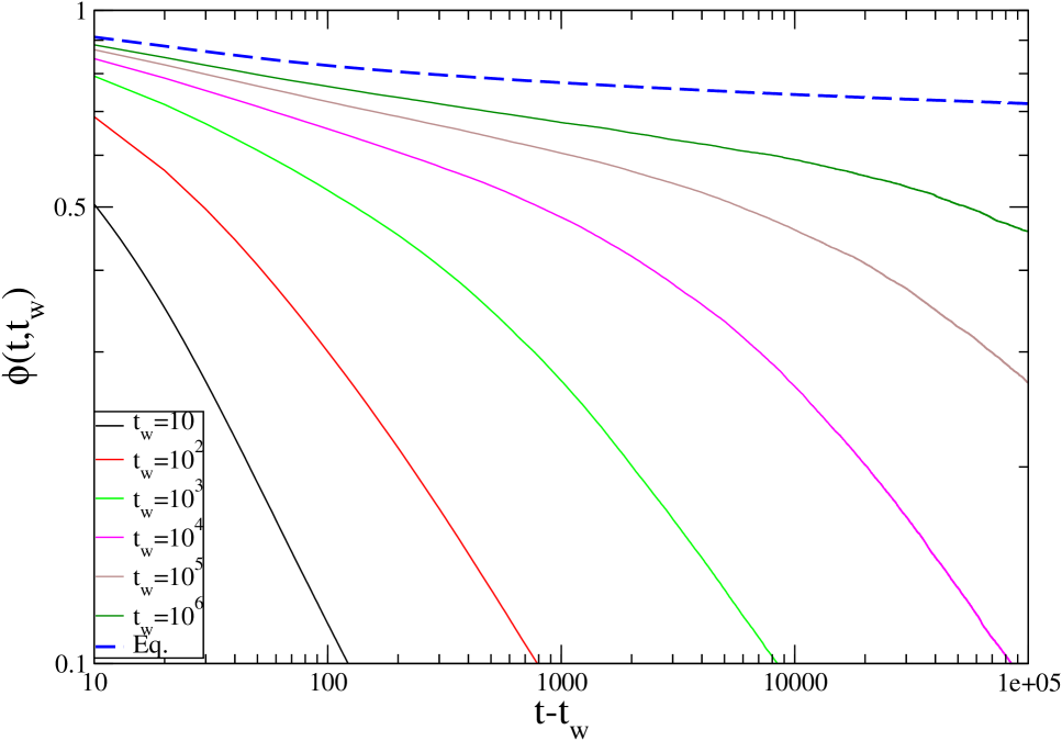
We have already observed that for $p<p_{c}$ but sufficiently close to $p_{c}$ long lasting quasi-blocked structures exist which are responsible for the development of a plateau in the persistence function. In the case considered here, since the initial configuration is empty, those structures must be built. Hence the plateau observed in equilibrium (Fig. 3) can be observed only in the limit $t_{w}\to\infty$, when equilibrium is attained and the long lived quasi-frozen structures are fully developed. For finite $t_{w}$, on the other hand, those structures are not completed and the plateau has a shorter extent, as shown in Fig. 6. $\hat{C}(t,t_{w})$ behaves similarly.

Figure 6: (Color online.) The persistence function $\phi(t,t_{w})$ is plotted against $t-t_{w}$ in the case of a quench from an empty configuration to $p=0.65$, for different values of $t_{w}$. The equilibrium curve (long dashed) is approached in the large-$t_{w}$ limit. The system is never blocked and $\phi$ decreases to zero in all cases.

V.2.2 Quench from $p=0$ to $p=p_{c}$: Critical quench.

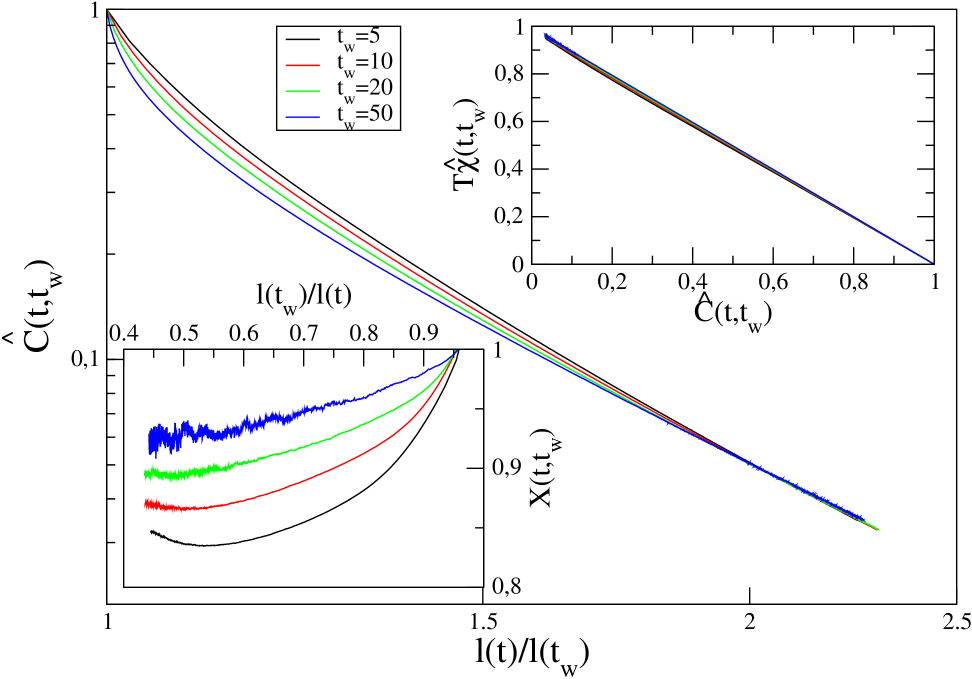
In this case a configuration with a blocked structure is approached in an infinite time but never reached. Since, as shown in Fig. 5, $\rho(t)$ approaches the equilibrium value asymptotically as a power law, we shall re-parametrize $t$ in terms of $l(t)$ in the following. We do this because, although $t$ and $l$ are trivially related in the asymptotic time domain, at early times when corrections to the power law behavior of $l$ are present, this quantity turns out to be better suited to enlighten the scaling properties of the dynamics. Since $\phi(t,t_{w})$ and $\hat{C}(t,t_{w})$ display the same scaling properties we discuss in the following the behavior of the latter quantity. The data of Fig. 7 show that $\hat{C}(t,t_{w})$ obeys the scaling

$$\hat{C}(t,t_{w})=f\left[\frac{l(t)}{l(t_{w})}\right].$$ (13)

The collapse of the curves for different $t_{w}$ is very good for large values of $x=l(t)/l(t_{w})\stackrel{{\scriptstyle>}}{{\sim}}1.75$, while it is poorer for smaller values of $x$ perhaps due to preasymptotic effects. The same scaling is found for the susceptibility, as testified by the fact that the parametric plot of $\hat{\chi}(t,t_{w})$ against $\hat{C}(t,t_{w})$ (upper inset of Fig. 7) does not depend on $t_{w}$. The parametric plot has the linear equilibrium behavior $T_{c}\hat{\chi}(t,t_{w})=1-\hat{C}(t,t_{w})$, as in ferromagnetic models quenched to $T_{c}$. However, while in the latter case the quantity $X(t,t_{w})=TR(t,t_{w})/(\partial C/\partial t_{w})$ is a non trivial function of $t/t_{w}$ with the limiting value $\lim_{t_{w}\to\infty}\lim_{t\to\infty}X(t,t_{w})=X_{\infty}<1$ xinfty , here $X(t,t_{w})$ slowly approaches $X(t,t_{w})\equiv 1$ in the limit $t_{w}\to\infty$, as shown in the lower inset of Fig. 7.

Figure 7: (Color online.) Dynamics after a quench from $p_{0}<p_{c}$ to $p_{c}$. $\hat{C}(t,t_{w})$ is plotted against $l(t)/l(t_{w})$. The upper inset shows the fluctuation-dissipation plot of $\hat{\chi}(t,t_{w})$ against $\hat{C}(t,t_{w})$. The lower inset shows the fluctuation-dissipation ratio $X(t,t_{w})$ as a function of $l(t_{w})/l(t)$.

V.2.3 Quench from $p_{0}=0$ to $p>p_{c}$: Coarsening.

We now discuss the dynamics following an infinitely rapid quench from equilibrium at $p_{0}=0$ to $p>p_{c}$. We argue that the relaxation occurs through a coarsening process which resembles some features of ferromagnetic systems. The kinetics simplifies in the limit $p\to 1$ because $W_{1}(1|0)/W_{1}(0|1)\to 0$ and the annihilation of particles can be neglected with respect to creation events if the latter are available. We shall consider this case first, since a cleaner description of the kinetics and of its basic mechanisms is possible. The case with a non-vanishing $1-p$ finite, where the finite annihilation probability adds new mechanisms to the kinetics, will be considered further below.

Quenches to $p\to 1$

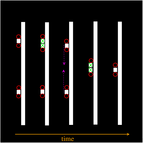
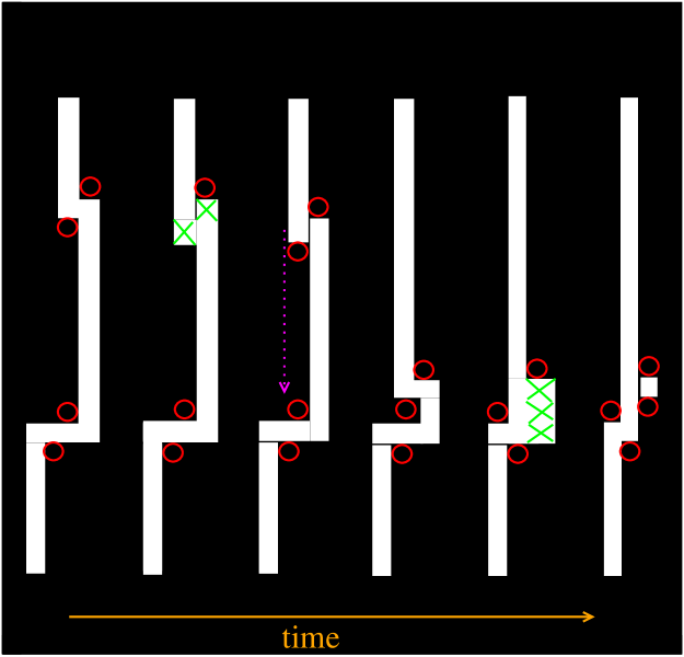
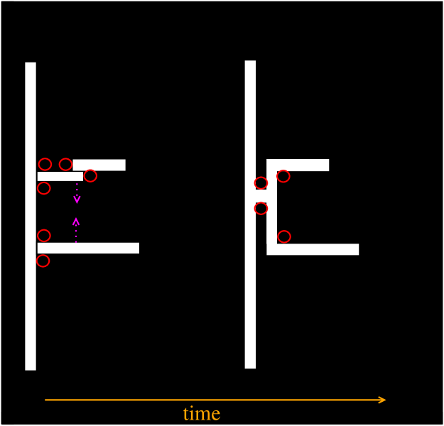
In this section we study the $p\to 1$ limit by letting $p=0.99$ in the numerical simulations. In the limit $p\to 1$, $\rho(t)$ still decays to zero, see Fig. 5. Hence, for large times there is a very small fraction of vacancies. Despite this fact, vacancies cannot be isolated, otherwise the dynamical constraints would freeze the system, which is not observed at any time in our simulations. These two requirements can be both fulfilled if vacancies segregate into quasi-unidimensional domains (see Fig. 8). A representation of a quasi-unidimensional domain is given in Fig. 9. Such a domain is basically a set of vacancies each of which is surrounded by $n=1,2$ neighbouring vacancies. The word quasi refers to the fact that these strings of vacancies can be seldom decorated by some bi-dimensional feature such as a traveling vacancy (TV), and $T$-junctions, as shown in Fig. 9. Since these objects are basically one-dimensional the system is allowed to build very long strings with a vanishing vacancy density in the thermodynamic limit.

Figure 8: (Color online.) Left and central panel: A zoom on the configuration of the system at two times ($t=10^{5}$ and $t=10^{7}$) after a quench to $p=0.99$. Black and white sites are frozen particles and vacancies, respectively. Red and green sites are particles and holes that can be updated. Right panel: Configuration of the system at time $t=10^{7}$ after a quench to $p=0.85$. The structure is fuzzier than in the $p=0.99$ case.

In the limit $p\to 1$ the dynamics proceed as follows: starting from a generic configuration at large times the only possible move is almost always the removal of a non frozen particle. This process takes a typical time $\tau_{0}\simeq(1-p)^{-1}$, which diverges as $p\to 1$. There is basically no evolution on time-scales shorter than $\tau_{0}$ which must be regarded, therefore, as the shortest time in the system. Whenever a particle is removed it is always possible to add a particle (in the site from which it was previously removed or in the neighbourhood) and this event almost always occurs for $p\to 1$. On the other hand, processes such as the consecutive removal of two (or more) particles, which have probability of order $(1-p)^{2}$ (or higher powers of $1-p$) can be discarded. Therefore we can focus on the leading events to lowest order in $1-p$ and the dynamics are provided by the following mechanisms (see Fig. 9)

• Diffusion and annihilation of traveling vacancies: with probability $1-p$ one of the particles surrounding a traveling vacancy can be removed. When this occurs a pair of adjacent TVs is formed and, since $p\simeq 1$, one of the two is immediately filled with a particle. This process, which taken alone does not change $\rho$, makes TVs diffuse along flat parts of the string. If two TVs come together one of them is immediately filled with a particle and $\rho$ decreases.

• Deformation around kinks or T-junctions: a particle can be removed with probability $1-p$ from the internal part of a kink or a T-junction. Hence the neighbouring site can be filled by a particle. This process produces the deformation of the string, since kinks and T-junctions can diffuse and/or generate new kinks and TVs. In addition, if two kinks or T-junctions meet, a new particle can be added lowering the density. Notice that these mechanisms, besides lowering the density, may give rise to the coalescence of strings, increasing the size of the quasi-unidimensional aggregates of vacancies, a phenomenon which is clearly observed in Fig. 8.

Figure 9: (Color online.) Schematic evolution of the system. Black sites are particles, (a red circle indicates the ones which are not frozen) white sites are vacancies (a green cross indicates those which are not frozen). Left panel: the mechanism producing the diffusion and annihilation of two TVs. Central panel: the mechanism producing the diffusion and coalescence of two kinks. Right panel: two T-junctions can diffuse similarly to kinks (see central panel) and merge.

As discussed above the deformation and coalescence between strings lead to a perpetual growth of the typical string length, and consequently of the average distance between strings $L(t)$, as can be observed in Fig. 8. This suggests that dynamical scaling may set in for large times, due to the prevalence of $L(t)$ over any other length, similarly to what happens in coarsening systems. According to the scaling hypothesis, configurations of the system look statistically similar if distances are measured in units of $L(t)$. For the equal time correlation function this implies $G(r,t)/G(0,t)=g(r/L(t))$. Similarly, the autocorrelation function must depend on $t,t_{w}$ only through the ratio $x=L(t)/L(t_{w})$, namely

$$\hat{C}(t,t_{w})=f(x)\qquad\mbox{with}\qquad x=\frac{L(t)}{L(t_{w})}$$ (14)

In the following we check this hypothesis.

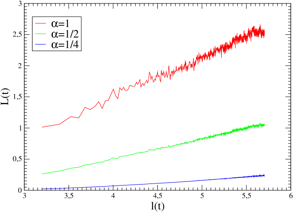
Due to the one-dimensional geometry of the strings, we expect the typical distance between them to be proportional to the inverse of the vacancy density $\rho_{v}(t)$. Since in this limit $\rho_{v}(t)=1-\rho(t)\simeq l^{-1}(t)$ we claim

$$L(t)\propto l(t).$$ (15)

This is demonstrated in Fig. 10 where we plot $L(t)$ computed through Eq. (12) for different values of $\alpha$ against $l(t)$. In the presence of scaling, as already observed in Sec. III, determinations of $L(t)$ using different values of $\alpha$ give the same result, apart from a multiplicative constant. Notice however that, in the presence of noise, the quality of the determination of $L(t)$ may strongly depend on the value of $\alpha$. Actually, different values of $\alpha$ weight differently regions with different $r$ and, since data at small $r$ are typically less noisy, smaller values of $\alpha$ lead to cleaner results. This is clearly observed in Fig. 10. On the other hand, if preasymptotic corrections to scaling are present, deviations from scaling can be enhanced or suppressed by changing $\alpha$, because those corrections may be more effective in the large or small $r$ regions, depending on the system. Actually, the data for $\alpha=1$ and $\alpha=0.5$ show no appreciable deviations from the asymptotic law $L(t)\propto l(t)$ in the whole time range; with $\alpha=0.25$ one observes small deviations up to $l(t)\simeq 4-4.5$ which can be interpreted as due to preasymptotic corrections to scaling. In any case, data for $l(t)>4.5$ clearly show that $L(t)\propto l(t)$ for all $\alpha$. This implies that scaling is obeyed and that, in this case, $l(t)$ has the meaning of a length.

Figure 10: (Color online.) The typical length defined in Eq. (12), for different values of $\alpha$ given in the key, against $l(t)$.

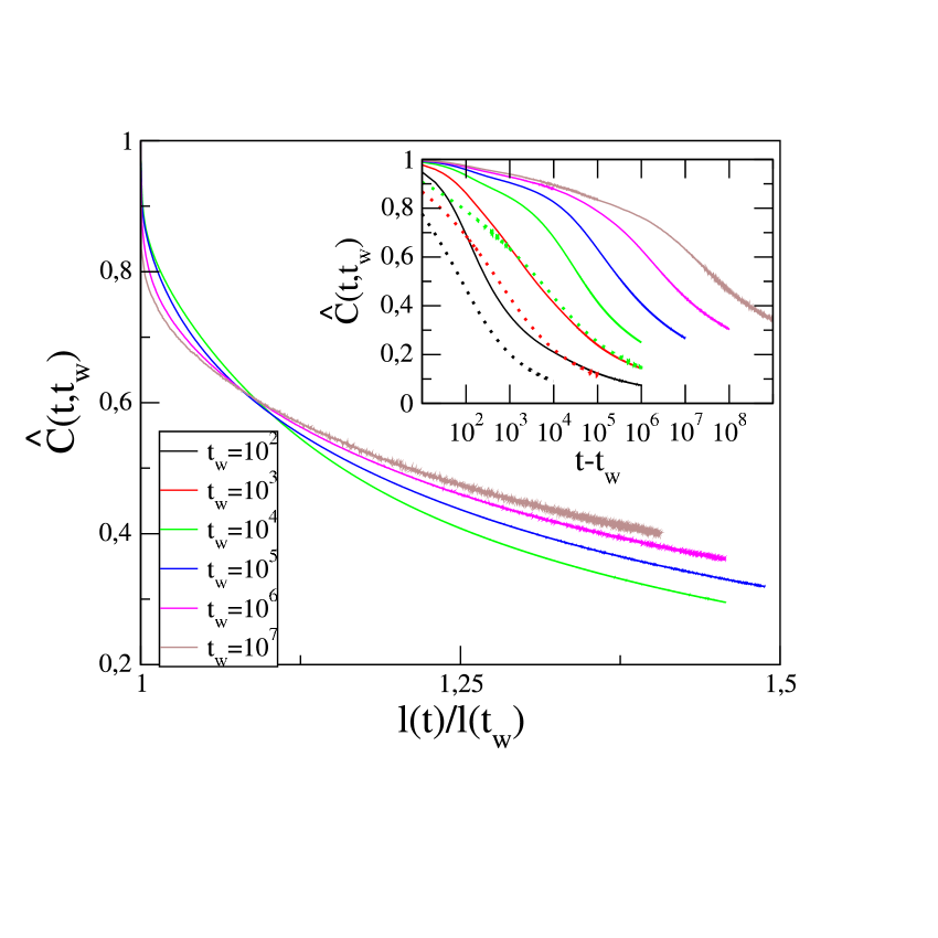
Since $G(r,t)$ is too noisy to obtain further evidence for scaling we consider in the following two-time quantities. In the inset of Fig. 11 we plot $\hat{C}(t,t_{w})$ against $t-t_{w}$ for different values of $t_{w}$. One clearly observes an aging behavior. The behaviour is very similar to the one in the $1d$ Ising chain. The apparent plateau slowly moves upwards and tends to $1$. In the main figure $\hat{C}(t,t_{w})$ is plotted against $l(t)/l(t_{w})$. Although the data collapse does not provide a definitive evidence for scaling, there is a clear improvement upon the collapse as $t_{w}$ increases, suggesting that scaling may be asymptotically obeyed for very large $t_{w}$. Interestingly all the curves intersect at the point of coordinate $x\simeq 1.08$ with curves for longer (shorter) $t_{w}$ lying below (above) curves for shorter (longer) $t_{w}$ before (after) the crossing point. This is somewhat similar to what was found in Monte Carlo simulations of the Sherrington-Kirkpatrick (SK) spin-glass Yoshino , that is known to satisfy dynamic ultrametricity asymptotically Cuku94 . However, in the spiral model the distance between consecutive curves reduces as $t_{w}$ increases (contrary to what is seen in the SK case) thus suggesting that this peculiar fact is just a pre-asymptotic effect.

Figure 11: (Color online.) The system is prepared in equilibrium at $p_{0}=0$ and then instantaneously quenched to $p=0.99$ at $t=0$. $\hat{C}(t,t_{w})$ is plotted against $l(t)/l(t_{w})$ for different values of $t_{w}$ given in the key. In the inset, the continuous lines are the same curves $\hat{C}(t,t_{w})$ of the main figure but plotted against $t-t_{w}$. The dotted lines represent $\hat{C}(t,t_{w})$ against $t-t_{w}$ (for different values of $t_{w}$ given by the same colour code of the continuous lines) after a quench to $p=0.85$.

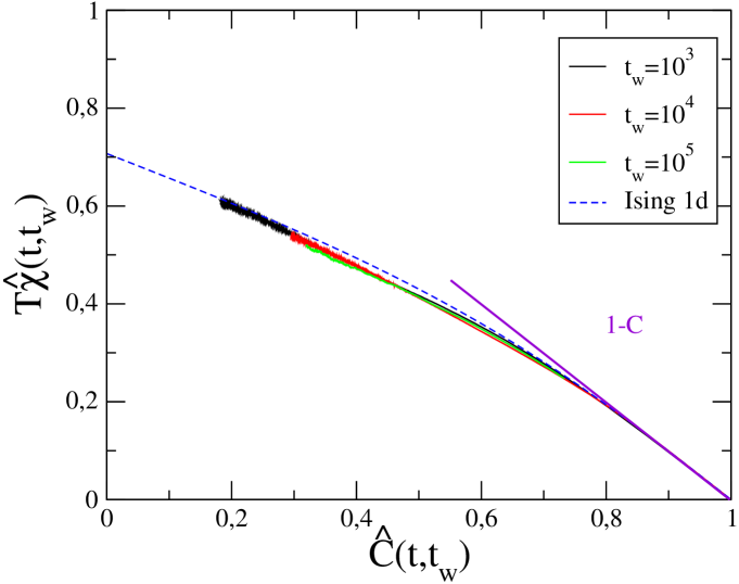
Next we consider the response function. In Fig. 12 the fluctuation dissipation plot $T\hat{\chi}(t,t_{w})$ against $\hat{C}(t,t_{w})$ is shown. The curves collapse quite well on a mastercurve $\widetilde{\chi}_{p\simeq 1}(\hat{C})$. This implies that the response function obeys the same scaling as $\hat{C}(t,t_{w})$, namely $\hat{\chi}(t,t_{w})=h(x)$ with $x=L(t)/L(t_{w})$. In the short time regime, for values of the $x$ axis that are close to one, one has $\tilde{\chi}(\hat{C})_{p\simeq 1}\simeq 1-\hat{C}$. As $\hat{C}$ decreases the curve bends. Although, naively, one could think that the parametric plot is one with two straight lines (one with the temperature of the bath and another one with a different value with a sharp crossover in between) the interpretation of the dynamics in terms of one dimensional coarsening suggests instead that the asymptotic construction is a non-trivial curve analogue to the one found in the $1d$ Ising model. Actually, as shown in Fig. 12, $\widetilde{\chi}_{p\simeq 1}(\hat{C})$ is quite similar to the parametric plot $\widetilde{\chi}_{T\simeq 0}(C)$ (known analytically 1dIM ) of $\chi$ vs $C$ in the $1d$ Ising model quenched to $T\simeq 0$ (no normalization is needed in this case since $C(t,t)=1$). Since $\widetilde{\chi}_{T\simeq 0}(C)$ is known not to be universal (depending, for instance on the observable used to compute the response sollich2 ) we do not expect the curves for the two models to be quantitatively equal, but only to behave in a qualitatively similar way. On the other hand, since the limiting slope $X_{\infty}=d\widetilde{\chi}_{T\simeq 0}(C)/dC|_{C=0}=1/2$ is expected to be universal xinfty ; Sollich , it would be interesting to compare this value with the limiting slope of the spiral model.

Figure 12: (Color online.) Left panel: $T\hat{\chi}(t,t_{w})$ against $\hat{C}(t,t_{w})$ for different values of $t_{w}$, in the case of an infinitely rapid quench from equilibrium at $p_{0}=0$ to $p=0.99$. The bold purple line is the equilibrium behavior $T\hat{\chi}(t,t_{w})=1-\hat{C}(t,t_{w})$. The dashed blue line is the parametric plot of $\chi$ vs $C$ in the $1d$ Ising model. Right panel: $T\hat{\chi}(t,t_{w})$ against $\hat{C}(t,t_{w})$ for $t_{w}=10^{3}$ in the case of an infinitely rapid quench from equilibrium at $p_{0}=0$ to different values of $p>p_{c}$ given in the key.

Quenches to $p_{c}<p<1$

In this Section we consider quenches from an empty state to $p_{c}<p<1$. With respect to the case $p\to 1$ considered above, there is now a non-vanishing annihilation probability, due to a finite $1-p$. Hence, after a time of order $\tau_{n}\simeq(1-p)^{-n}$, processes where $n$ vacancies are created start to be observed. Then, for $t<\tau_{2}$ the dynamics proceeds similarly to the case of a quench to $p\to 1$; later on a bubble of empty sites can be created around a quasi-dimensional structure, as can be seen in the right panel of Fig. 8. These processes produce a local rejuvenation of the system, since in the bubbles the density decreases (although globally it is still growing as shown in Fig. 5). As an effect, for a given $t_{w}$, the autocorrelation function decays faster than in the case with $p\to 1$, as can be seen in the inset of Fig. 11.

The process of bubble formation can be compared to the fast quasi-equilibrium processes occurring in ferromagnetic systems when quenched to a finite $T>0$. In scalar models (e.g. the Ising model) these processes are basically the reversal of spins in the bulk of ordered domains due to thermal fluctuations. In systems with a finite critical temperature $T_{c}$ (say, the Ising model in $d>1$) quenched below $T_{c}$, in the large-$t_{w}$ limit the timescale of fast processes is widely separated from the timescale over which irreversible or aging events occur. Quasi-equilibrium processes are responsible for the fast initial decay of $C(t,t_{w})$ to a plateau value $C(t,t_{w})=m^{2}$, namely the squared equilibrium magnetization, which occurs for $t-t_{w}<\tau_{eq}$, where $\tau_{eq}$ is the equilibrium relaxation time. Being equilibrium fluctuations in nature, these processes obey the FDT, and Eq. (7) is observed in a restricted time domain when $C(t,t_{w})\geq m^{2}$. Despite this fact, the system is globally aging, as shown by the further decay of $C(t,t_{w})$ from the plateau value on much larger timescales $t-t_{w}\gtrsim t_{w}\gg\tau_{eq}$ when aging processes become relevant. Notice that, by raising $T$ towards $T_{c}$ the region of the parametric plot where the FDT is observed extends to lower and lower values of $C$ until at $T_{c}$ Eq. (7) is obeyed in the whole range of $C$ variation. For system with $T_{c}=0$ (i.e. the $1d$ Ising model) quenched to a low $T>0$, instead, the appearance of thermal fluctuations in the bulk of domains at a certain time $t_{eq}$ is accompanied by the global equilibration of the system, so that aging is interrupted. Eq. (7) is then globally obeyed from $t_{w}\simeq t_{eq}$ onwards.

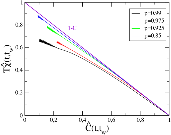
In the spiral model with $p<1$ bubble formation seems to play a role broadly similar to thermal fluctuations in ferromagnets, although combining features of systems with $T_{c}=0$ to those of the cases with $T_{c}>0$, and with some notable differences. Actually, when bubbles begin to be formed $\hat{C}(t,t_{w})$ starts to decay faster than in the case with $p\to 1$, but we could not detect the existence of a two step relaxation (with a plateau in between) in our data for $\hat{C}(t,t_{w})$ (see Fig. 11). This suggests that an effective time-scale separation between fast and slow processes as observed in ferromagnetic systems is not present in the spiral model, at least in the time sector studied in our simulations. In Fig. 12-right the parametric plot of $\hat{\chi}$ against $\hat{C}$ is shown for quenches to different values of $p>p_{c}$. Only the value $t_{w}=10^{3}$ is shown, we found that for each choice of $p$ the curves with values of $t_{w}$ up to $t_{w}=10^{5}$ are indistinguishable within numerical errors from the corresponding ones with $t_{w}=10^{3}$. Although we cannot exclude that a tiny $t_{w}$-dependence could be observed by considering much larger values of $t_{w}$, this strongly suggests that the curves with different $t_{w}$ collapse on a $p$-dependent mastercurve $\widetilde{\chi}_{p}(\hat{C})$. Notice that by lowering $p$ towards $p_{c}$, $\widetilde{\chi}_{p}(\hat{C})$ rises towards the FDT line (7) and the region of large $\hat{C}$ where the FDT is approximatively obeyed is enlarged. This is partly similar to what observed in ferromagnets with $T_{c}>0$ quenched below $T_{c}$ when $T$ is raised towards $T_{c}$. However, at variance with those systems, the shape of the plot is non trivial (i.e. all the curves bend continuously) and there is no apparent dependence on $t_{w}$, although from the inspection of $C$ one concludes that the system is still globally aging. These features resemble what observed in ferromagnets with $T_{c}=0$; in the spiral model however this behavior is observed in the whole glassy phase $p>p_{c}$.

VI Conclusions

At variance with most kinetically constrained spin models, the spiral model is characterized by an equilibrium glass-jamming transition at a finite value of the control parameter: for $p\geq p_{c}$ an infinite cluster of frozen particles exists. In view of the more general issue of glassy systems, therefore, it is of a certain interest to study and understand the effect and the relevance of such a transition on the non-equilibrium dynamical properties. In so doing we uncover a quite interesting and rich scenario with unexpected far from equilibrium features. Actually, while the equilibrium dynamics (and the near-to-equilibrium one of the annealing process considered in Sec. V.1) feels the presence of blocked regions the size of which diverges at the transition, leading to diverging relaxation times in the persistence function or in the autocorrelation, the non-equilibrium kinetics following an abrupt change of $p$, from below to above $p_{c}$, takes a completely different route avoiding the percolative blocked configurations relevant in equilibrium. At the basis of this behavior is the reversibility property of any kinetics obeying detailed balance. Due to this fact, a blocked configuration cannot be connected dynamically with an unblocked one. As a consequence, a system prepared initially in any state without a spanning frozen cluster keeps evolving on a restricted ensemble of configurations without such clusters. Evolution on a sub-ensemble of configurations (those with vanishing magnetization) is a key feature of coarsening systems. Actually, we found that the analogy between the spiral model and quenched ferromagnets goes beyond this. The non-equilibrium kinetics of the spiral model is actually a coarsening phenomenon where quasi-unidimensional strings of vacancies deform, diffuse and merge increasing their typical length $L(t)$ in a power-law fashion (logarithmically in the extreme case $p\to 1$). Observable quantities obey a dynamical scaling symmetry with $L(t)$ acting as a scale factor, much in the same way as in usual coarsening. Interestingly enough, the non-equilibrium fluctuation dissipation plot is a non trivial ($p$-dependent) curve, qualitatively similar to the one observed in the $1d$ Ising model. This feature may suggest that a similar mechanism is at work in the kinetics of the spiral model and of the Ising chain. It must be stressed, however, that in the former a non-trivial fluctuation-dissipation plot is observed in the whole glassy phase with $p>p_{c}$, and not only in a limiting sector of the phase diagram (i.e. $T\to 0$) as in the $1d$ Ising model, a feature resembling what is found in the Sherrington-Kirkpatrick spin-glass model Cuku94 .

Acknowlewdgements. We thank G. Biroli and Y. Shokef for very useful discussions. F.C. acknowledges financial support from PRIN 2007 JHLPEZ (Statistical Physics of Strongly correlated systems in Equilibrium and out of Equilibrium: Exact Results and Field Theory methods) and from CNRS and thanks the LPTHE Jussieu for hospitality during the preparation of this work. L.F. Cugliandolo is a member of Institut Universitaire de France.

References

- (1) G. H. Fredrickson and H. C. Andersen, Phys. Rev. Lett. 53, 1244 (1984).
- (2) J. Jäckle, J. Phys. Cond. Matt. 14, 1423 (2002).
- (3) P. Sollich and F. Ritort, Adv. in Phys. 52, 219 (2003).
- (4) For a review see S. Leonard, P. Mayer, P. Sollich, L. Berthier, and J. P. Garrahan, J. Stat. Mech. P07017 (2007).
- (5) G. H. Fredrickson and S. A. Brawer, J. Chem. Phys. 84, 3351 (1986).
- (6) I. S. Graham, L. Piché, and M. Grant, Phys. Rev. E 55, 2132 (1997).
- (7) W. Kob and H. C. Andersen, Phys. Rev. E 48, 4364 (1993). J. P. Garrahan and D. Chandler, Phys. Rev. Lett. A. C. Pan, J. P. Garrahan, and D. Chandler, Phys. Rev. E 72, 041106 (2005).
- (8) P. Harrowell, Phys. Rev. E 48, 4359 (1993). L. Berthier, D. Chandler, and J. P. Garrahan, Europhys. Lett. 69, 320 (2005). A. C. Pan, J. P. Garrahan, and D. Chandler, Chem. Phys. Chem. 6, 1783 (2005).
- (9) G. H. Fredrickson and S. A. Brawer, J. Chem. Phys. 84, 3351 (1986). G. H. Fredrickson, Annals NY Acad. of Sci. 484, 185, (1986). J. Kurchan, L. Peliti, and M. Sellitto M, Europhys. Lett. 39, 365 (1997).
- (10) M. Sellitto, Euro. Phys. J. B 4, 135 (1998). R. L. Jack, L. Berthier, and J. P. Garrahan, J. Stat. Mech. P12005 (2006).
- (11) L. F. Cugliandolo and J. Kurchan, Phys. Rev. Lett. 71, 173 (1993).
- (12) L. F. Cugliandolo, J. Kurchan, and L. Peliti, Phys. Rev. E 55, 3898 (1997).
- (13) C. Chamon, P. Charbonneau, L. F. Cugliandolo, D. R. Reichman, and M. Sellitto, J. Chem. Phys. 121, 10120 (2004).
- (14) C. Toninelli, G. Biroli, and D. S. Fisher, Phys. Rev. Lett. 92, 185504 (2004).
- (15) J. Reiter, F. Mauch and J. Jäckle, Physica A 184, 458 (1992). S. J. Pitts, T. Young, and H. C. Andersen, J. Chem. Phys. 113, 8671 (2000). M. Sellitto, G. Biroli, and C. Toninelli, Europhys. Lett. 69, 496 (2005).
- (16) G. Biroli and C. Toninelli, Eur. Phys. J. B 64, 567 (2008).
- (17) C. Toninelli and G. Biroli, J. Stat. Phys. 130, 83-112 (2008).
- (18) C. Toninelli, G. Biroli, and D. S. Fisher, Phys. Rev. Lett. 96 035702 (2006).
- (19) C. Toninelli, G. Biroli, and D. S. Fisher, Phys. Rev. Lett. 98 129602 (2008).
- (20) R.G. Palmer, Adv. Phys. 31, 669 (1982). J. Kurchan and J. Laloux, J. Phys. A 29, 1929 (1996). C.M. Newman and D.L. Stein, J. Stat. Phys. 94, 709 (1999).
- (21) G. Szamel, J. Chem. Phys. 121, 3355 (2004).
- (22) E. Lippiello, F. Corberi and M. Zannetti, Phys. Rev. E 71, 036104 (2005).
- (23) A. Cavagna, Supercooled Liquids for Pedestrians arXiv:0903.4264, Phys. Rep. (to appear).
- (24) A. Montanari and F. Ricci-Tersenghi, Phys. Rev. B 70, 134406 (2004).
- (25) C. Godrèche and J-M Luck, E. Lippiello and M. Zanetti,
- (26) S. Franz and G. Parisi, J. Physique I 5, 1401 (1995). A. Barrat, R. Burioni, and M. Mézard, J. Phys. A 29, L81 (1996). L. F. Cugliandolo, J. Kurchan, P. Le Doussal, and L. Peliti, Phys. Rev. Lett. 78, 350 (1997).
- (27) C. Godrèche and J-M Luck, J. Phys.: Cond. Matt. 14, 1589 (2002).
- (28) P. Sollich, S. Fielding, and P. Mayer, J. Phys.: Cond. Matt. 14, 1683 (2002). P. Mayer, L. Berthier, J.P. Garrahan, and P. Sollich, Phys. Rev. E 68, 016116 (2003).
- (29) H. Takayama, H. Yoshino, and K. Hukushima J. Phys. A 30, 3891 (1997).
- (30) L. F. Cugliandolo and J. Kurchan, J. Phys. A 27, 5749 (1994).