Complex network approach for recurrence analysis of time series
Abstract
We propose a novel approach for analysing time series using complex network theory. We identify the recurrence matrix (calculated from time series) with the adjacency matrix of a complex network and apply measures for the characterisation of complex networks to this recurrence matrix. By using the logistic map, we illustrate the potential of these complex network measures for the detection of dynamical transitions. Finally, we apply the proposed approach to a marine palaeo-climate record and identify the subtle changes to the climate regime.
keywords:
recurrence plot , complex networks , dynamical transitions , palaeo-climatePACS:
05.40.-a , 05.45.-a , 05.45.Tp , 91.10.Vr , 91.50.Jc1 Introduction
In many scientific disciplines, such as engineering, astrophysics, life sciences and economics, modern data analysis techniques are becoming increasingly popular as a means of understanding the underlying complex dynamics of the system. Methods for estimating fractal or correlation dimensions, Lyapunov exponents, and mutual information have been widely used [1, 2, 3, 4]. However most of these methods require long data series and in particular their uncritical application, especially to real-world data, may often lead to pitfalls.
In the last two decades, the method of recurrence plots has been developed as another approach to describe complex dynamics [5]. A recurrence plot (RP) is the graphical representation of a binary symmetric square matrix which encodes the times when two states are in close proximity (i.e. neighbours in phase space). Based on such a recurrence matrix, a large and diverse amount of information on the dynamics of the system can be extracted and statistically quantified (using recurrence quantification analysis, dynamical invariants, etc.). Meanwhile this technique has been the subject of much interest from various disciplines [6] and it has been successfully applied to a number of areas: the detection of dynamical transitions [7, 8] and synchronisation [9], the study of protein structures [10, 11] and in cardiac and bone health conditions [12, 13], in ecological regimes [14, 15], economical dynamics [16, 17], in chemical reactions [18] and to monitor mechanical behaviour and damages in engineering [19, 20], to name a few. It is important to emphasise that recurrence plot based techniques are even useful for the analysis of short and non-stationary data, which often presents a critical issue when studying real world data. The last few years have witnessed great progress in the development of RP-based approaches for the analysis of complex systems [5, 21, 22, 23, 24].
During the last decade, complex networks have become rather popular for the analysis of complex and, in particular, spatially extended systems [25, 26, 27, 28]. Local and global properties (statistical measures) of complex networks are helpful to understand complex interrelations and information flow between different components in extended systems, such as social, computer or neural networks [25], food webs, transportation networks, power grids [29], or even in the global climate system [30]. The basis of complex network analysis is the adjacency matrix, representing the links between the nodes of the network. Like the recurrence matrix, the adjacency matrix is also square, binary, and symmetric (in the case of an unweighted and undirected network).
In fact, the recurrence matrix and the adjacency matrix exhibit a strong analogy: a recurrence matrix represents neighbours in phase space and an adjacency matrix represents links in a network; both matrices embody a pair-wise test of all components (phase space vectors resp. nodes). Therefore, we might well proceed to explore further analogies even in the statistical analysis of both the recurrence and the adjacency matrix.
Quantitative descriptors of RPs have been first introduced in a heuristic way in order to distinguish different appearances of RPs [6]. We may also consider to apply measures of complex network theory to a RP in order to quantify the RP’s structure and the corresponding topology of the underlying phase space trajectory. In this (more heuristic) sense, it is actually not necessary to consider the phase space trajectory as a network.
Recently, the very first steps in the direction of bridging complex network theory and recurrence analysis have been reported [32, 31]. In these works, the local properties of phase space trajectories have been studied using complex network measures. Zhang et al. suggested using cycles of the phase space trajectory as nodes and considering a link when two cycles are rather similar [32, 33]. The resulting adjacency matrix can be in fact interpreted as a special recurrence matrix. The recurrence criterion here is the matching of two cycles. A complementary approach was suggested by Xu et al. who studied the structural shape of the direct neighbourhood of the phase space trajectory by a motif classification [31]. The adjacency matrix of the underlying network corresponds to the recurrence matrix, using the recurrence criterion of a fixed number of neighbours (instead of the more often used fixed size of the neighbourhood [5]).
Other approaches for the study of time series by a complex network analysis suggested using linear correlations [34] or another certain condition on the time series amplitudes (“visibility”) [35].
In this letter, we demonstrate that the recurrence matrix (analogously to [31]) can be considered as the adjacency matrix of an undirected, unweighted network, allowing us to study time series using a complex network approach. This ansatz on creating complex network is more natural and simple than the various suggested approaches [33, 34, 35]. Complex network statistics is helpful to characterise the local and global properties of a network. We propose using these complex network measures for a quantitative description of recurrence matrices. By applying these measures, we obtain additional information from the recurrence plots, which can be used for characterising the dynamics of the underlying process. We give an interpretation of this approach in the context of the dynamics of a phase space trajectory. Nevertheless, many of these measures neither have an analogue in traditional RQA nor in nonlinear time series analysis in a wider sense, and hence, open up new perspectives for the quantitative analysis of dynamical systems. We illustrate our approach with a prototypical model system and a real-world example from the Earth sciences.
2 Recurrence plots and complex networks
A recurrence plot is a representation of recurrent states of a dynamical system in its -dimensional phase space. It is a pair-wise test of all phase space vectors () among each other, whether or not they are close:
| (1) |
with being the Heaviside function and a threshold for proximity [5]. The closeness can be measured in different ways, by using, e.g., spatial distance, string metric, or local rank order [5, 36]. Mostly, a spatial distance is considered in terms of maximum or Euclidean norm . The binary recurrence matrix contains the value one for all close pairs . A phase space trajectory can be reconstructed from a time series by time delay embedding [37]
| (2) |
where is the embedding dimension and is the delay.
The resulting matrix exhibits the line of identity (the main diagonal) . Using a spatial distance as the recurrence criterion, the RP is symmetric. Small-scale features in a RP can be observed in terms of diagonal and vertical lines. The presence of such lines reflects the dynamics of the system and is related to divergence (Lyapunov exponents) or intermittency [7, 12, 24]. Following a heuristic approach, a quantitative description of RPs based on these line structures was introduced and is known as recurrence quantification analysis (RQA) [6]. We use the following two RQA measures (a comparable study using other measures can be found in [12]).
Similarly evolving epochs of the phase space trajectory cause diagonal structures parallel to the main diagonal. The length of such diagonal line structures depends on the predictability and, hence, the dynamics of the system (periodic, chaotic, stochastic). Therefore, the distribution of diagonal line lengths can be used for characterising the system’s dynamics. Several RQA measures are based on . However, here we focus only on the maximal diagonal line length,
| (3) |
where is the total number of diagonal lines. For the definition of a diagonal line, we use a minimal length [5]. The length of diagonal lines corresponds to the predictability time. In particular, the cumulative distribution of the line lengths can be used to estimate the correlation entropy , i.e. the lower limit of the sum of the positive Lyapunov exponents [5]. Hence the inverse of gives a first rough impression of the divergence (Lyapunov exponent) of the system.
Slowly changing states, as occurring during laminar phases (intermittency), result in vertical structures in the RP. Therefore, the distribution of vertical line lengths can be used to quantify laminar phases occurring in a system. A useful measure for quantifying such laminar phases is the ratio of recurrence points forming vertical structures to all recurrence points,
| (4) |
which is called laminarity [5].
Now let us consider the phase space vectors as nodes of a network and identify recurrences with links. An undirected and unweighted network is represented by the binary adjacency matrix , where a connection between nodes and is marked as . Excluding self-loops, we obtain from the RP by removing the identity matrix,
| (5) |
where is the Kronecker delta. Removing the identity is not a problem, as this is also done in the analysis of RPs (e.g. when considering a Theiler window for RQA) [5]. Henceforth, we regard the recurrence matrix (with applied Theiler window) to be an adjacency matrix. Note that this way each state vector in phase space is represented by one distinct node; even if two time-separated state vectors are identical, they are identified with two different nodes (which are perfect neighbours and therefore linked independently of the threshold ; such nodes are also called twins [38]).
Local and global properties of a network are statistically described by complex network measures based on the adjacency matrix . To illustrate the potential of a recurrence analysis by means of complex network theory, we consider several global and local network measures that are well studied in literature [27].
The complex network approach allows to harness the distributions of locally defined measures for the quantification of recurrence matrices. In this work, we particularly consider the degree centrality
| (6) |
giving the number of neighbours of node . The degree centrality is hence locally defined and depends only on local adjacency information in a topological sense. is proportional to the local recurrence rate, as seen from a RQA point of view. Hence, it may be considered as a measure for the local phase space density. We refer to its frequency distribution as the degree distribution.
Furthermore, a complex network may be globally described by its link density, clustering coefficient and average path length. While the normalised averaged degree centrality, called link density,
| (7) |
corresponds to the global recurrence rate, the latter two measures allow quantifying novel aspects of recurrence matrices. The clustering coefficient gives the probability that two neighbours (i.e. recurrences) of any state are also neighbours [25]. It is obtained as the average of the local clustering coefficient
| (8) |
The average length of shortest paths between all pairs of nodes is given by the average path length
| (9) |
where the length of a shortest path is defined as the minimum number of links that have to be crossed to travel from node to node [27]. Disconnected pairs of nodes are not included in the average (for a detailed discussion see [39]). Note that it is particularly interesting to study clustering coefficient and average path length in unison, since both measures taken together allow to characterise “small-world” behaviour in complex networks [25]. In a separate study, we link the properties of a complex network with the topology of a phase space representation of a dynamical system in more detail [40]. In particular, a complex network based on a recurrence plot usually does not exhibit the small-world feature, since graph distances are directly related to distances in phase space (i.e. there are no “shortcuts” between distant nodes).
3 Application to logistic map
We illustrate the potential of the proposed approach by an analysis of the logistic map
| (10) |
especially within the interesting range of the control parameter with a step size of . In the analysed range of , various dynamic regimes and transitions between them can be found, e. g., accumulation points, periodic and chaotic states, band merging points, period doublings, inner and outer crises [41, 42, 43]. This system has been used to illustrate the capabilities of RQA. It was shown that diagonal line based RQA measures are able to detect chaos-order transitions [7] and vertical line based measures even detect chaos-chaos transitions [12].
Since Eq. (10) is a one-dimensional map, we compute the RP without embedding. For the study of transitions, it is recommended to use a recurrence threshold preserving a fixed recurrence rate, say 5%. However, in the special case of the logistic map, such approach leads to problems within the periodic windows. In these windows the states are rapidly alternating between subsequent time steps, leading to a high recurrence rate (larger than 25%). Therefore, a threshold for preserving 5% recurrence rate does not exist and, hence, we cannot compute the network measures within the periodic windows. To circumvent this, we will use a fixed recurrence threshold for the example of the logistic map (for the real world example in Sect. 4, we will use the preferred criteria of constant recurrence rate). The threshold is selected to be 5% of the standard deviation of the time series [52].
For periodic dynamics, band merging, laminar states (cross points of supertrack functions, cf. [12]), and outer crisis, we investigate the network measures in more detail (Tab. 1). The band merging corresponds to intermittency, the inner crisis to certain chaos-chaos transition and the outer crisis to fully chaotic dynamics (all these transitions are chaos-chaos transitions).
For these four cases, we compute a time series of length . In order to exclude transient responses we remove the leading values from the data series in the following analysis (thus we use values).
| Regime | ||||||
|---|---|---|---|---|---|---|
| period-3 | 3.830 | 8996 | 0 | 1 | 1 | 0.333 |
| band merging | 3.679 | 49 | 0.42 | 22.8 | 0.83 | 0.050 |
| laminar | 3.791 | 39 | 0.12 | 23.3 | 0.79 | 0.040 |
| outer crisis | 4.000 | 23 | 0.20 | 23.6 | 0.82 | 0.046 |
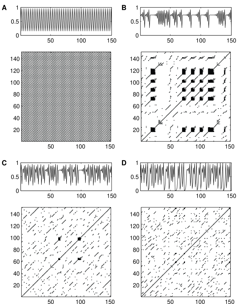
The recurrence plots for the four different dynamical regimes exhibit different typical characteristics of regular, laminar and chaotic dynamics (Fig. 1). In the periodic regime, , the RP consists only of non-interrupted diagonal lines (Fig. 1A). Their distance is 3, corresponding to the period length of 3 for this periodic regime. At the band merging point, , the RP reveals extended clusters of recurrence points, corresponding to many laminar phases (Fig. 1B). Moreover, several diagonal lines appear, showing short epochs of similar evolution of the states. The RP for laminar states, , consists also of (even though less) extended clusters, but possesses more diagonal lines (Fig. 1C). For the outer crisis, , diagonal lines appear but are shorter than those appearing for smaller (Fig. 1D), which is consistent with the Lyapunov exponent being largest for (with respect to smaller ).
The two RQA measures and confirm these visual observations (Tab. 1). For the period-3 regime, we find the longest diagonal lines (, after consideration of the Theiler window [44]). The maximal length of diagonal lines decreases for increasing control parameter . As expected, laminarity takes the highest value at the band merging point () with , but is lowest for the period-3 regime, . At intersections of supertrack functions, the laminarity is slightly increased (), and at the outer crisis the intermittency increases apparently ().
The complex network measures also highlight differences in the topological structure of these dynamical regimes (Tab. 1).
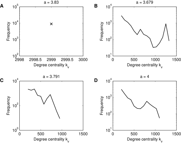
In the period-3 regime (), the observed values jump between three distinct states. These three states are isolated in phase space and are not considered to be neighbours (in the sense of the recurrence definition). Therefore, in the sense of a complex network, we have three disconnected components where each component contains a fully connected network (because all the nodes in each component represent the same state in phase space). The average shortest path length between nodes (i.e. states) should therefore be one, and the clustering is perfect. The average path length derived from the corresponding RP has indeed the smallest possible value (), and the clustering coefficient takes its largest possible value (). The degree centrality takes only one value: 2999 (Fig. 2A). This value corresponds approximately to a third of the size of the network, due to its partition by the period-3 cycles, which is confirmed by the link density ().
For the band merging (), we find and . The degree distribution has a multimodal shape (Fig. 2B), which implies that there are several states acting like super-nodes (i.e. which exhibit many links). These states lie at the merging point of the two bands (around ) and at the upper and lower border of the state space, i.e. in regions with high phase-space density (Fig. 3A). The link density is .
For the laminar state at , we find and . The degree centrality follows a distribution with slight bimodality (Fig. 2C). The resulting link density approaches its lowest value within the four considered dynamical regimes ().
Finally, for the outer crisis (), we obtain and . The degree centrality displays similar properties as for the laminar state, but with higher average values and a resulting link density of (Fig. 2D).
From the above results, we conclude that complex network measures applied to a recurrence matrix are indeed sensitive to changes in the dynamics. The average shortest path length can be considered as an upper bound for the phase space distance between two states (in units of the threshold value ). Hence, its average value can be interpreted as a mean distance, which depends on the total diameter and the fragmentation of the phase space. Therefore, increases with growing phase space of the logistic map (with growing control parameter ). The clustering coefficient is able to detect clustered phase vectors, as they appear in periodic or laminar dynamics. The degree centrality quantifies the phase-space density in the direct neighbourhood of a state , while the link density measures the average phase space density. Moreover, from the distribution we can infer that the considered recurrence matrices are not scale-free in the sense of the network theory.
Now we calculate , , , , , and for different values of the control parameter within the range . For each value of , we compute a time series of length , and exclude transients by removing the first values.
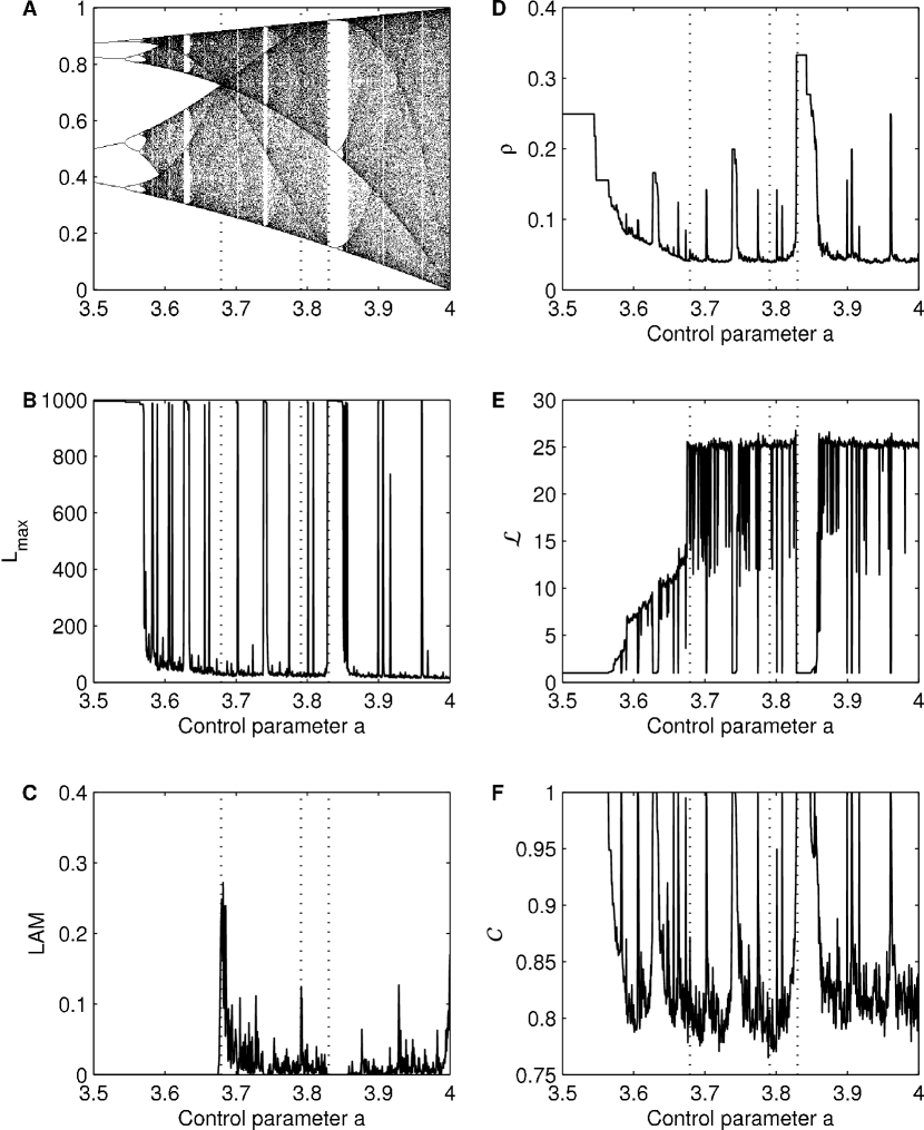
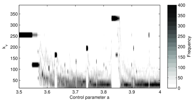
The RQA measure reveals periodic dynamics by maxima of its value (Fig. 3B). Laminar phases are clearly detected by (Fig. 3C). and also show maxima during episodes of periodic dynamics (Figs. 3D and F). corresponds to the recurrence rate and confirms previous studies [7]. Its values also depend on the periodicity during the periodic windows – the higher the periodicity, the lower . Therefore, period-doublings cause an abrupt decrease of this measure. In the periodic regime, neighbours of a state are equal to the state itself, leading to the largest possible clustering coefficient , and to the shortest possible path lengths between neighbours giving . However, shows a more interesting behaviour. In our interpretation of a recurrence matrix, characterises not only the total phase space diameter, but also its fragmentation. With respect to the logistic map, each time two bands in phase space merge (e.g. at or ), this does not only lead to an increase of the occupied phase space, but also yields a merging of formerly disjoint network clusters. As the definition of the average path length does not consider pairs of points in disconnected clusters, the average distance of connected nodes suddenly increases shortly before the band merging point as soon as the distance between the different bands falls below , since the clusters then become connected. This is clearly expressed by jumps in (Fig. 3E). The distribution of is discrete in the periodic windows, which are therefore clearly identifiable (Fig. 4). Analogous to the link density , the location of the maxima of the degree distribution in periodic windows is related to the number of periods, e.g., for period-4 we have , for period-3 (for a time series length of ). The degree distribution before the band merging point is broad and reveals higher degrees than after the band merging point, which again relates to the connection of the distinct network clusters. For increased control parameter , becomes more localised around small degrees, disclosing the decrease of recurrences due to the increasingly chaotic behaviour (increasing Lyapunov exponent).
4 Application to marine dust record
Long-term variations in aeolian dust deposits are related to changes in terrestrial vegetation and are often used as a proxy for changing climate regimes in the past. For example, marine terrigenous dust records can be used to infer epochs of arid continental climate. In particular, a marine record from the Ocean Drilling Programme (ODP) derived from a drilling in the Atlantic, ODP site 659, was used to infer changes in African climate during the last 4.5 Ma (Fig. 5A) [45]. This time series has a length of with an average sampling time of 4.1 ka. Applying spectral analysis to these data, it was claimed that the African climate has shifted towards arid conditions at 2.8, 1.7 and 1.0 Ma before present (BP) [46]. These transitions correspond to epochs of different dominant Milankovich cycles (mid-Pleistocene transition with a “41 ka world” between 2.7 and 1.0 Ma BP and a “100 ka world” since about 1.0 Ma BP), the end of the Early Pliocene Warm Period at about 2.8 Ma BP, and the development of the Walker circulation around 1.9–1.7 Ma BP [47]. However, a recent thorough investigation of several marine dust records demonstrated more complex relationships between vegetational coverage, aeolian transport processes and the dust flux record [48]. The analysis revealed transitions between different regimes of variability, mostly driven by a variation of the solar irradiation due to different dominant Milankovich cycles. For example, Trauth et al. found an interval of a dominant 100 ka frequency (related to orbital eccentricity) between 3.2 and 3.0 Ma BP, and of dominant 19–23 ka frequency band (precession) between 2.3 and 2.0 Ma BP [48]. The Early Pliocene Warm Period ended between 3.3 and 2.8 Ma BP with the Pliocene optimum (3.24–3.05 Ma BP) and the onset of the northern hemisphere glaciation (2.8–2.7 Ma BP) [49, 47], which was intensified during the mid-Pleistocene climate shift at 1.0–0.7 Ma BP [50]. It has been hypothesised that the latter transition was connected with a period of strong Walker circulation between 1.5–0.5 Ma BP [51].
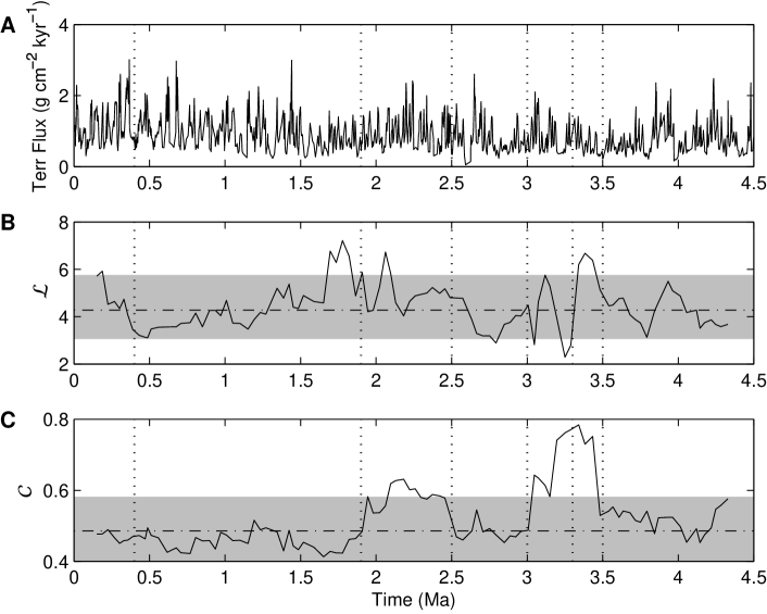
We illustrate the capabilities of our recurrence analysis using complex network measures for the ODP 659 dust flux record in order to find transitions in the dynamics. For this purpose, we use a time delay embedding with dimension and delay (these parameters have been determined by applying the standard procedure using false nearest neighbours and mutual information [1]). The threshold is chosen to preserve a constant recurrence rate of 5% (which means that the link density will be constant) [5, 52]. In order to study transitions in the dust record, we calculate the recurrence matrix in moving windows of size 100 time points (corresponding approximately to 410 ka) and with an overlap of 90%. For the time-scale of the windowed measurements, we use the mid-point of the window. Note that the time-scale is not equidistant (equidistant time-scale is not necessary for our network approach). On average, the sampling time is 4.1 ka with a standard deviation of ka. Compared to the long (geological) scale this deviation is still rather small. However, the application of linear methods often requires equidistant time-scales.
We will apply a simple statistical test in order to test the null-hypothesis to see whether the network characteristics at a certain time differs from the general network characteristics. In order to create an appropriate null-model, we use the following approach. In contrast to the RQA measures, where the time-ordering is important requiring a more advanced approach for a statistical test [53], for the network measures we can simply randomise the time series: we randomly draw 100 values (corresponding to the window size of 100 points) from the time series and then calculate the RP and the network measures from this sample. By repeating this 10,000 times we get a test distribution for the measures and and estimate its 0.05 and 0.95 quantiles that may be interpreted as the 90% confidence bounds.
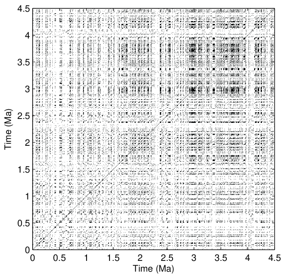
The RP of the dust data depicts a rather homogeneous recurrence structure, interrupted only by rather small bands of sparse recurrence point density (Fig. 6). Such sparse areas mark epochs of more frequently occurring extreme or rare events recorded by the marine dust data series. On the small-scale we find mostly very short diagonal lines, expressing the high variability and fast change of the states (with respect to the geological time-scale). Between 4.0 and 3.0 Ma and around 2.0 Ma BP, longer diagonal lines appear. Moreover, between 4.5 and 3.0 Ma BP, we find an increased number of vertical/ horizontal lines, indicating different dynamics than at other times.
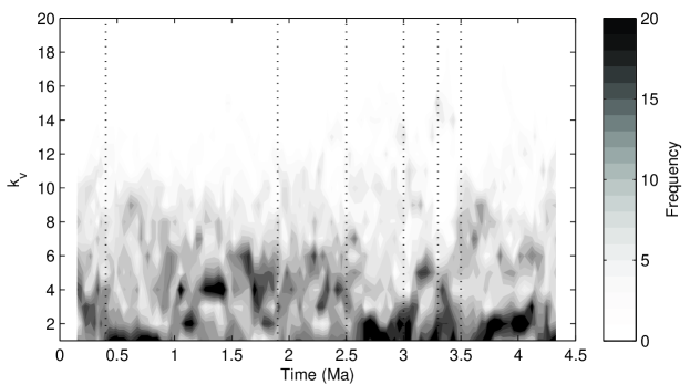
The global network measures and also depict a distinct variability (Fig. 5B and C). reveals epochs of significantly higher values between 3.5 and 3.3, , 1.9–1.8, and after 0.4 Ma BP. Around 3.3, 2.0 and 1.9 Ma BP the RP exhibits sudden drops of within a period of, in general, higher values. discloses epochs of increased values between 3.5 and 3.0 Ma as well as between 2.5 and 2.0 Ma BP. Between 4.5 and 3.5 Ma, 3.0 and 2.5 Ma, and 1.0 and 0.4 Ma BP, the degree centrality possesses mostly small values, whereas between 2.5 and 1.0 Ma and after 0.4 Ma BP, it has larger values (Fig. 7).
With respect to the previously known results, we conclude that identifies the epochs of more dominant Milankovich cycles (between 3.2 and 3.0 Ma and 2.3 and 2.0 Ma BP). is increased in these periods, but also exhibits increased values for the period between 2.5 and 1.0 Ma BP. Note that the 3.5-3.0 Ma BP period is related to the intensification of the Northern hemisphere glaciation [54]. In contrast, reveals transitions in climate dynamics on a different time-scale. Maxima of this measure tend to appear at the onset of changes in . Whereas reveals the changed dynamics, is sensitive to the transition periods, which is consistent with our results near the band-merging points of the logistic map. The increase of at , , 1.9–1.8, and 0.4 Ma BP may also be related to the intensification of glaciation. However, the detected transitions are associated with different and more subtle dynamical changes, and not simply just an intensification of a certain Milankovich cycle.
5 Conclusions
We have linked the recurrence matrix with the adjacency matrix of a complex network, and have proposed the direct application of the corresponding network measures to the recurrence matrix. We have discussed the link density, degree centrality, average path length and clustering coefficient in some detail. In particular, the latter two complex network measures have no direct counterpart in recurrence quantification analysis and give additional insights into the recurrence structure of dynamical systems. In a further study, we have outlined the link between the complex network measures and the properties of the phase space trajectory of dynamical systems [40].
By applying our novel approach to the logistic map, we have illustrated the ability of the proposed measures to distinguish between the different dynamical regimes and to detect the corresponding transitions. Moreover, we have used our approach to investigate a marine climate proxy record representing the climate variability over Africa during the last 4.5 Ma. The different measures highlighted various transitions in the recurrence structure and, hence, in the dynamics of the studied climate system. By applying the recurrence approach and complex network measures, we were able to identify more subtle transitions than those that were previously reported from using linear approaches, like power spectral analysis [46], linear trend detection [49], Mann-Whitney or Ansari-Bradley tests [48]. In addition, our proposed approach to detect transitions on the basis of time series does not require equidistant time-scales, as would be necessary for most other known techniques. From the network point of view, the recurrence plot approach can deliver a potential measure of information exchange in time series of complex systems [55, 40].
In the future, recurrence plots and their complex network interpretation will allow for further fruitful and natural transfer of ideas and techniques from complex network theory to time series analysis (and vice versa).
6 Acknowledgements
This work was partly supported by the German Research Foundation (DFG) project He 2789/8-2, SFB 555 project C1, and the Japanese Ministry for Science and Education.
References
- Kantz and Schreiber [1997] H. Kantz, T. Schreiber, Nonlinear Time Series Analysis, University Press, Cambridge, 1997.
- Kurths and Herzel [1987] J. Kurths, H. Herzel, An attractor in a solar time series, Physica D 25 (1987) 165–172, doi:10.1016/0167-2789(87)90099-6.
- Mandelbrot [1982] B. B. Mandelbrot, The fractal geometry of nature, Freeman, San Francisco, 1982.
- Wolf et al. [1985] A. Wolf, J. B. Swift, H. L. Swinney, J. A. Vastano, Determining Lyapunov Exponents from a Time Series, Physica D 16 (3) (1985) 285–317, doi:10.1016/0167-2789(85)90011-9.
- Marwan et al. [2007a] N. Marwan, M. C. Romano, M. Thiel, J. Kurths, Recurrence Plots for the Analysis of Complex Systems, Physics Reports 438 (5–6) (2007a) 237–329, doi:10.1016/j.physrep.2006.11.001.
- Marwan [2008] N. Marwan, A Historical Review of Recurrence Plots, European Physical Journal – Special Topics 164 (1) (2008) 3–12, doi:10.1140/epjst/e2008-00829-1.
- Trulla et al. [1996] L. L. Trulla, A. Giuliani, J. P. Zbilut, C. L. Webber Jr., Recurrence quantification analysis of the logistic equation with transients, Physics Letters A 223 (4) (1996) 255–260, doi:10.1016/S0375-9601(96)00741-4.
- Ngamga et al. [2007] E. J. Ngamga, A. Nandi, R. Ramaswamy, M. C. Romano, M. Thiel, J. Kurths, Recurrence analysis of strange nonchaotic dynamics, Physical Review E 75 (3) (2007) 036222, doi:10.1103/PhysRevE.75.036222.
- Romano et al. [2005] M. C. Romano, M. Thiel, J. Kurths, I. Z. Kiss, J. Hudson, Detection of synchronization for non-phase-coherent and non-stationary data, Europhysics Letters 71 (3) (2005) 466–472, doi:10.1209/epl/i2005-10095-1.
- Giuliani et al. [2002] A. Giuliani, R. Benigni, J. P. Zbilut, C. L. Webber Jr., P. Sirabella, A. Colosimo, Nonlinear Signal Analysis Methods in the Elucidation of Protein Sequence-Structure Relationships, Chemical Reviews 102 (5) (2002) 1471–1492, doi:10.1021/cr0101499.
- Zbilut et al. [2004] J. P. Zbilut, A. Giuliani, A. Colosimo, J. C. Mitchell, M. Colafranceschi, N. Marwan, V. N. Uversky, C. L. Webber Jr., Charge and Hydrophobicity Patterning along the Sequence Predicts the Folding Mechanism and Aggregation of Proteins: A Computational Approach, Journal of Proteome Research 3 (2004) 1243–1253, doi:10.1021/pr049883+.
- Marwan et al. [2002] N. Marwan, N. Wessel, U. Meyerfeldt, A. Schirdewan, J. Kurths, Recurrence Plot Based Measures of Complexity and its Application to Heart Rate Variability Data, Physical Review E 66 (2) (2002) 026702, doi:10.1103/PhysRevE.66.026702.
- Marwan et al. [2007b] N. Marwan, J. Kurths, P. Saparin, Generalised Recurrence Plot Analysis for Spatial Data, Physics Letters A 360 (4–5) (2007b) 545–551, doi:10.1016/j.physleta.2006.08.058.
- Facchini et al. [2007] A. Facchini, C. Mocenni, N. Marwan, A. Vicino, E. Tiezzi, Nonlinear time series analysis of dissolved oxygen in the Orbetello Lagoon (Italy), Ecological Modelling 203 (3–4) (2007) 339–348, doi:10.1016/j.ecolmodel.2006.12.001.
- Proulx et al. [2009] R. Proulx, P. Côté, L. Parrott, Multivariate recurrence plots for visualizing and quantifying the dynamics of spatially extended ecosystems, Ecological Complexity 6 (1) (2009) 37–47, doi:10.1016/j.ecocom.2008.10.003.
- Kyrtsou and Vorlow [2005] C. Kyrtsou, C. E. Vorlow, Complex Dynamics in Macroeconomics: A Novel Approach, 223–238, doi:10.1007/3-540-28556-3_11, 2005.
- Bigdeli and Afshar [2009] N. Bigdeli, K. Afshar, Characterization of Iran electricity market indices with pay-as-bid payment mechanism, Physica A 388 (8) (2009) 1577–1592, doi:10.1016/j.physa.2009.01.003.
- Castellini and Romanelli [2004] H. Castellini, L. Romanelli, Applications of recurrence quantified analysis to study the dynamics of chaotic chemical reaction, Physica A 342 (1–2) (2004) 301–307, doi:10.1016/j.physa.2004.06.028.
- Nichols et al. [2006] J. M. Nichols, S. T. Trickey, M. Seaver, Damage detection using multivariate recurrence quantification analysis, Mechanical Systems and Signal Processing 20 (2) (2006) 421–437, doi:10.1016/j.ymssp.2004.08.007.
- Sen et al. [2008] A. K. Sen, R. Longwic, G. Litak, K. Górski, Analysis of cycle-to-cycle pressure oscillations in a diesel engine, Mechanical Systems and Signal Processing 22 (2) (2008) 362–373, doi:10.1016/j.ymssp.2007.07.015.
- Thiel et al. [2004] M. Thiel, M. C. Romano, J. Kurths, How much information is contained in a recurrence plot?, Physics Letters A 330 (5) (2004) 343–349, doi:10.1016/j.physleta.2004.07.050.
- Marwan and Kurths [2005] N. Marwan, J. Kurths, Line structures in recurrence plots, Physics Letters A 336 (4–5) (2005) 349–357, doi:10.1016/j.physleta.2004.12.056.
- Romano et al. [2007] M. C. Romano, M. Thiel, J. Kurths, C. Grebogi, Estimation of the direction of the coupling by conditional probabilities of recurrence, Physical Review E 76 (2007) 036211, doi:10.1103/PhysRevE.76.036211.
- Robinson and Thiel [2009] G. Robinson, M. Thiel, Recurrences determine the dynamics, Chaos 19 (2009) 023104, doi:10.1063/1.3117151.
- Watts and Strogatz [1998] D. J. Watts, S. H. Strogatz, Collective dynamics of ’small-world’ networks, Nature 393 (1998) 440–442, doi:10.1038/30918.
- Strogatz [2001] S. H. Strogatz, Exploring complex networks, Nature 410 (6825) (2001) 268–276, doi:10.1038/35065725.
- Boccaletti et al. [2006] S. Boccaletti, V. Latora, Y. Moreno, M. Chavez, D. U. Hwang, Complex networks: structure and dynamics, Physics Reports 424 (4–5) (2006) 175–308, doi:10.1016/j.physrep.2005.10.009.
- Arenas et al. [2008] A. Arenas, A. Díaz-Guilera, J. Kurths, Y. Moreno, C. S. Zhou, Synchronization in complex networks, Physics Reports 469 (3) (2008) 93–153, doi:10.1016/j.physrep.2008.09.002.
- Albert et al. [2004] R. Albert, I. Albert, G. L. Nakarado, Structural vulnerability of the North American power grid, Physical Review E 69 (2004) 025103, doi:10.1103/PhysRevE.69.025103.
- Donges et al. [2009] J. F. Donges, Y. Zou, N. Marwan, J. Kurths, Complex networks in climate dynamics – Comparing linear and nonlinear network construction methods, Eurpean Physical Journal – Special Topics 174 (2009) 157–179, doi:10.1140/epjst/e2009-01098-2.
- Xu et al. [2008] X. Xu, J. Zhang, M. Small, Superfamily phenomena and motifs of networks induced from time series, Proceedings of the National Academy of Sciences 105 (50) (2008) 19601–19605, doi:10.1073/pnas.0806082105.
- Zhang and Small [2006] J. Zhang, M. Small, Complex network from pseudoperiodic time series: Topology versus dynamics, Physical Review Letters 96 (23) (2006) 238701, doi:10.1103/PhysRevLett.96.238701.
- Zhang et al. [2008] J. Zhang, J. Sun, X. Luo, K. Zhang, T. Nakamura, M. Small, Characterizing pseudoperiodic time series through the complex network approach, Physica D 237 (22) (2008) 2856–2865, doi:10.1016/j.physd.2008.05.008.
- Yang and Yang [2008] Y. Yang, H. Yang, Complex network-based time series analysis, Physica A 387 (2008) 1381–1386, doi:10.1016/j.physa.2007.10.055.
- Lacasa et al. [2008] L. Lacasa, B. Luque, F. Ballesteros, J. Luque, J. C. Nuño, From time series to complex networks: The visibility graph, Proceedings of the National Academy of Sciences 105 (13) (2008) 4972, doi:10.1073/pnas.0709247105.
- Bandt et al. [2008] C. Bandt, A. Groth, N. Marwan, M. C. Romano, M. Thiel, M. Rosenblum, J. Kurths, Analysis of Bivariate Coupling by Means of Recurrence, in: R. Dahlhaus, J. Kurths, P. Maas, J. Timmer (Eds.), Mathematical Methods in Time Series Analysis and Digital Image Processing, Understanding Complex Systems, Springer, Berlin, Heidelberg, ISBN 978-3-540-75631-6, 153–182, doi:10.1007/978-3-540-75632-3_5, 2008.
- Packard et al. [1980] N. H. Packard, J. P. Crutchfield, J. D. Farmer, R. S. Shaw, Geometry from a Time Series, Physical Review Letters 45 (9) (1980) 712–716, doi:10.1103/PhysRevLett.45.712.
- Romano et al. [2009] M. C. Romano, M. Thiel, J. Kurths, K. Mergenthaler, R. Engbert, Hypothesis test for synchronization: Twin surrogates revisited, Chaos 19 (1) (2009) 015108, doi:10.1063/1.3072784.
- Newman [2003] M. E. J. Newman, The Structure and Function of Complex Networks, SIAM Review 45 (2) (2003) 167–256.
- Donner et al. [2009] R. V. Donner, Y. Zou, J. F. Donges, N. Marwan, J. Kurths, Recurrence networks – A novel paradigm for nonlinear time series analysis, subm. to New Journal of Physics (available at arXiv:0908.3447).
- Collet and Eckmann [1980] P. Collet, J.-P. Eckmann, Iterated maps on the interval as dynamical systems, Birkhäuser, Basel Boston Stuttgart, 1980.
- Oblow [1988] E. M. Oblow, Supertracks, supertrack functions and chaos in the quadratic map, Physics Letters A 128 (8) (1988) 406, doi:10.1016/0375-9601(88)90119-3.
- Wackerbauer et al. [1994] R. Wackerbauer, A. Witt, H. Atmanspacher, J. Kurths, H. Scheingraber, A Comparative Classification of Complexity Measures, Chaos, Solitons & Fractals 4 (1) (1994) 133–173, doi:10.1016/0960-0779(94)90023-X.
- Theiler [1986] J. Theiler, Spurious dimension from correlation algorithms applied to limited time-series data, Physical Review A 34 (3) (1986) 2427–2432, doi:10.1103/PhysRevA.34.2427.
- Tiedemann et al. [1994] R. Tiedemann, M. Sarnthein, N. J. Shackleton, Astronomic timescale for the Pliocene Atlantic O and dust flux records of Ocean Drilling Program site 659, Paleoceanography 9 (4) (1994) 619–638.
- deMenocal [1995] P. B. deMenocal, Plio-Pleistocene African Climate, Science 270 (5233) (1995) 53–59, doi:10.1126/science.270.5233.53.
- Ravelo et al. [2004] A. Ravelo, D. Andreasen, M. Lyle, A. Lyle, M. Wara, Regional climate shifts caused by gradual global cooling in the Pliocene epoch, Nature 429 (6989) (2004) 263–267, doi:10.1038/nature02567.
- Trauth et al. [2009] M. H. Trauth, J. C. Larrasoña, M. Mudelsee, Trends, rhythms and events in Plio-Pleistocene African Climate, Quaternary Science Reviews 28 (2009) 399–411, doi:10.1016/j.quascirev.2008.11.003.
- Mudelsee and Raymo [2005] M. Mudelsee, M. E. Raymo, Slow dynamics of the Northern Hemisphere glaciation, Paleoceanography 20 (2005) PA4022, doi:10.1029/2005PA001153.
- St. John and Krissek [2002] K. E. K. St. John, L. A. Krissek, The late Miocene to Pleistocene ice-rafting history of southeast Greenland, Boreas 31 (1) (2002) 28–35, doi:10.1111/j.1502-3885.2002.tb01053.x.
- McClymont and Rosell-Melé [2005] E. L. McClymont, A. Rosell-Melé, Links between the onset of modern Walker circulation and the mid-Pleistocene climate transition, Geology 33 (5) (2005) 389–392, doi:10.1130/G21292.1.
- Schinkel et al. [2008] S. Schinkel, O. Dimigen, N. Marwan, Selection of recurrence threshold for signal detection, European Physical Journal – Special Topics 164 (1) (2008) 45–53, doi:10.1140/epjst/e2008-00833-5.
- Schinkel et al. [2009] S. Schinkel, N. Marwan, O. Dimigen, J. Kurths, Confidence bounds of recurrence-based complexity measures, Physics Letters A 373 (26) (2009) 2245–2250, doi:10.1016/j.physleta.2009.04.045.
- Berger and Jansen [1994] W. H. Berger, E. Jansen, Mid-Pleistocene climate shift – the Nansen connection, in: O. M. Johannessen, R. D. Muench, J. E. Overland (Eds.), The Polar Oceans and Their Role in Shaping the Global Environment, vol. 85 of Geophysical Monograph, American Geophysical Union, Washington, 295–311, 1994.
- West et al. [2008] B. J. West, E. L. Geneston, P. Grigolini, Maximizing information exchange between complex networks, Physics Reports 468 (1–3) (2008) 1–99, doi:10.1016/j.physrep.2008.06.003.