Statistical mechanics of sparse generalization and model selection

Abstract

One of the crucial tasks in many inference problems is the extraction of sparse information out of a given number of high-dimensional measurements. In machine learning, this is frequently achieved using, as a penality term, the $L_{p}$ norm of the model parameters, with $p\leq 1$ for efficient dilution. Here we propose a statistical-mechanics analysis of the problem in the setting of perceptron memorization and generalization. Using a replica approach, we are able to evaluate the relative performance of naive dilution (obtained by learning without dilution, following by applying a threshold to the model parameters), $L_{1}$ dilution (which is frequently used in convex optimization) and $L_{0}$ dilution (which is optimal but computationally hard to implement). Whereas both $L_{p}$ diluted approaches clearly outperform the naive approach, we find a small region where $L_{0}$ works almost perfectly and strongly outperforms the simpler to implement $L_{1}$ dilution.

I Introduction

The problem of extracting sparse information from high-dimensional data is common to various fields of scientific data analysis: computational biology, computer science, combinatorial chemistry, neuroscience, and text processing are just a few examples (see Guyon and Elisseeff (2003); Guyon et al. (2006) for a general introduction on the subject). Its importance becomes particularly evident in the analysis of biological high-throughput experiments. To give an example, the number of gene probes analyzed simultaneously ranges from the order of tens of thousands in gene expression experiments (e.g. $\sim 30,000$ for human DNA chips) to hundreds of thousands in the case of single-nucleotide polymorphisms ($\sim 500,000$ for standard genotyping platforms). The information about certain phenotypical traits is, however, expected to be contained in an a priori unknown, but small fraction (e.g. $<100$) of all measured probes. These probes may act in a combinatorial way, making their one-by-one extraction impossible. As a further complication, also the number of independent measurements rarely exceeds the order of few hundreds. Therefore the problem of extracting information from few high-dimensional data points has become a major challenge in biological research. Both the extraction of features being related to the phentypical traits (i.e. topological information) and the construction of an explicit functional relation between the measured values of these features and the phenotype are of enormous interest.

The literature about feature selection has so far been concentrated around two main strategies: (i) wrapper which utilizes learning to score signatures according to their predictive value, (ii) filters that fix the signature as a preprocessing step independent from the classification strategy used in the second step. In this work we will present a replica computation on a wrapper strategy which falls into the subclass of embedded methods where variable selection is performed in the training process of the classifier. More concretely, we will present an analytical teacher-student computation on the properties of a continuous diluted perceptron (i.e. a perceptron where a finite fraction of the coupling parameters are zero). Dilution will be introduced via an external field forcing the student to set as many variables as possible to zero. This external field will be coupled to the $\mbox{L}_{p}$ norm $||\vec{J}||_{p}=\sum_{i}|J_{i}|^{p}$ of the coupling vector of the student perceptron. For $p\leq 1$, the cusp-like singularity of this function in zero actually sets a fraction of all model parameters exactly to zero, as required for diluted inference.

This strategy is not new, but so far, most of the more mathematically-minded studies in the context of linear regression and various non-linear models Tibshirani (1994); Ravikumar et al. (2006); Banerjee et al. (2006); Lee et al. (2007); Schmidt et al. (2007); Meinshausen and Buehlmann (2006) have been concentrating (a) on the case $p=1$, which is the only case of a convex $\mbox{L}_{p}$ norm with a cusp in zero, and therefore dilution can be achieved within the framework of convex optimization (this case is well-known under the name LASSO Tibshirani (1994)); and (b) on the case of a large amount of available data (our model parameter $\alpha$ would scale like $\ln N$ instead of being constant as in our setting), where mathematically rigorous performance guarantees can be given.

It is, however, obvious, that the most efficient dilution should be obtained for $p=0$, where non-zero parameters are penalized independently of their non-zero value. The non-convexity of the $L_{0}$ norm introduces computational complexity. Very few studies have been published so far for a binary sparse classifier: after a work of Malzahn Malzahn (2000), where the theoretical performance of a continuous and a ternary (i.e. $\pm 1,0$) perceptron are compared, the problem of the inference of a classifier with discrete weights has been analyzed in Braunstein et al. (2008a, b); Pagnani et al. (2009), where both a theoretical computation for the average case together with a message passing algorithm has been proposed. Another way of attacking the problem has been recently proposed by Kabashima in Kabashima (2003); Uda and Kabashima (2005); Kabashima (2008), where a continuous perceptron whose variables are masked by boolean variables mimicking dilution.

The article is organized as follows. In Sec. II we the describe the generalization problem, and the replica approach used for its analytical description. In Secs. III and IV we apply the general results of the replica trick to non-diluted generalization and $\mbox{L}_{p}$ diluted generalization respectively. The performance of the non-diluted, $\mbox{L}_{1}$ and $\mbox{L}_{0}$ diluted generalizations are compared in Sec. V. In Sec. VI the memorization problem is treated as a noise-dominated limiting case of generalization, and at the end, the main results are reviewed and put in context in the conclusions VII. Three appendices are added to clarify some technical aspects of the mathematical derivations.

II Generalization and Replicas

Two common problems in Machine Learning are the so-called Memorization and Generalization problems. In either of them, a number of patterns $\{\vec{x}^{\mu},\mu\in(1\ldots M)\}$ are classified by labels $y^{\mu}$, and one aims at memorizing or inferring a rule that reproduces the given classification. We will study these problems, for the perceptron with continuous weights.

Let us consider the case of $N$ binary variables $x_{i}=\pm 1$ defining each pattern $\vec{x}^{\mu}$. We assume the existence of a hidden relation among these variables and the labels $y^{\mu}=\pm 1$ of each pattern:

$$y^{\mu}=\sigma^{0}(\vec{x}^{\mu})\ .$$

The function $\sigma^{0}(\vec{x})$ could be, e.g., the one relating the activated/repressed expression states of genes $x_{i}$ with the presence or absence $y=\pm 1$ of a disease, or with the expression of another gene not contained in $\vec{x}$. Unfortunately, $\sigma^{0}(\vec{x})$ is unknown and all we have in general is a set of $M$ experiments $\{(y^{\mu},\vec{x}^{\mu}),\mu\in(1\ldots M)\}$, linking patterns $\vec{x}^{\mu}$ to labels $y^{\mu}$. In supervised learning these experimental data are used as a “training set” to infer the real relations among the variables. As a first approximation, one could mimic the output function $\sigma^{0}(\vec{x})$ as the sign of a linear combination,

$$\sigma(\vec{J},\vec{x}^{\mu})=\mathrm{Sign}(\vec{J}\cdot\vec{x}^{\mu})\ ,$$

where the $N$ weights $J_{i}$, also called couplings, are parameters to be tuned in order to reproduce the experimental (training) data. Such a function is called a perceptron. Here the weights $J$s are allowed to take continuous real values.

The memorization Gardner (1987, 1988) and generalization Györgyi (1990); Seung et al. (1992) problems concern the question of inferring the optimal values of the $J$s from the training data $\{(y^{\mu},\vec{x}^{\mu})\}$. To this scope we define the training energy (cost function)

$$E(\vec{J})=\sum_{\mu}^{M}\Theta(-y^{\mu}\vec{J}\cdot\vec{x}^{\mu})$$ (1)

counting the number of misclassified patterns when $\vec{J}$ is used to reproduce the training data. The function $\Theta(\cdot)$ is the Heaviside step function: $\Theta(x)=1$ if $x>0$, and zero otherwise. Note that the function $E(\vec{J})$ depends only on the orientation of the vector and not on its length, i.e $E(\vec{J})=E(c\vec{J})$ for all $c\neq 0$.

In general, the real unknown output function $\sigma^{0}(\vec{x})$ will be a complex one, and attempts of reproducing it by a linear perceptron may fail. This means that the training energy will eventually become non zero if the number of training patterns is sufficiently large. However, we will focus on the case of realizable rules, this is, when the output function $\sigma^{0}(\vec{x})$ is actually a perceptron, and there is always at least one set of weights with zero energy.

The possibility of non-realizability will be accounted for as a random noise affecting the output. In mathematical terms, the training patterns are generated by

$$y^{\mu}=\sigma^{0}(\vec{x})=\mathrm{Sign}(\vec{J^{0}}\cdot\vec{x}^{\mu}+\eta^{\mu})$$ (2)

where the noise $\eta^{\mu}$ are i.i.d. Gaussian variables, with variance $\gamma^{2}$, and the hidden perceptron parameters $\vec{J^{0}}$ are the rule we are interested to “discover”. We will refer to $\vec{J^{0}}$ as the teacher, and to the free parameters of our problem $\vec{J}$ as the student, since the latter pretends to reproduce the patterns generated by the former. Note that the training energy (1) does not change when $\vec{J}$ is multiplied by a global scalar factor. To cope with this invariance, we will look for student vectors subject to the spherical constraint $\vec{J}\cdot\vec{J}=N$.

In the zero noise limit ($\gamma\rightarrow 0$), there will be at least one student capable of correctly classifying any amount of training data, namely $\vec{J}=\vec{J^{0}}$. Upon increasing the noise level ($\gamma>0$), the correlation between the patterns and the teacher becomes shadowed by the noise, and the student will need a larger amount of patterns to learn the teacher. If the noise dominates completely $\gamma\to\infty$, there is no information left in the training data about the teacher’s structure, and the student will memorize all patterns up to a critical threshold above which starts to fail..

In the case of a feasible rule, the number of perfect solutions for the student ($E(\vec{J})=0$) is generally large. The entropy of the space of perfect solutions is a decreasing function of the number $M$ of training patterns, since every new pattern imposes a constraint to the student. We can further restrict this space by looking at diluted solutions inside the space of perfect students. A general dilution term can be added to the training energy to form the following Hamiltonian

$$\beta\mathcal{H}(\vec{J})=\beta E(\vec{J})+h\|\vec{J}\|_{p}$$ (3)

where $\|\vec{J}\|_{p}=\sum_{i}|J_{i}|^{p}$ is the $L_{p}$ norm of the student. The dilution field $h$ will be used to force dilution, and non-diluted generalization correspond to $h=0$. Among the different choices of $p$, the case $p=1$ corresponds to the $\mbox{L}_{1}$ norm $\|\vec{J}\|_{1}=\sum_{i}^{N}|J_{i}|$ used in the celebrated Tibshirani’s paper Tibshirani (1994), while $p=0$ corresponds to the $\mbox{L}_{0}$ norm $\|\vec{J}\|_{0}=\sum_{i}^{N}(1-\delta_{J_{i}})$, where $\delta_{J}$ is the Kronecker delta. A particular feature of the $L_{p}$-norm is that, for $p\leq 1$, it sets a finite fraction of the model parameters exactly to zero, whereas it is convex for $p\geq 1$. The only parameter common to these two ranges is $p=1$, explaining the popularity of the $L_{1}$-norm for convex optimization approaches.

In the following we apply the replica trick to compute the volume of the space of solutions Gardner (1987); Engel and van den Broeck (2001), as well as other relevant quantities (order parameters) for the generalization problem.

II.1 Replica calculation

Let us consider the space of optimal solutions for the supervised learning of a realizable rule. The standard situation would be that a training set $\{(y^{\mu},\vec{x}^{\mu})\}$ of $M$ experiments is presented to be classified by a linear perceptron with $N$ continuous weights $J_{i}$. The number of patterns relative to the amount of variables, $\alpha=M/N$, will play an essential role as a control parameter. We define the Gibbs measure for the student vector $\vec{J}$ as

$$P_{\mbox{\tiny Gibbs}}(\vec{J})=\frac{1}{Z(\beta,h)}e^{-\beta E(\vec{J})-h\|\vec{J}\|_{p}}$$

It depends on the inverse temperature $\beta$, and the dilution field $h$. In the $\beta\rightarrow\infty$ limit, the partition function

$$Z(\beta,h)\>=\>\>\int\prod_{i=1}^{N}\mathrm{d}J_{i}\>\>\exp\left(-\beta E(\vec{J})-h\|\vec{J}\|_{p}\right)$$

contains only terms of minimal training energy. So, by computing $Z$ we can obtain the properties of the desired space. Although not explicit indicated, the integration should is over the sphere $\vec{J}\cdot\vec{J}=N$ to remove the scale invariance in the energy term in Eq. (3).

In the partition function above, the degrees of freedom are the $N$ couplings $J_{i}$, while the $\vec{x}^{\mu}$ and $y^{\mu}$ present in the Hamiltonian is the so called quenched disorder. As we care about the properties of the solutions in the typical case, we will have to average over these quenched variables. In particular, the $\vec{x}^{\mu}$ will be i.i.d. random variables in $\{\pm 1\}^{N}$, while the labels $y^{\mu}$ are generated from the hidden structure of the couplings by equation (2). The teacher weights $\vec{J^{0}}$ too are i.i.d. i random variables distributed as:

$$\rho(J^{0})=(1-n_{\mbox{\tiny eff}}^{0})\delta_{J^{0}}+n_{\mbox{\tiny eff}}^{0}\rho^{\prime}(J^{0})\ .$$ (4)

The first term introduces the sparsity of the teacher, and the second term contains all non zero couplings. Later we will use the letter $t$ to refer to the variance of this distribution. The effective fraction of couplings $n_{\mbox{\tiny eff}}^{0}=\frac{N_{J\neq 0}}{N}$, is the relative amount of non-zero couplings, and sparse models correspond to small $n_{\mbox{\tiny eff}}^{0}\ll 1$. The fact that $\vec{J^{0}}$ is involved directly in the computation will allow us to compare the student vector $\vec{J}$ to it.

The free energy $f=-\frac{1}{\beta}\log Z$ is the relevant thermodynamic quantity, and the one that should be averaged over the quenched disorder. However, the direct integration over $\vec{x}^{\mu}$ and $\vec{J^{0}}$ in $\overline{\log Z}$ is out of reach. To work around this obstacle, we use the replica trick Mézard et al. (1987), which consist of using the known property

$$\log Z=\lim_{n\to 0}\frac{Z^{n}-1}{n}$$ (5)

to average over $Z^{n}$, instead of $\log Z$, and sending $n$ to zero afterwards. Note that $Z^{n}$ is the partition function of a $n$-times replicated system, if $n$ is integer, which is the origin of the method’s name. In our case the averaged and replicated partition function would be

$$\overline{Z^{n}} = 2^{-MN}\sum_{x^{\mu}_{i}=\pm 1}\;\int\prod_{\mu=1}^{M}\mathrm{D_{\gamma}}\eta_{\mu}\int\prod_{i=1}^{N}\mathrm{d}J^{0}_{i}\>\prod_{i=1}^{N}\rho(J_{i}^{0})\int\prod_{a=1}^{n}\prod_{i=1}^{N}\mathrm{d}J^{a}_{i}$$

$$\phantom{2^{-MN}\sum_{x^{\mu}_{i}}\;}\exp\left\{-\beta\sum_{a=1}^{n}\sum_{\mu=1}^{M}\Theta\left(-\left[\sum_{i=1}^{N}J_{i}^{0}x_{i}^{\mu}+\eta_{\mu}\right]\left[\sum_{i=1}^{N}J_{i}^{a}x_{i}^{\mu}\right]\right)-h\;\sum_{a=1}^{n}\|\vec{J}^{a}\|_{p}\right\}$$

where $\mathrm{D_{\gamma}}\eta_{\mu}$ stands for the Gaussian distributions of the noise variable $\eta_{\mu}$, with variance $\gamma^{2}$,

$$\mathrm{D_{\gamma}}\eta_{\mu}=\frac{e^{-\frac{{\eta_{\mu}}^{2}}{2\gamma^{2}}}}{\gamma\sqrt{2\pi}}\mathrm{d}\eta_{\mu}$$

This notation will be used throughout the paper, and if the subindex $\gamma$ is omitted, it refers to $\gamma=1$.

After some standard steps detailed in appendix A, the replica symmetric estimate of the free energy is obtained as

$$-\beta\overline{f}={\rm extr}_{q,\hat{q},r,\hat{r},\lambda}\left\{-r\hat{r}+\frac{1}{2}q\hat{q}-\lambda+G_{J}+\alpha\>G_{X}\right\}$$

The order parameters $q,\hat{q},r,\hat{r}$ and $\lambda$ were introduced via Dirac-delta functions in the replica calculation. In particular $q=N^{-1}<\vec{J}^{a}\cdot\vec{J}^{b}>$ is the overlap between two (independent) students solutions. The notation $<\cdot>$ stands for the expectation value w.r.t the Gibbs measure. Note that $0\leq q\leq 1$, it will be $1$ when the Gibbs measure is condensed in a single $\vec{J}$, and it will be smaller than one when the measure is more spread. The parameter $r=N^{-1}<\vec{J}\cdot\vec{J^{0}}>$ is the overlap between the student vectors and the teacher, and will be crucial in our understanding of the performance of generalization. The parameters $\hat{q}$, $\hat{r}$, and $\lambda$ are the corresponding associated Fourier variables (to represent the deltas introduced in the replica calculation). The last one, $\lambda$, corresponds to the spherical constraint $\vec{J}\cdot\vec{J}=N$.

The terms $G_{J}$ and $G_{X}$ are given by

$$G_{J} = \int\mathrm{D}x\>\int\mathrm{d}J^{0}\rho(J^{0})\log\int\mathrm{d}J\exp\left(-(\frac{\hat{q}}{2}-\lambda)J^{2}-h\|J\|_{p}+(\hat{r}J^{0}-\sqrt{\hat{q}}x)J\right)\ ,$$ (7)

$$G_{X} = 2\int\mathrm{D}x\>H\left(\frac{xr}{\sqrt{q\gamma^{2}+qt-r^{2})}}\right)\log\left((e^{-\beta}-1)H(-\sqrt{\frac{q}{1-q}}x)+1\right)$$

with $H(x)=\int_{x}^{\infty}\frac{\mathrm{d}y}{\sqrt{2\pi}}e^{-y^{2}/2}$. From the replica calculation, the term $G_{J}$ can be interpreted as the effective free energy of a single $J$. The inner term $\mathcal{Z}_{J}(J^{0},x)=\int\mathrm{d}J\exp\left(-(\frac{\hat{q}}{2}-\lambda)J^{2}-h\|J\|_{p}+(\hat{r}J^{0}-\sqrt{\hat{q}}x)J\right)$ plays the role of a single $J$ partition function, while the term $\log\mathcal{Z}_{J}$ corresponds to its free energy. The dependence of $\mathcal{Z}_{J}(J^{0},x)$ on $J^{0}$ and $x$ is conditioning the free energy of the single $J$ to the different values $J^{0}$ of the corresponding element in the teacher vector, and to the effective “noise” from the realization of the training patterns $\vec{x}^{\mu}$. So the integration over $J^{0}$ and $x$ gives the average effective free energy of a single $J$.

This interpretation of $G_{J}$ allows also for formulating the following joint probability distribution of $x,J^{0}$ and $J$

$$P(x,J^{0},J)=\frac{e^{-\frac{x^{2}}{2}}}{\sqrt{2\pi}}\rho(J^{0})\frac{e^{-(\frac{\hat{q}}{2}-\lambda)J^{2}-h\|J\|_{p}+(\hat{r}J^{0}-\sqrt{\hat{q}}x)J}}{\int\mathrm{d}Je^{-(\frac{\hat{q}}{2}-\lambda)J^{2}-h\|J\|_{p}+(\hat{r}J^{0}-\sqrt{\hat{q}}x)J}}$$ (8)

such that any expectation value of a generic function $g(x,J^{0},J)$ can be found as

$$\mathbf{E}[g(x,J^{0},J)]=\int\mathrm{d}x\int\mathrm{d}J^{0}\int\mathrm{d}J\>g(x,J^{0},J)P(x,J^{0},J)$$

The limit $\beta\to\infty$ is trivial in Eq. (7). It concentrates the Gibbs measure onto the subspace of students with minimum training energy (error), and in the case of a feasible rule to the perfect solutions $E(\vec{J})=0$. The actual values of the variational parameters are determined by the saddle-point condition for the free energy $\nabla_{q,r,\ldots}f=0$. With all the previous definitions, at zero temperature ($\beta\to\infty$) this condition is given by

$$\hat{q} = \frac{r\hat{r}}{q}+\frac{\alpha\sqrt{2}}{\sqrt{\pi}\sqrt{(1-q)q}}\int\mathrm{D}x\>H\left(\frac{xr\sqrt{1-q}}{\sqrt{q\gamma^{2}+qt-r^{2}}}\right)\frac{x}{H(\sqrt{q}x)}$$

$$\hat{r} = \frac{-2\alpha}{\sqrt{2\pi}\sqrt{q\gamma^{2}+qt-r^{2}}}\int\mathrm{D}x\>\>\>x\>\log H\left(\sqrt{\frac{q}{1-q}}\sqrt{1-\frac{r^{2}}{q\gamma^{2}+qt}}x\right)$$

$$q = 1+\frac{1}{\sqrt{\hat{q}}}\mathbf{E}[xJ]$$ (9)

$$r = \mathbf{E}[J^{0}J]$$

$$1 = \mathbf{E}[J^{2}]$$

This set of equations has to be solved numerically for each $\alpha=M/N$ and each dilution field $h$. The resulting values of the variational parameters $q,r,\hat{q},\hat{r}$ and $\lambda$ are used to describe the solution space. For instance the generalization error, i.e. the probability that a new pattern (independently generated from those used for training) is misclassified by the student, depends only on the overlap between teacher and student $r$ (see Seung et al. (1992))

$$\epsilon=\frac{1}{\pi}\arccos\frac{r}{\sqrt{t}}$$ (10)

The square root of the variance of the teacher $t=\int\mathrm{d}J^{0}\rho(J^{0}){J^{0}}^{2}$ is required because the teacher is not necessarily normalized to unity.

The solution of the fixed point equations can also be used to construct the Precision vs Recall curve, which is a standard check for a classifier. In the case of model selection we can use the information given by the student solution $\vec{J}$ to classify the couplings as relevant $J_{i}>J_{th}$ or not relevant $J_{i}<J_{th}$, where $J_{th}$ is a sensibility parameter. This means that we will disregard all inferred $J_{i}$ which are not strong enough. With the joint probability distribution (8) we can compute the probability of having any of the following situations

$$\begin{array}[]{ll}\mbox{True Positive TP}&J_{i}\neq 0\>\>\>J_{i}^{0}\neq 0\\ \mbox{False Positive FP}&J_{i}\neq 0\>\>\>J_{i}^{0}=0\\ \mbox{True Negative TN}&J_{i}=0\>\>\>J_{i}^{0}=0\\ \mbox{False Negative FN}&J_{i}=0\>\>\>J_{i}^{0}\neq 0\end{array}$$

For instance the probability of having a true positive (TP) is $P_{TP}=\mathbf{E}[\Theta(|J|-J_{th})(1-\delta_{J^{0}})]$.

The recall (sensitivity) and the precision (specifity) are defined as follows

$$RC=\frac{P_{TP}}{P_{TP}+P_{FN}}=\frac{P_{TP}}{n^{0}_{\mbox{eff}}}\qquad PR=\frac{P_{TP}}{P_{TP}+P_{FP}}=\frac{P_{TP}}{n^{th}_{\rm eff}}$$ (11)

where $n_{\mbox{\tiny eff}}^{0}$ is the real sparsity of the teacher (see (4)) and $n_{\mbox{\tiny eff}}^{th}=\mathbf{E}[|J|>J_{th}]$ is the dilution of the student when the threshold value for a relevant coupling is $J_{th}$. Note that both the recall and the precision depend on $J_{th}$, as well as on the variational parameters $q,r,\hat{q},\hat{r}$ and $\lambda$ that solve the fixed point equations (9). The PR-RC curve is the parametric curve $RC(J_{th})$ vs $PR(J_{th})$: the closer we can get to $RC=1$ and $PR=1$, the better the student perceptron has understood the topological structure of the teacher.

III Non-diluted generalization

To avoid confusion we will call sparse the case of teachers with many trivial couplings $J_{i}^{0}=0$, while the term diluted will be saved for the generalization method (non-diluted/diluted). The replica calculation hitherto developed is general in a set of aspects. First, the teacher distribution (4) can be of any kind, including a non sparse teacher $n_{\mbox{\tiny eff}}^{0}=1$, although we will focus on the case of sparse models. Second, the possibility of a non-diluted generalization can be accounted by setting the dilution field $h=0$, and for $h\neq 0$ different choices of regularization are possible. In this paper we will show the results for $\mbox{L}_{0}$ and $\mbox{L}_{1}$ . For each of these cases (non-diluted, $\mbox{L}_{0}$ and $\mbox{L}_{1}$ ) the replica calculation has it’s particularities, which we present hereafter.

The simplest case is the non-diluted generalization ($h=0$), as some of the equations simplify considerably, being equivalent to those in Seung et al. (1992). The absence of the dilution term in (7) makes the expression integrable, such that

$$G_{J}=\frac{\hat{r}^{2}t+\hat{q}}{2(\hat{q}-2\lambda)}-\frac{1}{2}\log(\hat{q}/2-\lambda)$$

The first two fixed point equations in (9) do not change, while the last three can be reduced to two algebraic equations without $\lambda$,

$$q = (\hat{r}^{2}t+\hat{q})(1-q)^{2}$$ (12)

$$r = \hat{r}t(1-q)$$

The value of $\lambda$ can be recovered using $(1-q)(\hat{q}-2\lambda)=1$. The fixed point equations can be solved numerically for evaluating the generalization error (10) as well as the PR-RC curve. The calculation of the expectation values using (8) is also simplified since

$$P(J^{0},J)=\frac{\hat{q}-2\lambda}{\sqrt{2\pi(2\hat{q}-2\lambda)}}\rho(J^{0})\exp{-\frac{((\hat{q}-2\lambda)J-\hat{r}J^{0})^{2}}{2(2\hat{q}-2\lambda)}}$$ (13)

and the terms involved in recall and precision (11) are easier to obtain.

Figure 1: The Precision-Recall curve for the non-diluted generalization for different values of $\alpha$. For growing values of the amount of training data $\alpha$, the curves approach the $PR\equiv 1$ line, meaning that the student solution is doing an almost perfect model selection, for a certain value of the sensitivity threshold $J_{th}$.

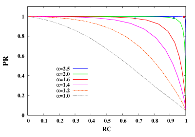
Let us take as a toy example the case of a sparse teacher with only $n_{\mbox{\tiny eff}}^{0}=5\%$ non-zero couplings. We set the noise to $\gamma=0$, such that there is always a perfect student solution. In particular, we will use a discrete teacher $J^{0}\in\{-1,0,1\}$

$$\rho(J^{0})=(1-0.05)\delta_{J^{0}}+\frac{0.05}{2}\left(\delta_{J^{0},-1}+\delta_{J^{0},1}\right)$$ (14)

With such a simple structure it happens to be the case that teacher’s dilution and variance are both equal $n_{\mbox{\tiny eff}}^{0}=t=0.05$.

The solution of the fixed point equations ((9) and (12)) is found numerically for different values of the amount of training data $\alpha$. For each $\alpha$, the different PR-RC curves are shown in Figure 1. It is clear from the figure that for sufficiently large $\alpha$, for instance $\alpha\geq 2.0$ in this example, the generalization is capable of a good classification of the couplings $J$, achieving both high precision and high recall, i.e. a good performance in model selection. This is seen in the figure as a curve that approaches the $PR\equiv 1$ line.

Figure 2: The statistical distribution of the students couplings $J$ for three different values of $\alpha$. When enough training data is given ($\alpha=2.5$ in this figure), the distribution $P(J)$ can be recognized as the superposition of Gaussian distributions located around the discrete (and rescaled) values of the teacher’s couplings. In such a case, setting to $0$ all those student’s couplings $J_{i}$ that are around $0$ results in a nearly perfect model reconstruction. As less information is used for training, the Gaussians overlap, and any threshold for the relevance of a coupling $J_{th}$ will misclassify some couplings, resulting in a worse model selection.

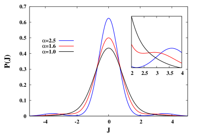
It is no surprise that more training data results in better model selection. However, we can gain some information about how the solution approaches perfect model selection by looking at the statistical distributions of the student’s $J$s. Figure 2 shows how $P(J)=\int\mathrm{d}J^{0}P(J^{0},J)$ (Eq. (13)) concentrates around the discrete (and rescaled) values of $J^{0}$ with a set of Gaussians that have neglectable overlap for large values of $\alpha$. Above a critical $\alpha\simeq 1.6$ (in this example) we can start to discriminate the $J$s from different Gaussians because local minima in $P(J)$ emerge. It is expected that above this point a reasonable value for $J_{th}$ is the one satisfying

$$\frac{\partial P(J)}{\partial J}=0\quad\frac{\partial^{2}P(J)}{\partial J^{2}}>0\ .$$

This choice for $J_{th}$ leads to the recall and precision, which can be seen in Figure 1 marked by the square symbols. For $\alpha=2.5$ the Gaussians in $P(J)$ are almost perfectly distinguishable. The optimal choice for $J_{th}$ has a precision and a recall near one $(RC\cong 0.991,PR\cong 0.996)$, meaning that generalization is achieving an almost perfect model selection.

IV Diluted generalization

At zero temperature (infinite $\beta$) and $h=0$, the Gibbs measure gives the same probability to all perfect student solutions, since they have the same energy $E(\vec{J})=0$, while suppressing completely positive-cost students. Working at zero temperature, a dilution field $h>0$ gives the chance to impose a different measure over the set of perfect solutions. This measure favors the students with the lowest values of $\|\vec{J}\|_{p}$, and in the limit of $h\to\infty$, it concentrates in the perfect solution with the highest $\mbox{L}_{p}$ dilution. We will now study the properties of the subset of perfect students with the smallest $\mbox{L}_{p}$ norm.

Unlike the trivial $\beta\rightarrow\infty$ limit (see Eq. (7)), the large-dilution limit has to be taken carefully as some parameters diverge. For large dilution field $h\to\infty$ we have $q\rightarrow 1$, meaning that different students are very close to each other, and in the limit $h=\infty$ there is only one student which is at the same time zero-cost ($E(\vec{J})=0$) and maximally diluted. As can be seen from the fixed point equations (9), when $q$ tends to 1, the order parameters $\hat{q}$, $\hat{r}$ and $\lambda$ diverge. The scaling behavior of these variables is the following

$$\begin{array}[]{rcllrcl}(1-q)&\simeq&\frac{Q}{h}&&\hat{r}&\simeq&\hat{R}h\\ \hat{q}&\simeq&\hat{Q}h^{2}&&\frac{\hat{q}}{2}-\lambda&\simeq&\frac{K}{2}h\end{array}$$ (15)

In terms of these new variables, the fixed point equations for $\hat{q}$ and $\hat{r}$ (9) become

$$\hat{Q} = \frac{\alpha}{\pi Q^{2}}\left[\mbox{ArcCot}\frac{r}{\sqrt{\gamma^{2}+t-r^{2}}}-\frac{r\sqrt{\gamma^{2}+t-r^{2}}}{\gamma^{2}+t}\right]$$

$$\hat{R} = \frac{\alpha\sqrt{\gamma^{2}+t-r^{2}}}{Q\pi(\gamma^{2}+t)}$$ (16)

and do not depend on the dilution $p$. Furthermore, this scaling makes the exponent of the exponential term inside $P[x,J^{0},J]$ (Eq. (8)) proportional to $h$. So, in the remaining three equations

$$Q = \frac{1}{\sqrt{\hat{Q}}}\mathbf{E}[xJ]$$

$$r = \mathbf{E}[J^{0}J]$$ (17)

$$1 = \mathbf{E}[J^{2}]$$

the expectation values for $h\to\infty$ are dominated by the largest values of the exponent in (8). The specific details of this saddle-point calculation depend on the actual dilution $\|\vec{J}\|_{p}$.

Among all possible values of $p$, the cases $p=1$ and $p=0$ are special for both their meaning and their simplicity in the calculations. The $\mbox{L}_{1}$ norm is extremely popular in machine learning because it maintains the convexity of a convex cost function while forcing sparse solutions Tibshirani (1994). On the other hand, $\mbox{L}_{0}$ lacks completely of the convexity preserving property (it is not even continuous), and therefore is not a suitable penalization for convex optimization. However, the $\mbox{L}_{0}$ norm is optimal in the sense that it does not deform the Hamiltonian beyond penalizing non-zero couplings. We will compare the dilution achieved by the $\mbox{L}_{1}$ approach with the largest possible dilution (the one obtained using $\mbox{L}_{0}$ ), and give a qualitative description of this widely used regularization. Another simple and common choice for the penalization is $p=2$, but in our model setting it is meaningless since the student is constrained to the sphere and therefore has a fixed $\|\vec{J}\|_{2}=N$.

IV.1 $\mbox{L}_{1}$ dilution

We first discuss the case of $\mbox{L}_{1}$ -regularization $\|\vec{J}\|_{1}=\sum_{i=1}^{N}|J_{i}|$. For $h\to\infty$ the expectation value of an arbitrary function $g(x,J^{0},J)$ is given by

$$\mathbf{E}[g(x,J^{0},J)]=\int\mathrm{D}x\>\int\mathrm{d}J^{0}\rho(J^{0})\times\left\{\begin{array}[]{lll}g(x,J^{0},0)&&|\hat{R}J^{0}-\sqrt{\hat{Q}}x|<1\\ g(x,J^{0},\frac{\hat{R}J^{0}-\sqrt{\hat{Q}}x-\mathrm{Sign}(\hat{R}J^{0}-\sqrt{\hat{Q}}x)}{K})&&\mbox{ otherwise.}\end{array}\right.$$

The derivation of this expectation value is shown in appendix B. As already mentioned, one of the virtues of the $\mbox{L}_{1}$ -regularization is that it forces the solution to be diluted by setting a fraction of the couplings exactly to zero. This fact becomes evident in the previous equation.

Using the scaling behavior (15), and calling $S(J^{0},x)=\mathrm{Sign}(\hat{R}J^{0}-\sqrt{\hat{Q}}x)$, and defining the functional

$$L[\cdot]=\int\mathrm{D}x\>[\cdot]\Theta(|\hat{R}J^{0}-\sqrt{\hat{Q}}x|-1)\>\mbox{,}$$

the resulting fixed-point equations in the $h\to\infty$ limit are (16) and

$$Q = \frac{1}{K}\int\mathrm{d}J^{0}\rho(J^{0})L[1]$$ (18)

$$r = \frac{1}{K}\int\mathrm{d}J^{0}\rho(J^{0})\left[\hat{R}{J^{0}}^{2}L[1]-\sqrt{\hat{Q}}J^{0}L[x]-J^{0}L[S(J^{0},x)]\right]$$

$$K = (\hat{Q}+1)Q+r\hat{R}+\frac{1}{K}\int\mathrm{d}J^{0}\rho(J^{0})\left[\sqrt{\hat{Q}}L[xS(J^{0},x)]-\hat{R}J^{0}L[S(J^{0},x)]\right]$$

Note that the original parameter $q$ is no longer present, since it is $1$, but the overlap between teacher and student, $r$, is still a non trivial order parameter.

IV.2 $\mbox{L}_{0}$ dilution

For the $\mbox{L}_{0}$ -regularization the dilution term in the Hamiltonian (3) is $\|\vec{J}\|_{0}=\sum_{i}^{N}(1-\delta_{J_{i}})$, punishing only the fact that a given $J_{i}$ is non zero, but otherwise making no distinction between different non-zero $J$-values. In a strict mathematical sense, introducing the $\mbox{L}_{0}$ norm in the Hamiltonian is meaningless, since a finite single-point discontinuity cannot alter the integration over the continuous range of $J$-values in the partition function. So the $\mbox{L}_{0}$ norm can only be understood as the limiting case $p\to+0$ of a family of continuous functions (see appendix C).

Using a similar approach as the one presented in appendix B for $\mbox{L}_{1}$ , the expectation value of an arbitrary function $g(x,J^{0},J)$ in the $h\to\infty$ limit reads

$$\mathbf{E}[g(x,J^{0},J)]=\int\mathrm{D}x\>\int\mathrm{d}J^{0}\rho(J^{0})\left\{\begin{array}[]{lll}g(x,J^{0},0)&&\frac{|\hat{R}J^{0}-\sqrt{\hat{Q}}x|}{\sqrt{2K}}<1\\ g(x,J^{0},\frac{\hat{R}J^{0}-\sqrt{\hat{Q}}x}{K})&&\mbox{ otherwise}\end{array}\right.$$ (19)

The fixed-point equations for $\hat{Q}$ and $\hat{R}$ are exactly the same as for $\mbox{L}_{1}$ -dilution (eq. (16)), while the other three order parameters are now given by

$$Q = \frac{1}{K}\int\mathrm{d}J^{0}\rho(J^{0})\left[M[1]-\frac{1}{\sqrt{\hat{Q}}}\tilde{M}[xS(J^{0},x)]\right]$$

$$r = \frac{1}{K}\int\mathrm{d}J^{0}\rho(J^{0})\left[\hat{R}{J^{0}}^{2}M[1]-\sqrt{\hat{Q}}J^{0}M[x]\right]$$ (20)

$$K = r\hat{R}+Q\hat{Q}$$

where $M[\cdot]=\int\mathrm{D}x\>\>[\cdot]\>\theta(\frac{|\hat{R}J^{0}-\sqrt{\hat{Q}}x|}{\sqrt{2K}}-1)$, and $\tilde{M}[xS(J^{0},x)]$ is defined as

$$\tilde{M}[xS(J^{0},x)]=-\frac{2\sqrt{2K}}{\sqrt{2\pi}}\exp{-\frac{\hat{R}^{2}{J^{0}}^{2}+2K}{2\hat{Q}}}\cosh{\frac{\hat{R}J^{0}\sqrt{2K}}{\hat{Q}}}\ .$$

IV.3 Dilution, recall and precision

The numerical solution of the fixed-point equations for the $\mbox{L}_{1}$ and $\mbox{L}_{0}$ dilutions gives us the overlap $r$ between the teacher and the student. The generalization error is obtained using Eq. (10).

The most striking effect of the norms is the emergence of an extensive number of couplings that are exactly zero (see $P(J)$ in appendices). The fraction of non-zero couplings is the effective dilution $n_{\mbox{\tiny eff}}$ achieved by the student, and it is obtained as

$$n_{\mbox{\tiny eff}}\>=\mathbf{E}[|J|>0]=\left\{\begin{array}[]{llll}\int\mathrm{d}J^{0}\rho(J^{0})L[1]\>=QK&\>\>\>L_{1}\mbox{ norm}\\ \int\mathrm{d}J^{0}\rho(J^{0})M[1]&\>\>\>L_{0}\mbox{ norm}\end{array}\right.$$ (21)

It is expected (and numerically observed) that for large values of $\alpha$ the effective dilution $n_{\mbox{\tiny eff}}$ converges to the real dilution of the teacher $n_{\mbox{\tiny eff}}^{0}$.

Along the same lines developed for the non-diluted case, we can further restrict the set of non-zero couplings by setting a threshold for relevant couplings. In other words, we interpret as non-relevant all those couplings that are not strong enough, $J_{i}<|J_{th}|$. In this case, the fraction of relevant couplings equals

$$n_{\mbox{\tiny eff}}^{th}\>=\mathbf{E}[\Theta(|J|-J_{th})]$$

and can be used to calculate the precision according to Eq. (11). The other terms appearing in recall and precision are also computed using the expectation value $\mathbf{E}[\cdot]$ for each dilution scheme. For instance, the probability of having a false positive is given by $P_{FP}=\mathbf{E}[\Theta(|J|-J_{th})\delta_{J^{0}}]$.

V How well does dilution work?

The discussed mathematical machinery can shed some light on this question. To see the differences between diluted and non-diluted generalization, and its performance in sparse model selection, let us use the same toy example used for the non-diluted case, with a teacher of dilution $n_{\mbox{\tiny eff}}^{0}=5\%$ and discrete values $J_{i}^{0}\in\{-1,0,1\}$, see Eq. (14).

Figure 3: The dilution $n_{\mbox{\tiny eff}}(\alpha)$ achieved by the $\mbox{L}_{1}$ and $\mbox{L}_{0}$ dilutions, as a function of the amount of training patterns $\alpha$. The $\mbox{L}_{0}$ regularization approaches the dilution of the teacher $n_{\mbox{\tiny eff}}^{0}=0.05$ from below, including non zero couplings only when strictly required to correctly classify the training data. The $\mbox{L}_{1}$ dilution is not that efficient, and for $\alpha>0.45$ it uses more non-zero couplings than actually needed.

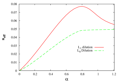
The functions $n_{\mbox{\tiny eff}}(\alpha)$ for the $\mbox{L}_{1}$ and $\mbox{L}_{0}$ dilutions are presented in Fig. 3. It can be seen that $\mbox{L}_{0}$ -diluted generalization goes monotonously from below to the correct value $n_{\mbox{\tiny eff}}=0.05$, in a somehow Ocams-optimal way. In other words, $\mbox{L}_{0}$ dilution adds non-zero couplings just when strictly required by the empirical (training) evidence. The $\mbox{L}_{1}$ norm isn’t that effective. It is an interesting result that, for a certain range in $\alpha$, the $\mbox{L}_{1}$ optimal solution requires more non-zero couplings ($n_{\mbox{\tiny eff}}>n_{\mbox{\tiny eff}}^{0}=0.05$) than actually present in the teacher. This overshooting is the cost we pay for deforming the Hamiltonian by the $\mbox{L}_{1}$ -penalization of large couplings. Unlike $\mbox{L}_{0}$ regularization, $\mbox{L}_{1}$ approaches the correct dilution from above, not from below.

Figure 4: The generalization error at different $\alpha$. The two curves at the center are the generalization error achieved using $\mbox{L}_{1}$ and $\mbox{L}_{0}$ dilution. While the $\mbox{L}_{1}$ error decreases smoothly with the training data, the one corresponding to $\mbox{L}_{0}$ undergoes a sudden drop near $\alpha=0.8$. This is a consequence of a sudden move to almost perfect model selection, where the set of non-zero interactions has been identified with very good precision. Both, the superior and lower curves, correspond to the non-diluted generalization, where the lower one has been plotted with rescaled $x$-axis, $\epsilon(\alpha/n_{\mbox{\tiny eff}}^{0})$. If the student could know from the beginning which are the non-zero couplings, it could use all the training data to tune the values of these couplings, resulting in a huge reduction of the generalization error.

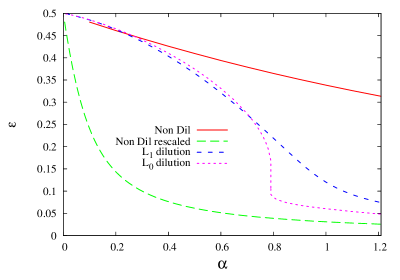
One could be tempted to call the change of slope of $\mbox{L}_{0}$ near $\alpha=0.8$ in Fig. 3 a transition to perfect student solution, but it is not. The generalization error in Fig. 4 shows that errors persist also for larger $\alpha$. On the other hand, while the $\mbox{L}_{1}$ norm goes smoothly to $\epsilon=0$, the $\mbox{L}_{0}$ undergoes an abrupt reduction of the generalization error near $\alpha=0.8$. This might be a sign of a transition to (almost) perfect model selection, such that for $\alpha>0.8$ the student has identified the correct $J_{i}=0$, and its mistakes are restricted to the actual values of those $J_{i}$s that are non-zero.

Figure 5: The PR-RC curves of the non-diluted, $\mbox{L}_{1}$ diluted, and $\mbox{L}_{0}$ diluted generalization for four different values of $\alpha$. Both, the $\mbox{L}_{1}$ and $\mbox{L}_{0}$ dilutions, outperform the non-diluted generalization. Particularly, the $\mbox{L}_{0}$ dilution moves suddenly to almost perfect model selection near $\alpha=0.8$.

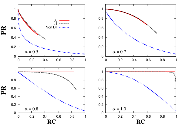
To compare the $\mbox{L}_{1}$ and $\mbox{L}_{0}$ dilutions to non-diluted generalization, we show the PR-RC curves in Fig. 5, for four typical values of $\alpha$. The curves for the diluted generalization seem to miss the right part – but they are not. As the $\mbox{L}_{1}$ and $\mbox{L}_{0}$ methods set a fraction of the couplings exactly to zero, lowering the threshold $J_{th}$ will never achieve to include them as non-zero couplings, and this is why we can not arrive at recall equal to one.

Looking to the PR-RC curves, the first obvious fact is that the non-diluted generalization is much worse than any of the diluted ones. The next interesting fact is that $\mbox{L}_{1}$ performs slightly better than $\mbox{L}_{0}$ for low values of $\alpha$, something that could be seen also from the generalization error (Fig. 4). Finally the sudden change to $PR\cong 1$, for $\alpha=0.8$, of the PR-RC curve for the $\mbox{L}_{0}$ dilution is saying that $\mbox{L}_{0}$ fastly moves to almost perfect model selection, as we guessed from the generalization error curve. However, there is no critical $\alpha$, and the sudden change is not a phase transition. This can be seen more clearly working with less diluted teachers (for instance $n_{\mbox{\tiny eff}}^{0}=0.1$, data not shown). To gain some more understanding of the onset of an almost perfect model selection it is interesting to see the distribution of couplings, $P(J)$, which are shown in appendices B and C.

VI The memorization limit

In the calculations presented so far, the noise $\eta^{\mu}$ affecting the output $y^{\mu}$ in Eq. (2), was neglected by setting its variance to $\gamma^{2}=0$. By doing so, we guaranteed that for any $\alpha$, there is always at least one zero-cost solution for the student, namely $\vec{J}=\vec{J^{0}}$. Let us now study the opposite extreme case where the noise is extremely large. In that case, the output function is given by

$$y^{\mu}=\sigma^{0}(\vec{x})=\mathrm{Sign}(\eta^{\mu})\ ,$$

i.e. the patterns are randomly classified by $y^{\mu}=\pm 1$. The teacher’s couplings $J_{i}^{0}$ become irrelevant, and the student will try to learn (generalize) a non-existing hidden relation. This limit is equivalent to the well-studied memorization problem of random input-output relation. It is a classical result Gardner (1988) that for $\alpha>2$ the student will fail to correctly classify all patterns, while for $\alpha<2$ the student can find a solution of zero energy. In the latter case, the student vector $\vec{J}$ reproduces correctly the relation between the $M$ patterns $\vec{x}^{\mu}$ and the corresponding labels $y^{\mu}$ by $y^{\mu}=\mathrm{Sign}(\vec{J}\cdot\vec{x}^{\mu})$. The student was capable of memorizing the labeling of the input patterns.

Therefore memorization can be studied as the noise-dominated limit of generalization. By computing the limit $\gamma\to\infty$ in the fixed point equations for $\hat{q}$ and $\hat{r}$ (9), we found that $\hat{r}=0$ while

$$\hat{q}=\frac{\alpha}{\sqrt{2\pi q(1-q)}}\int\mathrm{D}x\>\frac{x}{H(\sqrt{q}x)}$$ (22)

The expectation value of a function $g(x,J)$ becomes

$$\mathbf{E}[g(x,J)]=\int\mathrm{D}x\>\frac{\int\mathrm{d}J\>g(x,J)e^{-(\frac{\hat{q}}{2}-\lambda)J^{2}-h\|J\|_{p}-\sqrt{\hat{q}}x)J}}{\int\mathrm{d}Je^{-(\frac{\hat{q}}{2}-\lambda)J^{2}-h\|J\|_{p}-\sqrt{\hat{q}}x)J}}$$ (23)

In particular we have $r=\mathbf{E}[J^{0}J]=0$, meaning that the overlap between student and teacher is zero, which is an obvious consequence of the large-noise limit. So, the set of variational parameters describing our problem reduces to $q,\hat{q}$ and $\lambda$, and the fixed-point equations are (22) and

$$q=1+\frac{1}{\sqrt{\hat{q}}}\mathbf{E}[xJ]\qquad 1=\mathbf{E}[J^{2}]\ .$$

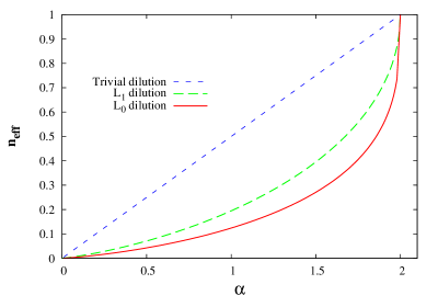
The generalization error and the precision-vs.-recall curve are meaningless in this context. However, we can still check the efficiency of the $\mbox{L}_{1}$ and $\mbox{L}_{0}$ memorizations in using as few as possible non-zero couplings to memorize a set of patterns. There is a first trivial conclusion, coming from the already stated fact that a continuous perceptron is capable of memorizing without error until $\alpha=2$. This means that a perceptron with $N$ couplings $J_{i}$ can remember the classification of $M=2N$ patterns. It follows directly from this that if $\alpha<2$ patterns are given, we can set to zero any fraction $1-\alpha/2$ of the couplings, and still be capable of memorizing without error with the remaining $\alpha/2$ couplings. We are interested in how much more dilution can be obtained by the introduction of a dilution term in the Hamiltonian. Note that if, instead of setting to zero a random group of $(1-\alpha/2)N$ couplings, we optimize their selection, we can go far below the trivial $n_{\mbox{\tiny eff}}=\alpha/2$ dilution.

Figure 6: The maximum dilution achieved when using the $\mbox{L}_{1}$ and $\mbox{L}_{0}$ regularizations in the Memorization problem. The trivial dilution $n_{\mbox{\tiny eff}}=\alpha/2$ is outperformed by either $\mbox{L}_{0}$ and $\mbox{L}_{1}$ dilutions, and $\mbox{L}_{0}$ is the more efficient of all. For $\alpha>2$ the student fails to memorize all patterns and there is no student solution of zero energy.

We can solve the fixed-point equations in the limit of large dilution fields $h\to\infty$. Once again the solution space reduces to only one solution $q\to 1$, so there are some divergences in the equations. The scaling behavior of the variational parameters is the following

$$(1-q) \simeq \frac{Q}{h}$$

$$\hat{q} \simeq \hat{Q}h^{2}$$

$$\frac{\hat{q}}{2}-\lambda \simeq \frac{K}{2}h$$

Using this scaling, the expectation values are given by

$$\mathbf{E}[g(x,J)]=\int\mathrm{D}x\>\left\{\begin{array}[]{lll}g(x,0)&&x^{2}<\frac{1}{\hat{Q}}\\ g(x,\frac{\sqrt{\hat{Q}}x-\mathrm{Sign}(x)}{K})&&\mbox{ otherwise}\end{array}\right.$$

for the $\mbox{L}_{1}$ case, and

$$\mathbf{E}[g(x,J)]=\int\mathrm{D}x\>\left\{\begin{array}[]{lll}g(x,0)&&x^{2}<\frac{2K}{\hat{Q}}\\ g(x,\frac{\sqrt{\hat{Q}}x}{K})&&\mbox{ otherwise}\end{array}\right.$$

for the $\mbox{L}_{0}$ case.

Solving numerically the corresponding fixed point equations, we can compute the dilution achieved by each method

$$n_{\mbox{eff}} = 1-D[\delta_{J,0}]=\left\{\begin{array}[]{ll}2H\left(\hat{Q}^{-1/2}\right)&\qquad\mbox{L}_{1}\>\mbox{Norm}\\ 2H\left(\sqrt{2K}\hat{Q}^{-1/2}\right)&\qquad\mbox{L}_{0}\>\mbox{Norm}\end{array}\right.$$

The resulting functions $n_{\mbox{\tiny eff}}(\alpha)$ are show in Figure 6. It shows that both $\mbox{L}_{1}$ and $\mbox{L}_{0}$ achieve a much stronger dilution than the trivial random one. As in the generalization case, the $\mbox{L}_{1}$ regularization works worse than $\mbox{L}_{0}$ , the reason being that it penalizes large $J$ values. The dilution achieved in memorization for the $\mbox{L}_{1}$ and $\mbox{L}_{0}$ dilutions is always above the corresponding generalization curves in Fig. 3. Although not shown in either figures, we checked that near $\alpha=0$ the corresponding curves coincide, as there is no difference between learning and memorizing when too few training data are given.

VII Conclusions

In this paper, we have presented an analytical replica computation on the generalization properties of a sparse continuous perceptron. Dilution has been achieved in different ways: First, it can be imposed naively by using non-diluted inference, followed by deleting all those couplings which are below some threshold value. Second, it can be achieved by introducing a dilution field which is coupled to the $L_{p}$-norm of the coupling vector, penalizing thereby vectors of high norm. For $p\leq 1$, the cusp-like singularity of the $L_{p}$-norm in zero forces a finite fraction of all couplings to be exactly zero. We have studied in particular two special cases: (i) $p=1$ is a popular choice in convex optimization since it is the only value of $p$ which corresponds both to a convex penalty function and dilution. (ii) $p=0$ achieves optimal dilution since it penalizes equally all non-zero couplings independently on their actual value, but due to the non-convex character of this penalty, it easily leads to computational intractability.

As a first finding, we see that both $L_{p}$ schemes work fundamentally better than the naive scheme, both in the questions of model selection (i.e. for the identification of topological properties of the data-generating perceptron given by its non-zero couplings) and in the generalization ability. For a very small or a very large amount of training data, $L_{0}$ and $L_{1}$ achieve very comparable results. We find, however, an intermediate regime where $L_{0}$ suddenly improves its performance toward almost perfectly model selection, whereas $L_{1}$ dilution shows a more gradual increase in performance. This is very interesting since this regime is found for relatively small data sets, and in many current inference tasks (e.g. in computational biology) the quantity of data is the major limiting factor for the computational extraction of information. It might be in this parameter region, where statistical-physics based algorithms like the ones presented in Kabashima (2003); Uda and Kabashima (2005); Kabashima (2008); Braunstein et al. (2008a, b); Pagnani et al. (2009) may outperform methods based on convex optimization proposed in Tibshirani (1994).

These analytic results call for efficient algorithms in real case studies. At odds with the linear-regression case with $\mbox{L}_{1}$ norm, in the case of a continuous perceptron, a simple gradient descent strategy does not work due to the presence of a zero-mode in the energetic term Eq. (1) ($E(\vec{J})=E(c\vec{J})$ for every scalar $c>0$). The zero-mode has been removed in the computation by fixing the modulus of the classification vector ($\vec{J}\cdot\vec{J}=N$). Unfortunately this spherical constraint breaks the convexity of the problem and it is not clear if there are more ingenious ways for removing the zero-mode that could work, at least in the $\mbox{L}_{1}$ norm case. Another possibility that we are planning to follow is that of considering variational approximation schemes like belief propagation for continuous perceptrons Kabashima (2008); Braunstein et al. (2008b); Pagnani et al. (2009), which are able to overcome also the problem of the non-convexity of the $L_{0}$ norm.

During the preparation of this manuscript, a related study on the efficiency of $\mbox{L}_{p}$ dilution in systems of linear equations was posted online Kabashima et al. . Also there, the relative importance of $L_{0}$ and $L_{1}$ dilution was studied, with conclusions which are highly compatible to ours.

Appendix A Replica calculation details

The calculation of $\overline{Z^{n}}$ in Eq. (II.1) is done by the introduction of an overlap matrix $Q_{a,b}$ using constraints

$$\delta(NQ_{a,b}-\sum_{i}J_{i}^{a}J_{i}^{b})$$

for any $0\leq a\leq b\leq n$. As there is a symmetry in the replica indices $Q_{a,b}=Q_{b,a}$, only the half of the matrix is needed. The value $a=0$ refers to the teacher, while $a=1\ldots n$ to the $n$-fold replicated student. Among these constraints, there are some that are particular. For instance the term $Q_{0,0}$ is the variance of the teacher, and it should be equal to the variance $t$ of the teachers distribution (4). Similarly, the $n$ terms $Q_{a,a}$ are set to $1$, in order to impose the spherical constraint on the student, since the energy (1) is invariant to elongations of the student vector.

Using Fourier representation of the Dirac-deltas, the replicated partition function is

$$\overline{Z^{n}}=\int\frac{\mathrm{d}Q_{a,b}\mathrm{d}\hat{Q}_{a,b}\mathrm{d}^{n}\lambda^{a}}{(2\pi)^{3/2}N^{-1}}\exp\left(iN\sum_{a<b}Q_{a,b}\hat{Q}_{a,b}+iN\sum_{a>0}\lambda_{a}+iNt\lambda_{0}\right)$$

$$\left(\int\mathrm{d}^{n}J^{a}\rho(J^{0})\exp(-h\sum_{a}^{n}\|J^{a}\|_{p}-i\sum_{a\leq b}J^{a}\hat{Q}_{a,b}J^{b})\right)^{N}$$ (25)

$$\left(\int\mathrm{D_{\gamma}}\eta\frac{\mathrm{d}^{n}X^{a}\mathrm{d}^{n}\hat{X}^{a}}{2\pi}\exp(-\beta\sum_{a}^{n}\theta\left(-(X^{0}+\eta)X^{a}\right)+i\sum_{a}X^{a}\hat{X}^{a}-\frac{1}{2}\sum_{a,b}\hat{X}^{a}Q_{a,b}\hat{X}^{b})\right)^{M}$$

where $\hat{Q}_{a,b}$ are the conjugated parameters in the Fourier representation of the deltas. In particular, $\lambda^{0}$ and $\lambda^{a}$ are the one corresponding to the teacher variance and the spherical constraint. To save some space, we used the short-hand notation $\mathrm{d}^{n}A^{a}$ as a substitute for $\prod_{a=0}^{n}\mathrm{d}A^{a}$, and $\mathrm{d}Q_{a,b}$ for the differential of all the terms in the overlap matrix.

The next step in the replica calculation is to assume a structure for the overlap matrix. In the replica-symmetric case, the overlap matrix and its Fourier counterpart have the structure (exemplified for $n=3$)

$$Q_{a,b}=\left(\begin{array}[]{cccc}t&&&\\ r&1&&\\ r&q&1&\\ r&q&q&1\end{array}\right)\quad-i\hat{Q}_{a,b}=\left(\begin{array}[]{cccc}\lambda^{0}&&&\\ \hat{r}&\lambda&&\\ \hat{r}&\hat{q}&\lambda&\\ \hat{r}&\hat{q}&\hat{q}&\lambda\end{array}\right)$$ (26)

The Fourier mode corresponding to the variance of the teacher $t$, can be shown to be $\lambda^{0}=0$, while that of the spherical constraint remains a variational parameter $\lambda=-i\lambda^{a}$. The other parameters are $q$, the self overlap between two student solutions, $r$, the overlap between an student and the teacher, and their conjugate Fourier modes $\hat{q}$ and $\hat{r}$.

It is a standard feature of the replica trick to invert the order of the limits, doing $N\rightarrow\infty$ first, and then $n\rightarrow 0$, profiting thereby of the saddle-point method to solve the integral in (25). Note that the last two lines in (25) can be brought to the exponential by using $X=\exp\log X$. Thus the value of the free energy $-\beta\overline{f}=\lim_{n\to 0}\lim_{N\to\infty}\frac{1}{Nn}\log\overline{Z^{n}}$ is given by extremizing the equation

$$-\beta\overline{f}=-r\hat{r}+\frac{1}{2}q\hat{q}-\lambda+G_{J}+\alpha\>G_{X}$$

with respect to the variational parameters $(q,r,\hat{q},\hat{r},\lambda)$, where we have introduced

$$G_{J} = \int\mathrm{D}x\>\int\mathrm{d}J^{0}\rho(J^{0})\log\int\mathrm{d}Je^{-(\frac{\hat{q}}{2}-\lambda)J^{2}-h\|J\|_{p}+(\hat{r}J^{0}-\sqrt{\hat{q}}x)J}$$

$$G_{X} = 2\int\mathrm{D}x\>H\left(\frac{xr}{\sqrt{q\gamma^{2}+qt-r^{2})}}\right)\log\left((e^{-\beta}-1)H(-\sqrt{\frac{q}{1-q}}x)+1\right)$$

and

$$H(x)=\int_{x}^{\infty}\frac{\mathrm{d}y}{\sqrt{2\pi}}e^{-y^{2}/2}$$

Appendix B Limit $h\rightarrow\infty$

The scaling behavior of the parameters $q,r,\hat{q},\hat{r}$ and $\lambda$ in the limit $h\to\infty$

$$\begin{array}[]{rcllrcl}(1-q)&\simeq&\frac{Q}{h}&&\hat{r}&\simeq&\hat{R}h\\ \hat{q}&\simeq&\hat{Q}h^{2}&&\frac{\hat{q}}{2}-\lambda&\simeq&\frac{K}{2}h\end{array}$$

were first obtained by looking at the solutions of the fixed-point equations for growing values of $h$, and their consistency was checked later in the fixed-point equations. Considering this scaling, the expectation value of a generic function $g(x,J^{0},J)$ is given by

$$\mathbf{E}[g(x,J^{0},J)]=\int\mathrm{D}x\>\mathrm{d}J^{0}\rho(J^{0})\frac{\int\mathrm{d}J\>g(x,J^{0},J)e^{-h\left(\frac{K}{2}J^{2}+\|J\|_{p}-(\hat{R}J^{0}-\sqrt{\hat{Q}}x)J\right)}}{\int\mathrm{d}Je^{-h\left(\frac{K}{2}J^{2}+\|J\|_{p}-(\hat{R}J^{0}-\sqrt{\hat{Q}}x)J\right)}}$$ (27)

The diverging prefactor $h$ in the exponentials forces the main contribution to the $J$-integration to come from the largest value of the exponent (saddle-point approximation):

$$J^{*}_{p}=\mathop{{\mbox{argmin}}\vphantom{\sim}}\limits_{{}_{\mathbf{J}}}\left(\frac{K}{2}J^{2}+\|J\|_{p}-(\hat{R}J^{0}-\sqrt{\hat{Q}}x)J\right)$$ (28)

In the case of the $\mbox{L}_{1}$ norm ($\|J\|_{1}=|J|$) the solution of the previous equation is given by

$$J=\left\{\begin{array}[]{lll}0&&|\hat{R}J^{0}-\sqrt{\hat{Q}}x|<1\\ \frac{\hat{R}J^{0}-\sqrt{\hat{Q}}x-\mathrm{Sign}(\hat{R}J^{0}-\sqrt{\hat{Q}}x)}{K}&&\mbox{ otherwise}\end{array}\right.$$ (29)

The expectation value is thus

$$\mathbf{E}[g(x,J^{0},J)]=\int\mathrm{D}x\>\int\mathrm{d}J^{0}\rho(J^{0})\left\{\begin{array}[]{lll}g(x,J^{0},0)&&|\hat{R}J^{0}-\sqrt{\hat{Q}}x|<1\\ g(x,J^{0},\frac{\hat{R}J^{0}-\sqrt{\hat{Q}}x-\mathrm{Sign}(\hat{R}J^{0}-\sqrt{\hat{Q}}x)}{K})&&\mbox{ otherwise}\end{array}\right.$$

Figure 7: The distribution $P(J)$ of the student couplings for the four values of $\alpha$ used in the Precision-Recall curves of Fig. 5.

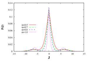
The probability distribution of the students couplings $P(J)$ can be obtained as $P(J^{\prime})=\mathbf{E}[\delta(J-J^{\prime})]$ resulting in

$$P(J)=(1-n_{\mbox{\tiny eff}})\>\delta(J)+\frac{K}{\sqrt{\hat{Q}}\sqrt{2\pi}}\int\mathrm{d}J^{0}\rho(J^{0})e^{-\frac{(\hat{R}J^{0}-\mathrm{Sign}J-KJ)^{2}}{2\hat{Q}}}$$

where $n_{\mbox{\tiny eff}}=1-\int\mathrm{D}x\>\int\mathrm{d}J^{0}\rho(J^{0})\Theta[|\hat{R}J^{0}-\sqrt{\hat{Q}}x|-1]$. The continuous part of this distribution is shown in Fig. 7 for the same four values of $\alpha$ for which the Precision-Recall curves were shown in Fig. 5. We can see that for growing values of $\alpha$, the distribution $P(J)$ is more concentrated around the discrete values of $J$, and the amount of couplings that are small but not zero, reduces continuously. This explains the high performance in model selection of the $\mbox{L}_{1}$ dilution for $\alpha>1.0$.

Note that the calculation of the smallest value of the exponent in (27) is particularly simple for $\mbox{L}_{0}$ and $\mbox{L}_{1}$ . Other values of $p$ may require a numerical solution. It is simple to see that in the $p>1$ case no dilution is obtained.

Appendix C $\mbox{L}_{0}$ as the $p\to 0$ limit

The $\mbox{L}_{0}$ dilution corresponds to a term $\sum_{i}(1-\delta_{J_{i}})$ in the Hamiltonian (3). However, the Kronecker delta is zero for all non-zero arguments, with an isolated and finite discontinuity in the origin. This single-point discontinuity is irrelevant in the integration over continuous $J$s in the partition function as well as in (27). Therefore using the $\mbox{L}_{0}$ dilution from the beginning gives the same results as the non-diluted case $h=0$. Nevertheless, we can still interpret the $\mbox{L}_{0}$ norm as the $p\to+0$ limit of the $\mbox{L}_{p}$ norm.

Figure 8: The $p=0$ and $p>0$ cases of the function $Y_{p}(J)=\frac{K}{2}J^{2}+\|J\|_{p}-(\hat{R}J^{0}-\sqrt{\hat{Q}}x)J$ in the two characteristic situations where $J^{*}_{p}=0$ and $J^{*}_{p}>0$. The closer $p$ to zero, the closer the function $Y_{p}(J)$ is to $J_{0}(J)$.

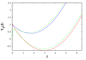
For general $p>0$ there is no explicit solution for Eq. (28). We will argue that the limit $p\to 0$ of such solutions is exactly the solution of

$$J^{*}_{0}=\mathop{{\mbox{argmin}}\vphantom{\sim}}\limits_{{}_{\mathbf{J}}}\left(\frac{K}{2}J^{2}+(1-\delta_{J})-(\hat{R}J^{0}-\sqrt{\hat{Q}}x)J\right)$$

just as if we would have introduced the $\mbox{L}_{0}$ norm from the beginning, and taken naively the saddle point including the isolated singularity. There are two candidate values for $J^{*}_{0}$, one is $0$ and the other one is the zero-derivative point of the quadratic function $J^{*}_{0}=\frac{\hat{R}J^{0}-\sqrt{\hat{Q}}}{T}$. The latter will be the actual solution if and only if

$$\frac{(\hat{R}J^{0}-\sqrt{\hat{Q}})^{2}}{2T}<1$$

If the opposite inequality is satisfied, the solution is $J^{*}_{0}=0$. Both situations are shown in Figure 8. The function $|J|^{p}$ tends to $1$ as $p\to 0$ for all $J\neq 0$, so we have also $J^{*}_{p}\to J^{*}_{0}$ whenever $\frac{(\hat{R}J^{0}-\sqrt{\hat{Q}})^{2}}{2T}\neq 1$. The point where the equality holds corresponds to the neglectable case when the value in $J=0$ is exactly equal to that in the point of zero derivative. We conclude that except for this single point, $J^{*}_{p}\to J^{*}_{0}$ as $p\to 0$, and therefore we can replace the $\mbox{L}_{0}$ norm directly into the steepest descend condition to obtain the $p\to 0$ result.

Figure 9: The distribution $P(J)$ of the student couplings for the four values of $\alpha$ used in the Precision-Recall curves of Fig. 5. Comparing also this result for $\mbox{L}_{0}$ with the one for $\mbox{L}_{1}$ in Fig. 7, we can understand the difference in their performance.

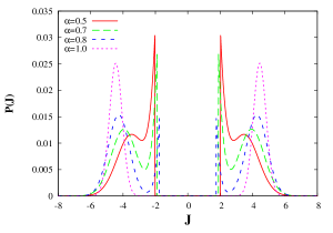
Repeating the steps shown in appendix B, a similar computation for the $\mbox{L}_{0}$ dilution gives the expectation value reported in Eq. (19), and the following probability distribution for the student couplings

$$P(J)=(1-n_{\mbox{\tiny eff}})\>\delta(J)+\frac{K}{\sqrt{\hat{Q}}\sqrt{2\pi}}\int\mathrm{d}J^{0}\rho(J^{0})e^{-\frac{(\hat{R}J^{0}-KJ)^{2}}{2\hat{Q}}}\Theta(|J|-\sqrt{\frac{2}{T}})$$

This distribution is shown in Fig. 9 for the same four values of $\alpha$ for which the Precision-Recall curves were shown in 5. Note that the main difference between this distribution and the corresponding to the $\mbox{L}_{1}$ dilution Fig. 7 is the presence of the $\Theta(\cdot)$ function in the former. When the Gaussians of the continuous part of the distribution have a standard deviation smaller than the gap in the $\Theta$ function, the presence of False Positives corresponding to the Gaussian around $J^{0}=0$ is suppressed by the $\Theta$ function, and this is the reason why we observe such a good performance in model selection for $\alpha>0.8$ in Fig. 5.

References

- Guyon and Elisseeff (2003) I. Guyon and A. Elisseeff, Journal of Machine Learning Research 3, 1157 (2003).
- Guyon et al. (2006) I. Guyon, S. Gunn, M. Nikravesh, and L. Zadeh, Feature Extraction: Foundations and Applications (Springer-Verlag, 2006).
- Tibshirani (1994) R. Tibshirani, Journal of the Royal Statistical Society, Series B 58, 267 (1994).
- Ravikumar et al. (2006) P. Ravikumar, M. Wainwright, and J. Lafferty, in Advances in Neural Information Processing Systems 19: Proc. 20th Annual Conf. (NIPS 2006) (MIT Press, 2006), pp. 1465–1472.
- Banerjee et al. (2006) O. Banerjee, L. El Ghaou, A. d’Aspremont, and G. Natsoulis, in ACM International Conference Proceeding Series (2006), vol. 148, pp. 12–18.
- Lee et al. (2007) S.-I. Lee, V. Ganapathi, and D. Koller, in Advances in Neural Information Processing Systems (NIPS 2006) (2007).
- Schmidt et al. (2007) M. Schmidt, A. Niculescu-Mizil, and K. Murphy, in Proc. 22nd AAAI Conf. on Artificial Intelligence (AAI) (2007).
- Meinshausen and Buehlmann (2006) N. Meinshausen and P. Buehlmann, Annal. Stat. 34 (2006).
- Malzahn (2000) D. Malzahn, Phys. Rev. E 61, 6261 (2000).
- Braunstein et al. (2008a) A. Braunstein, P. Pagnani, M. Weigt, and Z. R., J. Phys.: Conf. Ser. 95, 012016 (2008a).
- Braunstein et al. (2008b) A. Braunstein, A. Pagnani, M. Weigt, and R. Zecchina, Journal of Statistical Mechanics: Theory and Experiment 2008, P12001 (29pp) (2008b), URL http://stacks.iop.org/1742-5468/2008/P12001.
- Pagnani et al. (2009) A. Pagnani, F. Tria, and M. Weigt, Journal of Statistical Mechanics: Theory and Experiment 2009, P05001 (2009), URL http://stacks.iop.org/1742-5468/2009/P05001.
- Kabashima (2003) Y. Kabashima, J. Phys. A 36, 11111 (2003).
- Uda and Kabashima (2005) S. Uda and Y. Kabashima, J. Phys. Soc. Jpn. 74, 2233 (2005).
- Kabashima (2008) Y. Kabashima, Journal of Physics: Conference Series 95, 012001 (13pp) (2008), URL http://stacks.iop.org/1742-6596/95/012001.
- Gardner (1987) E. Gardner, Europhys. Lett. 4, 481 (1987).
- Gardner (1988) E. Gardner, Journal of Physics A: Mathematical and General 21, 257 (1988), URL http://stacks.iop.org/0305-4470/21/257.
- Györgyi (1990) G. Györgyi, Phys. Rev. Lett. 64, 2957 (1990).
- Seung et al. (1992) H. S. Seung, H. Sompolinsky, and N. Tishby, Phys. Rev. A 45, 6056 (1992).
- Engel and van den Broeck (2001) A. Engel and van den Broeck, Statistical mechanics of learning (Cambridge University Press, New York, 2001).
- Mézard et al. (1987) M. Mézard, G. Parisi, and M. Virasoro, Spin Glass Theory and Beyond (World Scientific, Singapore, 1987).
- (22) Y. Kabashima, T. Wadayama, and T. Tanaka, arXiv:0907.0914.