Learning Rates and States from Biophysical Time Series: A Bayesian Approach to Model Selection and Single-Molecule FRET Data

Abstract: Time series data provided by single-molecule Förster resonance energy transfer (smFRET) experiments offer the opportunity to infer not only model parameters describing molecular complexes, e.g. rate constants, but also information about the model itself, e.g. the number of conformational states. Resolving whether or how many of such states exist requires a careful approach to the problem of model selection, here meaning discriminating among models with differing numbers of states. The most straightforward approach to model selection generalizes the common idea of maximum likelihood — selecting the most likely parameter values — to maximum evidence: selecting the most likely model. In either case, such inference presents a tremendous computational challenge, which we here address by exploiting an approximation technique termed variational Bayes. We demonstrate how this technique can be applied to temporal data such as smFRET time series; show superior statistical consistency relative to the maximum likelihood approach; compare its performance on smFRET data generated from experiments on the ribosome; and illustrate how model selection in such probabilistic or generative modeling can facilitate analysis of closely related temporal data currently prevalent in biophysics. Source code used in this analysis, including a graphical user interface, is available open source via http://vbFRET.sourceforge.net.

Key words: FRET; smFRET; Hidden Markov Model (HMM); Model selection; Variational Bayes; statistical inference

1 Introduction

Single-molecule biology has triumphed at creating well-defined experiments to analyze the workings of biological materials, molecules, and enzymatic complexes. As the molecular machinery studied become more complex, so too do the biological questions asked and, necessarily, the statistical tools needed to answer these questions from the resulting experimental data. In a number of recent experiments, researchers have attempted to infer mechanical parameters (e.g., the typical step size of a motor protein), probabilistic parameters (e.g., the probability per turn that a topoisomerase releases from its DNA substrate), or kinetic parameters (e.g., the folding/unfolding rates of a ribozyme) via statistical inference (1, 2, 3, 4, 5, 6, 7, 8, 9). Often the question of interest is not only one of selecting model parameters but also selecting the model, including from among models which differ in the number of parameters to be inferred from experimental data. The most straightforward approach to model selection generalizes the common idea of maximum likelihood (ML) — selecting the most likely parameter values — to maximum evidence (ME): selecting the most likely model.

In this manuscript we focus on model selection in a specific example of such a biological challenge: revealing the number of enzymatic conformational states in single molecule FRET (smFRET) data. FRET (10, 11, 12, 13) refers to the transfer of energy from a donor fluorophore (which has been excited by short-wavelength light) to an acceptor fluorophore (which then emits light of a longer wavelength) with an efficiency which decreases as the distance between the fluorophores increases. The distance-dependence of the energy transfer efficiency implies that the quantification of the light emitted at both wavelengths from a fluorophore pair may be used as a proxy for the actual distance (typically $\sim$1–10 nm) between these fluorophores. Often a scalar summary statistic (e.g. the “FRET ratio” $I_{A}/(I_{A}+I_{D})$ of the acceptor intensity to the sum of the acceptor and donor intensities) is analyzed as a function of time, yielding time series data which are determined by the geometric relationship between the two fluorophores in a non-trivial way. When the donor and acceptor are biochemically attached to a single molecular complex, one may reasonably interpret such a time series as deriving from the underlying conformational dynamics of the complex.

If the complex of interest transitions from one locally stable conformation to another, the experiment is well modeled by a hidden Markov model (HMM) (14), a probabilistic model in which an observed time series (here, the FRET ratio) is conditionally dependent on a hidden, or unobserved, discrete state variable (here, the molecular conformation). HMMs have long been used in ion channel experiments in which the observed dynamic variable is voltage, and the hidden variable represents whether the channel is open or closed (15, 16). More recently, Talaga proposed adapting such modeling for FRET data (17), and Ha and coworkers developed HMM software designed for FRET analysis (18). Such existing software for biophysical time series analysis implement ML on individual traces and require users either to guess the number of states present in the data, or to overfit the data intentionally by asserting an excess number of states. Resulting errors commonly are then corrected via heuristics particular to each software package. It would be advantageous to avoid subjectivity (as well as extra effort) on the part of the experimentalist necessary in introducing thresholds or other parameterized penalties for complex models, as well as to derive principled approaches likely to generalize to new experimental contexts and data types. To that end, our aim here is to implement ME directly, avoiding overfitting even within the analysis of each individual trace rather than as a post-processing correction.

This manuscript begins by describing the general problem of using probabilistic or generative models for experimental data (generically denoted ${\bf{y}}$) in which one specifies the probability of the data given a set of parameters of biophysical interest (denoted ${\vec{\vartheta}}$) and possibly some hidden value of the state variable of interest (denoted ${\bf z}$). We then present one particular framework, variational Bayes, for estimating these parameters while at the same time finding the optimal number of values for the hidden state variable ${\bf z}$. (In this manuscript bold variables are reserved for those extensive in the number of observations.) We next validate the approach on synthetic data generated by an HMM, with parameters chosen to simulate data comparable to experimental smFRET data of interest. Having validated the technique, we apply it to experimental smFRET data and interpret our results. We close by highlighting advantages of the approach; suggesting related biophysical time series data which might be amenable to such analysis; and outlining promising avenues for future extension and developments of our analysis.

2 Parameter and model selection

Since the techniques we present here are natural generalizations of those which form the common introduction to statistical techniques in a broad variety of natural sciences, we first remind the reader of a few key ideas in inference necessary before narrowing to the description of smFRET data, briefly discussing ML methods for parameter inference and ME methods for model selection. Extensions to temporal biophysical data more generally will be discussed in Sec. 6. Note that, since the ML-ME discussion does not rely on whether or not the model features hidden variables, for the sake of simplicity we first describe in the context of models without hidden variables.

2.1 Maximum likelihood inference

The context in which most natural scientists encounter statistical inference is that of ML; in this problem setting, the model is specified by an expression for the likelihood $p({\bf{y}}|{\vec{\vartheta}})$ — i.e., the probability of the vector of data ${\bf{y}}$ given some unknown vector of parameters of interest ${\vec{\vartheta}}$. (While this is not often stated explicitly, this is the framework underlying minimization of $\chi^{2}$ or sums-of-squared errors; cf. Sec. A for a less cursory discussion.) In this context the ML estimate of the parameter ${\vec{\vartheta}}$ is

$${\vec{\vartheta}}_{*}=\operatornamewithlimits{argmax}_{\vec{\vartheta}}p({\bf{y}}|{\vec{\vartheta}}).$$ (1)

ML methods are useful for inference of parameter settings under a fixed model (or model complexity), e.g. a particular parameterized form with a fixed number of parameters. However, when one would like to compare competing models (in addition to estimating parameter settings), ML methods are generally inappropriate, as they tend to “overfit”, since likelihood increases monotonically with model complexity.

This problem is conceptually illustrated in the case of inference from FRET data as follows: if a particular system has a known number of conformational states, say $K=2$, one can estimate the parameters (the transition rates between states and relative occupation of states per unit time) by maximizing the likelihood, which gives a formal measure of the “goodness of fit” of the model to the data. Consider, however, an overly complex model for the same observed data with $K=3$ conformational states, which one might do if the number of states is itself unknown. The resulting parameter estimates will have a higher likelihood or “better” fit to the data under the maximum likelihood criterion, as the additional parameters have provided more degrees of freedom with which to fit the data. The difficulty here is that maximizing the likelihood fails to accurately quantify the desired notion of a “good fit” which should agree with past observations, generalize to future ones and model the underlying dynamics of the system. Indeed, consider the pathological limit in which the number of states K is set equal to the number of FRET time points observed. The model will exactly match the observed FRET trace, but will generalize poorly to future observations. It will have failed to model the data at all and nothing will have been learned about the true nature of the system; the parameter settings will simply be a restatement of observations.

The difficulty in the above example is that one is permitted both to select the model complexity (the number of parameters in the above example) and to estimate single “best” parameter settings, which results in overfitting. While there are several suggested solutions to this problem (reviewed in (20, 19)), we present here a Bayesian solution for modeling FRET data which is both theoretically principled and practically effective (Sec. 2.2). In this approach, one extends the concepts behind maximum likelihood to that of maximum marginal likelihood, or evidence, which results in an alternative quantitative measure of “goodness of fit” that explicitly penalizes overfitting and enables one to perform model selection. The key conceptual insight behind this approach is that one is prohibited from selecting single “best” parameter settings for models considered, and rather maintains probability distributions over all parameter settings.

2.2 Maximum evidence inference

The ML framework generalizes readily to the problem of choosing among different models. This includes not only models of different algebraic forms, but also among nested models in which one model is a parametric limit of another, e.g. models with hidden variables or in polynomial regression. (A two state model is a special case of a three state model with an empty state; a second order polynomial is a special case of a third order polynomial with one coefficient set to 0.) In this case we introduce an index $K$ over possible models, e.g., the order of the polynomial to be fit or, here, the number of conformational states, and hope to find the value of $K_{*}$ which maximizes the probability of the data given the model, $p({\bf{y}}|K)$:

$$K_{*}=\operatornamewithlimits{argmax}_{K}p({\bf{y}}|K)=\operatornamewithlimits{argmax}_{K}\int d\vec{\vartheta}p({\bf{y}}|{\vec{\vartheta}},K)p({\vec{\vartheta}}|K).$$ (2)

The quantity $p({\bf{y}}|K)$ is referred to as the marginal likelihood, or evidence, as unknown parameters are marginalized (or summed out) over all possible settings. The second expression in Eq. 2 follows readily from the rules of probability provided we are willing to model the parameters themselves (in addition to the data) as random variables. That is, we must be willing to prescribe a distribution $p({\vec{\vartheta}}|K)$ from which the parameters are drawn given one choice of the model. Since this term is independent of the data ${\bf{y}}$, it is sometimes referred to as the prior; the treatment of parameters as random variables is the one of the distinguishing features of Bayesian statistics. (In fact, maximizing the evidence is the principle behind the oft-used Bayesian information criterion (BIC), an asymptotic approximation valid under a restricted set of circumstances; cf. Sec. B for an intuition-building derivation illustrating how ME prevents overfitting.) In this form we may interpret the marginal likelihood $p({\bf{y}}|K)$ as an averaged version of the likelihood $p({\bf{y}}|{\vec{\vartheta}})$ over all possible parameter values, where the prior $p({\vec{\vartheta}}|K)$ weights each such value. Unlike the likelihood, the evidence is largest for the model of correct complexity and decreases for models that are either too simple or too complex with out the need for any additional penalty terms. There are several explanations for why evidence can be used for model selection (20). Perhaps the most intuitive is to think of the evidence as the probability that the observed data was generated using the given model (which we are allowed to do, since ME is a form of generative modeling). Overly simplistic models cannot generate the observed data and, therefore, have low evidence scores (e.g. it is improbable that a two FRET state model would generate data with three distinct FRET states). Overly complex models can describe the observed data, however, they can generate so many different data sets that the specific observed data set becomes improbable (e.g. it is improbable that a 100 FRET state model would generate data that only has 3 distinct FRET states (especially when one considers that the evidence is an average taken over all possible parameter values)).

In addition to performing model selection, we would like to make inferences about model parameters, described by the probability distribution over parameter settings given the observed data, $p({\vec{\vartheta}}|{\bf{y}},K)$, termed the posterior distribution. Bayes’ rule equates the posterior with the product of the likelihood and the prior, normalized by the evidence:

$$p({\vec{\vartheta}}|{\bf{y}},K)={p({\bf{y}}|{\vec{\vartheta}},K)p({\vec{\vartheta}}|K)\over p({\bf{y}}|K)}.$$ (3)

While ME above does not give us access to the posterior directly, as we show below, variational Bayes gives not only an approximation to the evidence but also an approximation to the posterior.

2.3 Variational approximate inference

While in principle calculation of the evidence and posterior completely specifies the ME approach to model selection, in practice exact computation of the evidence is often both analytically and numerically intractable. One broad and intractable class is that arising from models in which observed data are modeled as conditionally dependent on an unknown or hidden state to be inferred; these hidden variables must be marginalized over (summed over) in calculating the evidence in Eq.  2. (For the smFRET data considered here, these hidden variables represent the unobservable conformational states.) As a result, calculation of the evidence now involves a discrete sum over all states $\bm{z}$ in addition to the integrals over parameter values $\vec{\vartheta}$:

$$p({\bf{y}}|K)=\sum_{\bm{z}}\int d\vartheta p({\bf{y}},{\bf z}|{\vec{\vartheta}},K)p({\vec{\vartheta}}|K).$$ (4)

This significantly complicates the tasks of model selection and posterior inference. Computing the terms in Eq. 2 and Eq. 3 requires calculation of the evidence, direct evaluation of which requires a sum over all $K$ settings for each of $T$ extensive variables $\bm{z}$ (where $T$ is the length of the time series). Such a sum is intractable for even $K=2$ and modest values of $T$, e.g. on the order of 25. While there exist various methods for numerically approximating such sums, such as Monte Carlo techniques, we appeal here to variational methods for a scalable, robust, and empirically accurate method for approximate Bayesian inference. (For a discussion regarding practical aspects of implementing Monte Carlo techniques, including burn-in, convergence rates, and scaling, cf. (21).)

To motivate the variational method, we note that we wish not only to select the model by determining $K_{*}$ but also to find the posterior probability distribution for the parameters given the data, i.e., $p({\bf z},{\vec{\vartheta}}|{\bf{y}},K)$. Variational Bayes amounts to finding the distribution $q({\bf z},{\vec{\vartheta}})$ which best approximates $p({\bf z},{\vec{\vartheta}}|{\bf{y}},K)$, i.e.,

$$q_{*}({\bf z},{\vec{\vartheta}})=\operatornamewithlimits{argmin}_{q({\bf z},{\vec{\vartheta}})}D_{KL}\left({q({\bf z},{\vec{\vartheta}})||p({\bf z},{\vec{\vartheta}}|{\bf{y}},K)}\right),$$ (5)

where $D_{KL}$ is the usual Kullback-Leibler divergence, which quantifies the dissimilarity between two probability distributions. A simple identity relates this quantity to the evidence $p({\bf{y}}|K)$:

$$D_{KL}\left(q({\bf z},{\vec{\vartheta}})||p({\bf z},{\vec{\vartheta}}|{\bf{y}},K)\right)=\log p({\bf{y}}|K)+F[q({\bf z},{\vec{\vartheta}})]({\bf{y}})$$ (6)

where the free energy $F[q({\bf z},{\vec{\vartheta}})]({\bf{y}})$ to be minimized, a function of the data ${\bf{y}}$ and a functional of the test distribution $q({\bf z},{\vec{\vartheta}})$, is derived in Sec. C. Qualitatively, Eq.  6 states that the log-evidence may be expressed as the difference between an analytically tractable functional $F[q({\bf z},{\vec{\vartheta}})]$ (owing to a simple choice of the approximating distribution) and the dissimilarity between the approximating distribution and the parameter posterior distribution. Stated more succinctly: the best test distribution $q$ not only gives the best estimate of the evidence but also the best estimate of the posterior distribution of the parameters themselves. In going from Eq. 4 to Eq. 6, we have replaced the problem of an intractable summation with that of bound optimization.

Calculation of $F$ is made tractable by choosing an approximating distribution $q$ with conditional independence among variables which are coupled in the model given by $p$; for this reason the resulting technique generalizes mean field theory of statistical mechanics (19). Just as in mean field theory, the variational method is defined by iterative update equations; here the update equations result from setting the derivative of $F$ with respect to each of the factors in the approximating distribution $q$ to $0$. Since $F$ is convex in each of these factors, the algorithm provably converges to a local (though not necessarily global) optimum, and multiple restarts are typically employed. Note that this is true for expectation-maximization procedures more generally, including as employed to maximize likelihood in models with hidden variables (e.g., HMMs). In ML inference, practitioners on occasion use the converged result based on one judiciously chosen initial condition rather than choosing the optimum over restarts; this heuristic often prevents pathological solutions (cf. (20), Ch. 9).

3 Statistical inference and FRET

3.1 Hidden Markov modeling

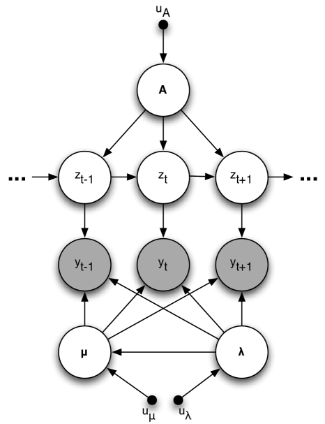
The HMM (14), illustrated in Fig. 1, models the dynamics of an observed time series ${\bf{y}}$ (here, the observed FRET ratio) as conditionally dependent on a hidden process ${\bf z}$ (here, the unknown conformational state of the molecular complex). At each time $t$, the conformational state $z_{t}$ can take on any one of $K$ possible values, conditionally dependent only on its value at the previous time via the transition probability matrix $p(z_{t}|z_{t-1})$ (i.e., ${\bf z}$ is a Markov process); the observed data depend only on the current-time hidden state via the emission probability $p(y_{t}|z_{t})$. Following the convention to the field, we model the emission probability $p(y_{t}|z_{t})$ as a Gaussian (18, 22), ignoring for the moment the complication of modeling a variable distributed on the interval $[0,1]$ with a distribution of support $(-\infty,\infty)$.

For smFRET time series with observed data $(y_{1},\ldots,y_{T})=\bm{y}$ and corresponding hidden state conformations $(z_{1},\ldots,z_{T})=\bm{z}$, the joint probability of the observed and hidden data is

$$p(\bm{y},\bm{z}|{\vec{\vartheta}},K)=p(z_{1}|{\vec{\vartheta}})\left[\prod_{t=2}^{T}p(z_{t}|z_{t-1},{\vec{\vartheta}})\right]\prod_{t=1}^{T}p(y_{t}|z_{t},{\vec{\vartheta}})$$ (7)

where ${\vec{\vartheta}}$ comprises four types of parameters: a $K$-element vector, $\vec{\pi}$ where the $k^{th}$ component, $\pi_{k}$, holds the probability of starting in the $k^{th}$ state; a $K\times K$ transition matrix, $A$, where $a_{ij}$ is the probability of transitioning from the $i^{th}$ hidden state to the $j^{th}$ hidden state (i.e. $a_{ij}=p(z_{t}=j|z_{t-1}=i)$); and two $K$-element vectors, $\vec{\mu}$ and $\vec{\lambda}$, where $\mu_{k}$ and $\lambda_{k}$ are the mean and precision of the Gaussian distribution of the $k^{th}$ state.

As in Eq. 4, the evidence follows directly from multiplying the likelihood by priors and marginalizing:

$$p(\bm{y}|K)=\sum_{\bm{z}}\int d{\vec{\vartheta}}p(\vec{\pi})p(A)p(\vec{\mu},\vec{\lambda})p(z_{1}|\vec{\pi})\left[\prod_{t=2}^{T}p(z_{t}|z_{t-1},A)\right]\prod_{t=1}^{T}p(y_{t}|z_{t},\vec{\mu},\vec{\lambda}).$$ (8)

The $p(\vec{\pi})$ and each row of A are modeled as Dirichlet distributions; each pair of $\mu_{k}$ and $\lambda_{k}$ are modeled jointly as a Gaussian-Gamma distribution. Algebraic expressions for these distributions can be found in the Supporting Material (Sec. S.2.1). Their parameter settings and the effect of their parameter settings on data inference can be found in Sec. S.2.2 and Sec. S.2.3, respectively. We found that for the experiments considered here, and the range of prior parameters tested, there is little discernible effect of the prior parameter settings on the data inference. The variational update equations approximating Eq. 8 with these priors can be found in (23).

The variational approximation to the above evidence utilizes the dynamic program termed the forward-backward algorithm (14), which requires O($K^{2}T$) computations, rendering the computation feasible. (In comparison, direct summation over all terms requires $O(K^{T})$ operations.) We emphasize that, while individual steps in the ME calculation are slightly more expensive than their ML counterparts, the scaling with the number of states and observations is identical. As discussed in section 2.3, in addition to calculating the evidence the variational solution yields a distribution approximating the probability of the parameters given the data. Idealized traces can be calculated by taking the most probable parameters from these distributions and calculating the most probable hidden state trajectory using the Viterbi algorithm (24).

3.2 Rates from states

HMMs are used to infer the number of conformational states present in the molecular complex as well as the transition rates between states. Here, we follow the convention of the field by fitting every trace individually (since the number and mean values of smFRET states often vary from traces to trace). Unavoidably then, an ambiguity is introduced comparing FRET state labels across multiple traces, since “state 2” may refer to the high variant of a low state in one trace and to the low variant of a high state in a separate trace. To overcome this ambiguity, rates are not inferred directly from $q({\vec{\vartheta}})$, but rather from the idealized traces ${\hat{\bf z}}$ where

$${\hat{\bf z}}=\operatornamewithlimits{argmax}_{{\bf z}}{q({\bf z}|{\bf{y}},\vec{\vartheta}_{\dagger},K)}$$ (9)

and $\vec{\vartheta}_{\dagger}$ are, for ME, the parameters specifying the optimal parameter distribution $q_{*}(\vec{\vartheta},{\bf z})$ or, for ML, the most likely parameters, $\vec{\vartheta}$_∗. The number of states in the data set can then be determined by combining the idealized traces and plotting a 1D FRET histogram or transition density plot (TDP). Inference facilitates the calculation of transition rates by, for example, dwell-time analysis, TDP analysis, or by dividing the sum of the dwell times by the total number of transitions (25, 18). In this work, we determine the number of states in an individual trace using ME. To overcome the ambiguity of labels when combining traces, we follow the convention of the field and use 1D FRET histograms and/or TDPs to infer the number of states in experimental data sets and calculate rates using dwell time analysis (Sec. S.1.3).

4 Numerical experiments

We created a software package to implement variational Bayes for FRET data called vbFRET. Software was written in MATLAB and is available open source, including a point and click GUI. All ME data inference was performed using vbFRET. All ML data inference was performed using HaMMy (18), although we note that any analysis based on ML should perform similarly (see Sec. S.1.1 for practicalities regarding implementing ML). Parameter settings used for both programs, methods for creating computer generated synthetic data, and methods for calculating rate constants for experimental data can be found in Sec. S.1. Following the convention of the field, in subsequent sections the dimensionless FRET ratio is quoted in dimensionless “units” of FRET.

4.1 Example: maximum likelihood vs maximum evidence

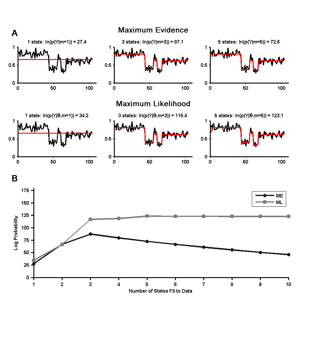
To illustrate the differences between ML and ME, consider the synthetic trace shown in Fig. 2, generated with three noisy states ($K_{0}=3$) centered at $\mu_{z}$ = (0.41, 0.61, 0.81) FRET. This trace was analyzed by both ME and ML with $K=1$ (underfit), $K=3$ (correctly fit), and $K=5$ (overfit) (Fig. 2A). In the cases when only one or three states are allowed, ME and ML perform similarly. However, when five states are allowed, ML overfits the data, whereas ME leaves two states unpopulated and correctly infers three states, illustrated clearly via the idealized trace.

Moreover, whereas the likelihood of the overfitting model is larger than that of the correct model, the evidence is largest when only three states are allowed ($p({\bf{y}}|{\vec{\vartheta}}_{*},K>K_{0})>p({\bf{y}}|{\vec{\vartheta}}_{*},K_{0})$; however, $p({\bf{y}}|K)$ peaks at $K=K_{0}=3$). The ability to use the evidence for model selection is further illustrated in Fig. 2B, in which the same data as in Fig. 2A are analyzed using both ME and ML with $1\leq K\leq 10$. The evidence is greatest when $K=3$; however, the likelihood increases monotonically as more states are allowed, ultimately leveling off after five or six states are allowed.

4.2 Statistical validation

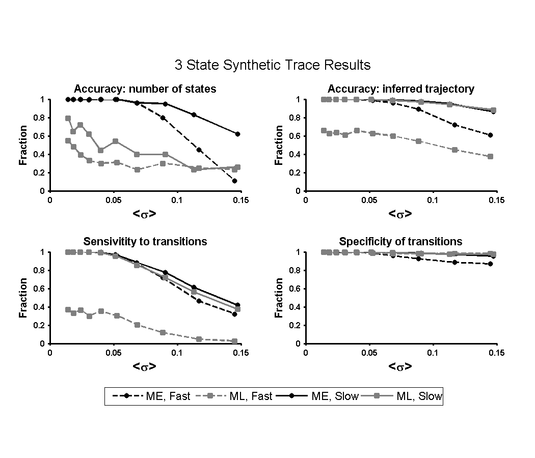
ME can be statistically validated by generating synthetic data, for which the true trajectory of the hidden state ${\bf z}_{0}$ is known, and quantifying performance relative to ML. We performed such numerical experiments, generating several thousand synthetic traces, and quantified accuracy as a function of signal-to-noise via four probabilities: (1) accuracy in number of states $p(|{{\bf{\hat{\bf z}}}}|=|{\bf z}_{0}|)$: the probability in any trace of inferring the correct number of states (where $|{\bf z}_{0}|$ is the number of states in the model generating the data and $|{{\bf{\hat{\bf z}}}}|$ is the number of populated states in the idealized trace); (2) accuracy in states $p({{\bf{\hat{\bf z}}}}={\bf z}_{0})$: the probability in any trace at any time of inferring the correct state; (3) sensitivity to true transitions: the probability in any trace at any time that the inferred trace ${{\bf{\hat{\bf z}}}}$ exhibits a transition, given that ${\bf z}_{0}$ does; and (4) specificity of inferred transitions: the probability in any trace at any time that the true trace ${\bf z}_{0}$ does not exhibit a transition, given that ${{\bf{\hat{\bf z}}}}$ does not. We note that, encouragingly, for the ME inference, $|{{\bf{\hat{\bf z}}}}|$ always equaled $K_{*}$ as defined in Eq. 2.

We identify each inferred state with the true state which is closest in terms of their means provided the difference in means is less than $0.1$ FRET. Inferred states for which no true state is within $0.1$ FRET are considered inaccurate. Note that we do not demand that one and only one inferred state be identified with the true state. This effective smoothing corrects overfitting errors in which one true state has been inaccurately described by two nearby states (consistent with the convention of the field for analyzing experimental data).

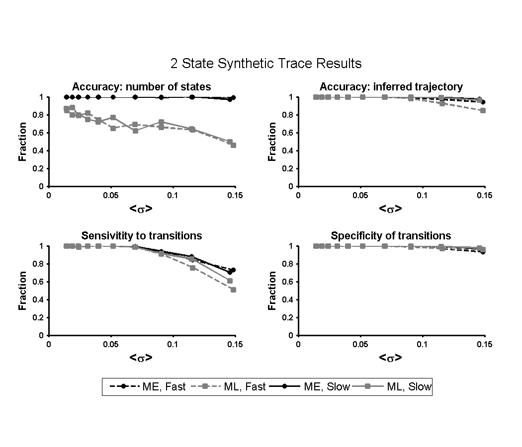
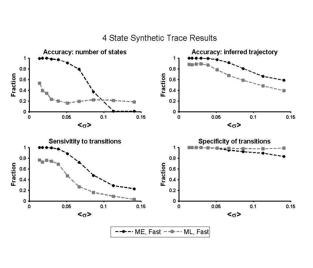
For all synthetic traces, $K_{0}$ = 3 with means centered at $\mu_{z}$ = (0.25, 0.5, 0.75) FRET. Traces were made increasingly noisy by increasing the standard deviation, $\sigma$, of each state. Ten different noise levels, ranging from $\sigma\approx 0.02$ (unrealistically noiseless) to $\sigma\approx 1.4$ (unrealistically noisy) were used. Trace length, $T$, varied from $50\leq T\leq 500$ time steps, drawn randomly from a uniform distribution. One time step corresponds to one time-binned unit of an experimental trace, which is typically 25–100 msec for most CCD camera based experiments. Fast-transitioning (mean lifetime of 4 time steps between transitions) and slow-transitioning (mean lifetime of 15 time steps between transitions) traces were created and analyzed separately. Transitions were equally likely from all hidden states to all hidden states. For each of the 10 noise levels and 2 transition speeds, 100 traces were generated (2,000 traces in total). Traces for which $K_{0}$ = 2 (Fig. S.5) and $K_{0}$ = 4 (Fig. S.6) were created and analyzed as well. The results were qualitatively similar and can be found in Sec. S.3.

As expected, both programs performed better on low noise traces than on high noise traces. ME correctly determined the number of FRET states more often than ML in all cases except for the noisiest fast-transitioning trace set (Fig. 3, top left). Of the 2,000 traces analyzed here using ME and ML, ME overfit 1 and underfit 232. ML overfit 767 and underfit 391. In short, ME essentially eliminated overfitting of the individual traces, whereas ML overfit 38% of individual traces. Over 95% (all but 9) of ME underfitting errors occurred on traces with FRET state noise $>$ 0.09, whereas ML underfitting was much more evenly distributed (at least 30 traces at every noise level were underfit by ML). The underfitting of noisy traces by ME may be a result of the intrinsic resolvability of the data, rather than a shortcoming of the inference algorithm; as the noise of two adjacent states becomes much larger than the spacing between them, the two states become indistinguishable from a single noisy state (in the limit, there is no difference between a one state and two state system if the states are infinitely noisy). The causes of the underfitting errors by ML are less easily explained, but suggest that the ML algorithm has not converged to a global optimum in likelihood (for reasons explained in Sec. S.1.2).

In analyzing the slow-transitioning traces, the methods performed roughly the same on probabilities (2–4) (always within $\sim$5% of each other). For the fast-transitioning traces, however, ME was much better at inferring the true trajectory of traces (by a factor of 1.5–1.6 for all noise levels) and showed superior sensitivity (factor of 2.7–12.5) to transitions at all noise levels. The two methods showed the same specificity to transitions until a noise level of $\sigma>$ 0.8, beyond which ML showed better specificity (factor of 1.06–1.13). Inspection of the individual traces showed that all three of these results were due to ML missing many of the transitions in the data.

These results on synthetic data suggest that when the number of states in the system is unknown, ME clearly performs better at identifying FRET states. For inference of idealized trajectories, ME is at least as accurate as ML for slow-transitioning traces and more accurate for fast-transitioning traces. The performance of ME on fast-transitioning traces is particularly encouraging since detection of a transient biophysical state is often an important objective of smFRET experiments, as discussed below.

5 Results

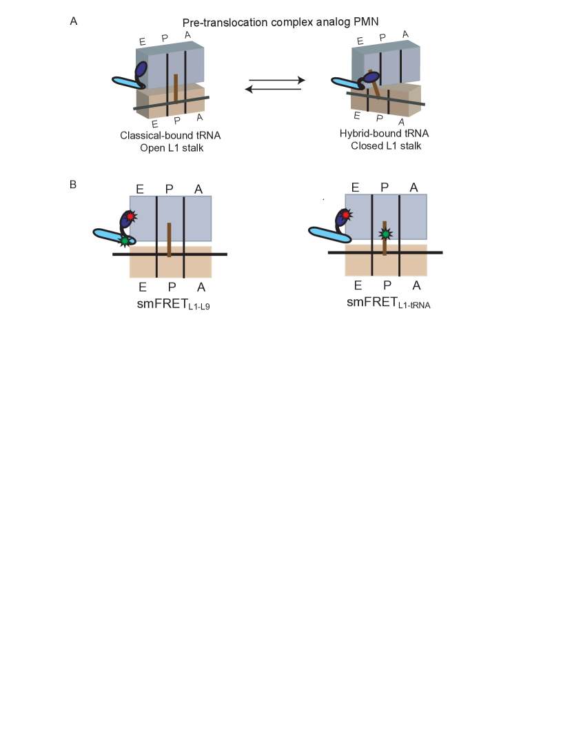
Having validated inference with vbFRET, we compared ME and ML inference on experimental smFRET data, focusing our attention on the number of states and the transition rates. The data we used for this analysis report on the conformational dynamics of the ribosome, the universally-conserved ribonucleoprotein enzyme responsible for protein synthesis, or translation, in all organisms. One of the most dynamic features of translation is the precisely directed mRNA and tRNA movements that occur during the translocation step of translation elongation. Structural, biochemical, and smFRET data overwhelmingly support the view that, during this process, ribosomal domain rearrangements are involved in directing tRNA movements (26, 27, 3, 28, 29, 6, 25, 30, 31, 32). One such ribosomal domain is the L1 stalk, which undergoes conformational changes between open and closed conformations that correlate with tRNA movements between so-called classical and hybrid ribosome-bound configurations (Fig. 4A) (6, 32, 33, 34).

Using fluorescently-labeled tRNAs and ribosomes, we have recently developed smFRET probes between tRNAs (smFRET_tRNA-tRNA) (27), ribosomal proteins L1 and L9 (smFRET_L1-L9) (6), and ribosomal protein L1 and tRNA (smFRET_L1-tRNA) (33). Collectively, these data demonstrate that, upon peptide bond formation, tRNAs within pretranslocation (PRE) ribosomal complexes undergo thermally-driven fluctuations between classical and hybrid configurations (smFRET_tRNA-tRNA) that are coupled to transitions of the L1 stalk between open and closed conformations (smFRET_L1-L9). The net result of these dynamics is the transient formation of a direct L1 stalk-tRNA contact that persists until the tRNA and the L1 stalk stochastically fluctuate back to their classical and open conformations, respectively (smFRET_L1-tRNA). This intermolecular L1 stalk-tRNA contact is stabilized by binding of elongation factor G (EF-G) to PRE and maintained during EF-G catalyzed translocation (6, 33).

Here we compare the rates of L1 stalk closing ($k_{\mathrm{close}}$) and opening ($k_{\mathrm{open}}$) obtained from ME and ML analysis of smFRET_L1-L9 PRE complex analogs (PMN) under various conditions (which have the same number of FRET states by both inference methods) and the number of states inferred for smFRET_L1-tRNA PMN complexes by ME and ML. (FRET complexes shown in Fig. 4B.) These data were chosen for their diversity of smFRET ratios. The smFRET_L1-L9 ratio fluctuates between FRET states centered at 0.34 and 0.56 (i.e. a separation of 0.22 FRET), whereas the smFRET_L1-tRNA ratio fluctuates between FRET states centered at $0.09$ and $0.59$ FRET(i.e. a separation of 0.50 FRET). In addition, smFRET_L1-L9 data were recorded under conditions that favor either fast-transitioning (PMN_fMet+EFG) or slow-transitioning (PMN_fMet and PMN_Phe) complexes (complex compositions listed in Table 1).

First, we compared the smFRET_L1-L9 data obtained from PMN_fMet, PMN_Phe, and PMN_fMet+EFG. As expected from previous studies (33), 1D histograms of idealized FRETvalues from both inference methods showed two FRETstates centered at $0.34$ and $0.56$ FRET (and one additional state due to photobleaching, for a total of three states). When individual traces were examined for overfitting, however, ML inferred four or five states in $20.1\%\pm 3.7\%$ of traces in each data set whereas ME inferred four or five states in only $0.9\%\pm 0.5$ of traces. Consequently, more post-processing was necessary to extract transition rates from idealized traces inferred by ML.

Our results (Table 1) demonstrate that there is very good overall agreement between the values of $k_{\mathrm{close}}$ and $k_{\mathrm{open}}$ calculated by ME and ML. For the relatively slow-transitioning PMN_fMet and PMN_Phe data, the values of $k_{\mathrm{close}}$ and $k_{\mathrm{open}}$ obtained from ME and ML are indistinguishable. For the relatively fast-transitioning PMN_fMet+EFG data, however, the values of $k_{\mathrm{close}}$ and $k_{\mathrm{open}}$ obtained differ slightly between ME and ML. Since the true transition rates of the experimental smFRET_L1-L9 data can never be known, it is impossible to assess the accuracy of the rate constants obtained from ME or ML in the same way we could with the analysis of synthetic data. While we cannot say which set of $k_{\mathrm{close}}$ and $k_{\mathrm{open}}$  values are most accurate for this fast-transitioning data set, our synthetic results would predict a larger difference between rate constants calculated by ME and ML for faster-transitioning data and suggest that the values of $k_{\mathrm{close}}$ and $k_{\mathrm{open}}$ calculated with ME have higher accuracy (Fig. 3).

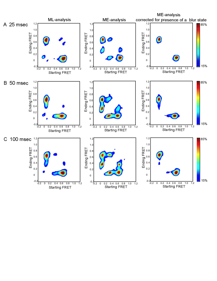
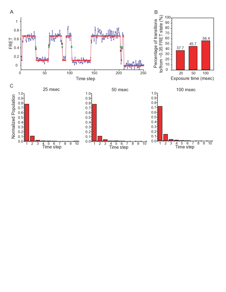
Consistent with previous reports (6), ML infers two FRET states centered at $f_{\rm low}\equiv 0.09$ and $f_{\rm high}\equiv 0.59$ FRET (plus one photobleached state) for all smFRET_L1-tRNA data sets. Conflicting with these results, however, ME infers three FRET states (plus a photobleached state) for these data sets. Two of these FRET states are centered at $f_{\rm low}$ and $f_{\rm high}$, as in the ML case, while the third “putative” state is centered at $f_{\rm mid}\equiv 0.35$ FRET, coincidentally at the mean between $f_{\rm low}$ and $f_{\rm high}$. Indeed, TDPs constructed from the idealized trajectories generated by ME or ML analysis of the PMN_fMet+EFG smFRET_L1-tRNA data set evidence the appearance of a new, highly populated state at $f_{\rm mid}$ in the ME-derived TDP that is virtually absent in the ML-derived TDP (Fig. S.7). Consistent with the TDPs, $\sim$46% of transitions in the ME-analyzed smFRET_L1-tRNA trajectories are either to or from the new $f_{\rm mid}$ state (Fig. 5B). This $f_{\rm mid}$ state is extremely short lived; $\sim$75% of the data assigned to $f_{\rm mid}$ consist of a single observation, i.e., with a duration at or below the CCD integration time (here, 50 msec) (Fig. 5C). A representative ME-analyzed smFRET_L1-tRNA trace is shown in Fig. 5A.

There are at least two possible origins for this putative new state. The first is a very short-lived (i.e. lifetime $\leq$ 50 msec), bona fide, previously unidentified intermediate conformation of the PMN complex. The second is that $f_{\rm mid}$ data are artifactual, resulting from the binning of the continuous-time FRET signal during CCD collection. Each time binned data point represents the average intensity of thousands or more photons. If a transition occurs 25 msec into a 50 msec time step, half the photons will come from the $f_{\rm low}$ state and half from the $f_{\rm high}$ state, resulting in a datum at approximately their mean. This type of CCD blurring artifact would be lost in the noise of closely spaced FRET states, but would become more noticeable as the FRET separation between states increases.

To distinguish between these two possibilities, we recorded PMN_fMet+EFG smFRET_L1-tRNA data at half and double the integration times (i.e. 25 msec and 100 msec). If the $f_{\rm mid}$ state is a true conformational intermediate then: (1) the percentage of transitions exhibiting at least one data point at or near $f_{\rm mid}$ should increase as the integration time decreases, and (2) the number of consecutive data points defining the dwell time spent at or near $f_{\rm mid}$ should increase as the integration time decreases. Conversely, if the $f_{\rm mid}$ state arises from a time averaging artifact, then: (1) the percentage of transitions containing at least one data point at or near $f_{\rm mid}$ should increase as the integration time increases, as longer integration times increase the probability that a transition will occur during the integration time, and (2) the number of consecutive data points defining the dwell time spent at or near the $f_{\rm mid}$ state should be independent of the integration time, as transitions occurring within the integration time will always be averaged to generate a single data point.

Consistent with the view that the $f_{\rm mid}$ state arises from time-averaging over the integration time, Fig. 5B demonstrates that the percentage of transitions containing at least one data point at or near $f_{\rm mid}$ increases as the integration time increases. This manifests as the increase in the density of transitions starting or ending at $f_{\rm mid}$ as the integration time decreases for the ME-derived TDPs in Fig. S.7. These data are further supported by the results presented in Fig. 5C, demonstrating that the number of consecutive data points defining the dwell time of the $f_{\rm mid}$ state is remarkably insensitive to the integration time. We conclude that the $f_{\rm mid}$ state identified by ME is composed primarily of a time-averaging artifact which we refer to as “camera blurring” and the ME-inferred $f_{\rm mid}$ state as the “blur state”. Although ML infers four or five states in 35% of the traces (compared to only 25% for ME), for some reason ML significantly suppresses, but does not completely eliminate, detection of this blur state in the individual smFRET trajectories. At present, we cannot determine whether this is a result of the ML method itself (i.e. overfitting noise in one part of the trace may cause it to miss a state in another) or due to the specific implementation of ML in the software we used (Sec. S.1.1). In retrospect, the presence of blur states should not be surprising, since they follow trivially from the time-averaging that results from averaging over the CCD integration time.

Single data point artifacts caused by stochastic photophysical fluctuations of fluorophore intensity are a well known and common problem in smFRET data (12). These artifacts can be corrected for by applying smoothing algorithms or rolling averages over the data (27, 32) or ignoring FRET states with a dwell time of one time point (6). The artifacts we encounter here are different in nature, since they result from time binning the data rather than a photophysical fluctuation in donor/acceptor signal intensity and, therefore, should be corrected for using a different approach. The algorithm we propose performs a second round of ME inference on the data, using the idealized traces from the first round of ME inference to make the following modification to the raw data: data which could have resulted from time-averaging artifacts (i.e. events lasting exactly one data point and occurring between two distinct idealized values) were moved to the idealized value closest to the value of the suspected time-averaging artifact (the assumption here is that that a single $f_{\rm mid}$ data point should be considered part of the “real” FRET state that the molecular complex spent the most time in during that transitioning time point). We performed this algorithm on the smFRET_L1-tRNA. The TDP for this “cleaned” data shows the blur state at $f_{\rm mid}$ is virtually eliminated, yielding a result that is wholly consistent with that generated by ML (Fig. S.7). In general, however, it should be cautioned that a bona fide intermediate FRET state may well exist and be buried under a strongly-populated blur state. Unless this intermediate FRET state is positively identified and somehow separated from the blur state (i.e. by obtaining data at an increased integration time), eliminating or ignoring FRET states with dwell times exactly equal to one time point may risk overlooking a bona fide intermediate FRET state. We note that the vbFRET software package which we have made available allows the user the opportunity to run this second round of ME analysis with possible blur states detected and cleaned as described above.

The observation that ML analysis does not detect a blur state that is readily identified by ME analysis is in line with our results on synthetic data in which ME consistently outperforms ML in regards to detecting the true number of states in the data, particularly in fast-transitioning data, and strongly suggests that ME will generally capture short-lived intermediate FRET states that ML will tend to overlook. While this feature of ML might be desirable in terms of suppressing blur states such as the one we have identified in the smFRET_L1-tRNA data set, it is undesirable in terms of detecting bona fide intermediate FRET states that may exist in a particular data set.

6 Conclusions

These synthetic and experimental analyses confirm that ME can be used for model selection (identification of the number of smFRET states) at the level of individual traces, improving accuracy and avoiding overfitting. Additionally, ME inference with variational Bayes provides $q_{*}$, an estimate of the true parameter and idealized trace posterior, making possible the analysis of kinetic parameters, again at the level of individual traces. As a tool for inferring idealized traces, ME produces traces which are visually similar to those of ML; in the case of synthetic data generated to emulate experimental data, ME performs with comparable or superior accuracy. The idealized trajectories inferred by ME required substantially less post-processing, however, since ME usually inferred the correct number of states to the data and, consequently, did not require states with similar idealized values within the same trace to be combined in a post-processing step. The superior trajectory inference, accuracy, and sensitivity to transitions of ME on fast transitioning synthetic traces suggests that the differences in transition rates calculated for fast transitioning experimental data is a result of superior fitting by ME as well.

In some experimental data, ME detected a very short lived blur state, which comparison of experiments at different sampling rates suggests results from a camera time averaging artifact. Once detected by ME, the presence of this intermediate state is easily confirmed by visual inspection, but yet was not identified by ML inference. Although not biologically relevant in this instance, this result suggests that ME inference is able to uncover real biological intermediates in smFRET data that would be missed by ML.

We conclude by emphasizing that this method of data inference is in no way specific to smFRET. The use of ME and variational Bayes could improve inference for other forms of biological time series where the number of molecular conformations is unknown. Some examples include motor protein trajectories with an unknown number of chemomechanical cycles (i.e. steps), DNA/enzyme binding studies with an unknown number of binding sites and molecular dynamics simulations where important residues exhibit an unknown number of rotamers.

All code used in this analysis, as well as a point and click GUI interface, is available open source via http://vbFRET.sourceforge.net.

7 Acknowledgments

It is a pleasure to acknowledge helpful conversations with Taekjip Ha and Vijay Pande, Harold Kim and Eric Greene for comments on the manuscript, mathematical collaboration with Alexandro D. Ramirez, and Subhasree Das for managing the Gonzalez laboratory. This work was supported by a grant to CHW from the NIH (5PN2EY016586-03) and grants to RLG from the Burroughs Wellcome Fund (CABS 1004856), the NSF (MCB 0644262), and the NIH-NIGMS (1RO1GM084288-01).

Table 1: Comparison of smFRET_L1-L9 transition rates inferred by ME and ML

Data set∗	Method	$k_{\mathrm{close}}$	$k_{\mathrm{open}}$
PMNPhe†	ME	$0.66\pm 0.05$	$1.0\pm 0.2$
	ML	$0.65\pm 0.06$	$1.0\pm 0.3$
PMNfMet‡	ME	$0.53\pm 0.08$	$1.7\pm 0.3$
	ML	$0.52\pm 0.06$	$1.8\pm 0.3$
PMNfMet+EFG	ME	$3.1\pm 0.6$	$1.3\pm 0.2$
($1\mu M$)§	ML	$2.1\pm 0.4$	$1.0\pm 0.2$
PMNfMet+EFG	ME	$2.6\pm 0.6$	$1.5\pm 0.1$
($0.5\mu M$)§	ML	$2.0\pm 0.3$	$1.0\pm 0.1$

^∗ Rates reported here are the average and standard deviation from three or four independent data sets. Rates were not corrected for photobleaching of the fluorophores.

^† PMN_Phe was prepared by adding the antibiotic puromycin to a post-translocation complex carrying deacylated-tRNA^fMet at the E site and fMet-Phe-tRNA^Phe at the P site, and thus contains a deacylated-tRNA^Phe at the P site.

^‡ PMN_fMet was prepared by adding the antibiotic puromycin to an initiation complex carrying fMet-tRNA^fMet a the P site, and thus contains a deacylated-tRNA^fMet at the P site.

^§ 1.0 $\mu M$ and 0.5 $\mu M$ EF-G in the presence of 1 mM GDPNP (a non-hydrolyzable GTP analog) were added to PMN_fMet, respectively.

Figure 1: Graphical model representation of the HMM, corresponding to the factorization of the probability distribution in Eq. 7. Each vertical slice represents a time slice $t=1,\ldots,T$, for which there is an observed FRET ratio $y_{t}$, given a hidden conformational state $z_{t}\in 1,\ldots,K$. Transitions between conformational states are represented by the dependencies between $z_{t}$ and $z_{t-1}$. Parameters are also shown as random variables, with arrows indicating the dependence of the observed and hidden variables. Parameters for the probability distributions over parameters (Sec. S.2.2) are shown as solid black circles.

Figure 2: A single (synthetic) FRET trace analyzed by ME and ML. The trace contains 3 hidden states. A) (Top) idealize traces inferred by ME when $K=1,K=3$, and $K=5$, as well as the corresponding log(evidence) for the inference. The data are under resolved when $K=1$, but for both $K=3$ and $K=5$ the correct number of states are populated. (Bottom) idealized traces inferred by ML when $K=1,K=3$, and $K=5$, as well as the corresponding log(likelihood). Inference when $K=1$ and $K=3$ are the same as for ME but the data are overfit when $K=5$. B) The log evidence from ME (black) and log likelihood from ML (gray) for $1\leq K\leq 10$. The evidence is correctly maximized for $K=3$, but the likelihood increases monotonically.

Figure 3: Comparison of ME and ML as a function of increasing hidden state noise. Fast transitioning (hidden state mean lifetime of 4 time steps) and slow transitioning (hidden state mean lifetime of 15 time steps) traces were created and analyzed separately. Each data point represents the average value taken over 100 traces. (Top left) $p(|{{\bf{\hat{\bf z}}}}|=|{\bf z}_{0}|)$: the probability in any trace of inferring the correct number of states. (Top right) $p({{\bf{\hat{\bf z}}}}={\bf z}_{0})$: the probability in any trace at any time of inferring the correct state. (Bottom left) sensitivity to true transitions: the fraction of time the correct FRET state was inferred during FRET trajectories. (Bottom right) specificity of inferred transitions: the probability in any trace at any time that the true trace ${\bf z}_{0}$ does not exhibit a transition, given that ${{\bf{\hat{\bf z}}}}$ does not. Error bars on all plots were omitted for clarity and because the data plotted represent mean success rates for Bernoulli processes (and, therefore, determine the variances of the data as well).

Figure 4: Conformational rearrangements within a pre-translocation (PMN) complex and smFRET labeling schemes. (A) Cartoon representation of a PMN complex analog. The small and large ribosomal subunits are shown in tan and lavender, respectively, with the L1 stalk depicted in dark blue, and ribosomal protein L9 in cyan. The aminoacyl-, peptidyl- and deacylated-tRNA binding sites are labeled as A, P and E, respectively, and the P-site tRNA is depicted as a brown line. PMN complex analogs are generated by adding the antibiotic puromycin to a post-translocation complex carrying a deacylated-tRNA at the E site and a peptidyl-tRNA at the P site. The resulting PMN complex analog exists in a thermally-driven dynamic equilibrium between two major conformational states in which the P-site tRNA fluctuations between classical and hybrid configurations correlate with the L1 stalk fluctuations between open and closed conformations. (B) Two labeling schemes have been developed in order to investigate PMN complex dynamics using smFRET. PMN complexes are cartooned as in (A) with Cy3 and Cy5 depicted as green and red stars, respectively. smFRET_L1-L9 (left), which involves a Cy5 label on ribosomal protein L1 within the L1 stalk and a Cy3 label on ribosomal protein L9 at the base of the L1 stalk, reports on the intrinsic conformational dynamics of the L1 stalk. smFRET_L1-tRNA (right), which involves a Cy5 label on ribosomal protein within the L1 stalk as in smFRET_L1-L9 and a Cy3 label on the P-site tRNA, reports on the formation and disruption of a direct interaction between the closed L1 stalk and the hybrid bound P-site tRNA.

Figure 5: Analysis of the smFRET_L1-tRNA $f_{\rm mid}$ state. A) A representative smFRET_L1-tRNA trace idealized by ME, taken from the 50 msec exposure time data set. Both the observed data (blue) and idealized path (red) are shown. Individual data points, real and idealized, are shown as Xs. To emphasize the data at or near $f_{\rm mid}$, the Xs are enlarged and the observed and idealized data are show in black and green, respectively. (B) Bar graph of the percentages of transitions to or from the $f_{\rm mid}$ state under 25 msec, 50 msec and 100 msec CCD integration time. (C) Normalized population histograms of dwell time spent at the $f_{\rm mid}$ state under 25 msec, 50 msec, and 100 msec CCD integration time.

Appendix A $\chi^{2}$ and maximum likelihood

Minimization of squared loss is most commonly derived in the natural sciences by asserting that ‘error’, the difference between parameterized model prediction and experimental data, is additive, normally distributed, and independent for each example (here indexed by $i$):

$$y_{i}=f_{\vartheta}(x_{i})+\xi_{i};~{}~{}\xi_{i}\sim\mathcal{N}(\xi|0,\sigma).$$ (10)

This notation emphasizes that the model $f$ depends on parameters $\vartheta$, and the $\sim$ indicates the distribution from which the error $\xi_{i}$ on the $i^{\rm th}$ observation is drawn (i.e., the Gaussian or normal distribution and variance $\sigma$). Assuming independent and identically distributed observations, the probability of all the $N$ data ${\bf y}=\{y_{i}\}_{i=1}^{i=N}$ is then the likelihood

$$L=p({\bf y}|\vartheta)=\Pi_{i=1}^{i=N}\mathcal{N}(y_{i}-f_{\vartheta}(x_{i})|0,\sigma)=\frac{{\rm e}^{-\chi^{2}}}{(\sqrt{2\pi\sigma})^{N}}$$ (11)

with the usual $\chi^{2}=\sum_{i=1}^{i=N}(y_{i}-f_{\vartheta}(x_{i}))^{2}/\sigma^{2}$ arising as a linear term in the logarithm of the likelihood $\ell$:

$$\ell\equiv\ln L=-\chi^{2}+{\frac{N}{2}}\ln 2\pi\sigma.$$ (12)

Minimization of $\chi^{2}$, is thus derived from the more general principle of ML: the parameters $\vartheta_{*}$ chosen are those which are the most likely.

Appendix B “BIC”: an intuition-building heuristic

Often, explicit calculation of $p({\bf{y}}|K)$ is computationally difficult, and one resorts to approximation. For example, if the likelihood $p({\bf{y}}|{\vec{\vartheta}},K)$ is sharply and uniquely peaked as a function of ${\vec{\vartheta}}^{K}$, meaning that there is one unique maximum, Schwartz (35) suggested a pair of approximations: (i) Taylor expansion of $\ell({\vec{\vartheta}})$ (from Eq. 12) and Laplace approximation of the integral; and (ii) replacing the second derivative of $\ell({\vec{\vartheta}})$ by its asymptotic behavior in the limit $\{K,N\}\rightarrow\infty$. The first approximation reads

$$p({\bf{y}}|K)=\int d^{K}{\vec{\vartheta}}{{\rm e}^{\ell({\vec{\vartheta}})}}p({\vec{\vartheta}}|K)\approx{\rm e}^{\ell_{*}}p({\vec{\vartheta}}_{*}|K)\sqrt{\left|\frac{2\pi}{H}\right|}$$ (13)

where $\ell_{*}=\ell(\vartheta_{*})$ is the ML over all parameters $\vartheta$, and the $K\times K$ matrix $H$, also termed the Hessian, is the matrix of derivatives (evaluated at ${\vec{\vartheta}}_{*}$)

$$H_{\alpha\beta}\equiv\frac{\partial^{2}\ell(\bf\vartheta)}{\partial\vartheta_{\alpha}\partial\vartheta_{\beta}}.$$ (14)

In the case of independent data the derivative of $\ell$ is a sum of $N$ independent terms, and the determinant of the Hessian scales as $N^{K}$ in the limit of infinite data $N$ and infinitely many $K$ equally-important parameters $\vartheta_{\alpha}$. Under this pair of asymptotic approximations, then,

$$p({\bf{y}}|K)\approx{\rm e}^{\ell_{*}}p({\vec{\vartheta}}_{*}|K)\sqrt{\left|\frac{2\pi}{H}\right|}\approx C(K,N){\rm e}^{(\ell_{*}-K/2\ln N)}.$$ (15)

The exponent is sometimes referred to as the Bayesian Information Criterion or BIC; for clarity it is worth noting, though, that it does not depend on the prior (the most common meaning of the adjective ‘Bayesian’ in statistics) and that it is derived without any appeal to or use of information theory. The usage of such an algebraic expression alone, ignoring the possible dependence of terms lumped into $C(K,N)$ (i.e., treating $C(K,N)$ as a constant) is a simple, intuitive, and appealing approach to model selection. The increase in $\ell_{*}$ as $K$ increases is penalized by the term $-K/2\ln N$, selecting the optimal model indexed by $K_{*}$, the maximizer of the BIC.

In the case of FRET data the likelihood is complicated by the presence of a hidden state $z_{i}$ (the discrete conformational state of the molecule which gives rise to the observed FRET ratio), meaning that the evidence $p({\bf{y}}|K)$ has the richer formulation (suppressing the cluttering superscripts $K$ on the hidden and manifest variables $z$ and $\vartheta$, respectively)

$$p({\bf{y}}|K)=\sum_{\bf z}\int d^{K}{\vec{\vartheta}}p({\bf{y}},{\bf z}|{\vec{\vartheta}},K)p({\bf z}|{{\vec{\vartheta}}},K)p({\vec{\vartheta}}|K).$$ (16)

This rich structure renders completely inappropriate the assumptions of the BIC derivation above: among other problems, the hidden variables will be modeled by a Markovian dynamic, coupling each of the example data (and thus violating the assumption of $N$ independent data); and the permutation symmetry of the labels on these violates the assumption that the likelihood is sharply and singly peaked – rather there are $K!$ such peaks from the possible re-labelings of the states.

Appendix C Proof of variational relation

We provide a proof of the variational relation in Eq. 6. We start with the desired quantity, the evidence $p({\bf{y}}|K)$, and multiply by one,

$$\ln p({\bf{y}}|K) = \left[\sum_{\bm{z}}\int d\vartheta q({\bf z},{\vec{\vartheta}})\right]\ln p({\bf{y}}|K),$$ (17)

valid for any normalized probability distribution $q({\bf z},{\vec{\vartheta}})$. We then use the definition of conditional probability to write

$$p({\bf{y}},{\vec{\vartheta}},{\bf z}|K)=p({\bf z},{\vec{\vartheta}}|{\bf{y}},K)p({\bf{y}}|K).$$ (18)

We use this to rewrite the argument of the logarithm and multiply by one yet again:

$$\ln p({\bf{y}}|K) = \sum_{\bm{z}}\int d\vartheta q({\bf z},{\vec{\vartheta}})\ln\left[{p({\bf{y}},{\vec{\vartheta}},{\bf z}|K)\over p({\bf z},{\vec{\vartheta}}|{\bf{y}},K)}\right]$$ (19)

$$= \sum_{\bm{z}}\int d\vartheta q({\bf z},{\vec{\vartheta}})\ln\left[{p({\bf{y}},{\vec{\vartheta}},{\bf z}|K)q({\bf z},{\vec{\vartheta}})\over q({\bf z},{\vec{\vartheta}})p({\bf z},{\vec{\vartheta}}|{\bf{y}},K)}\right]$$ (20)

$$= \sum_{\bm{z}}\int d\vartheta q({\bf z},{\vec{\vartheta}})\ln\left[{p({\bf{y}},{\vec{\vartheta}},{\bf z}|K)\over q({\bf z},{\vec{\vartheta}})}\right]+\sum_{\bm{z}}\int d\vartheta q({\bf z},{\vec{\vartheta}})\ln\left[{q({\bf z},{\vec{\vartheta}})\over p({\bf z},{\vec{\vartheta}}|{\bf{y}},K)}\right],$$ (21)

where in the last line we have separated logarithm to decompose the integral into two parts. We recognize the rightmost term as the Kullback-Leibler divergence between $q({\bf z},{\vec{\vartheta}})$ and $p({\bf z},{\vec{\vartheta}}|{\bf{y}},K)$,

$$D_{KL}(q({\bf z},{\vec{\vartheta}})||p({\bf z},{\vec{\vartheta}}|{\bf{y}},K)) = \sum_{\bm{z}}\int d\vartheta q({\bf z},{\vec{\vartheta}})\ln\left[{q({\bf z},{\vec{\vartheta}})\over p({\bf z},{\vec{\vartheta}}|{\bf{y}},K)}\right]$$ (22)

and define the remaining term as the negative of the free energy,

$$F[q({\bf z},{\vec{\vartheta}})]=-\sum_{\bm{z}}\int d\vartheta q({\bf z},{\vec{\vartheta}})\ln\left[{p({\bf{y}},{\vec{\vartheta}},{\bf z}|K)\over q({\bf z},{\vec{\vartheta}})}\right],$$ (23)

which results in the variational relation presented in Eq. 6,

$$\ln p({\bf{y}}|K) = -F[q({\bf z},{\vec{\vartheta}})]+D_{KL}(q({\bf z},{\vec{\vartheta}})||p({\bf z},{\vec{\vartheta}}|{\bf{y}},K)).$$ (24)

This completes the proof of the variational relation and offers several insights.

The first is that the free energy is strictly bounded by the log-evidence, as the Kullback-Leibler (KL) divergence is a non-negative quantity, proven through an application of Jensen’s inequality (36) (an extension of the definition of convexity). Thus we have reduced the problem of approximating the evidence to that of finding the distribution $q({\bf z},{\vec{\vartheta}})$ which is “closest” to the true (and intractable) posterior $p({\bf z},{\vec{\vartheta}}|{\bf{y}},K)$ in the KL sense. As per Eq. 24, we see that this is equivalent to minimizing the free energy $F[q({\bf z},{\vec{\vartheta}})]$ as a functional of $q({\bf z},{\vec{\vartheta}})$. This observation motivates the variational Bayes Expectation Maximization algorithm, in which a specific factorization for $q({\bf z},{\vec{\vartheta}})$ is chosen as to make calculation of $F[q({\bf z},{\vec{\vartheta}})]$ tractable, and iterative coordinate ascent is performed to find a local minimum.

In addition, we provide motivation for the term “free energy”, rewriting Eq. 23 by decomposing the logarithm:

$$F[q({\bf z},{\vec{\vartheta}})] = -\sum_{\bm{z}}\int d\vartheta q({\bf z},{\vec{\vartheta}})\ln\left[{p({\bf{y}},{\vec{\vartheta}},{\bf z}|K)\over q({\bf z},{\vec{\vartheta}})}\right]$$ (25)

$$= -\sum_{\bm{z}}\int d\vartheta q({\bf z},{\vec{\vartheta}})\ln p({\bf{y}},{\vec{\vartheta}},{\bf z}|K)+\sum_{\bm{z}}\int d\vartheta q({\bf z},{\vec{\vartheta}})\ln q({\bf z},{\vec{\vartheta}}).$$ (26)

Recognizing the negative log-probability in the first term as an energy (as in the Boltzmann distribution) and the second term as the information entropy (37, 38) of $q({\bf z},{\vec{\vartheta}})$, i.e.

$$E \equiv -\ln p({\bf{y}},{\vec{\vartheta}},{\bf z}|K)$$ (27)

$$S \equiv -\sum_{\bm{z}}\int d\vartheta q({\bf z},{\vec{\vartheta}})\ln q({\bf z},{\vec{\vartheta}}).$$ (28)

Thus we can rewrite 23 as

$$F=\langle E\rangle-TS,$$ (29)

(with unit “temperature” T) where the angled brackets denote expectation under the variational distribution $q({\bf z},{\vec{\vartheta}})$. This familiar form from statistical physics offers the following interpretation: in approximating the evidence (and posterior), we seek to minimize the free energy by finding a distribution $q({\bf z},{\vec{\vartheta}})$ that balances minimizing the energy and maximizing entropy.

We encourage the reader to enjoy the texts (19) and (20) for more pedagogical discussions of variational methods.

Appendix S Supporting material

S.1 Methods

S.1.1 ML inference settings

Following the HaMMy user manual, ML analyses use $K_{max}+2$ states, where $K_{max}$ is either $K_{0}$ (the true number of states) in the case of synthetic data or simply 3 in the case of experimental data, as 1D FRET histograms suggest two biophysical states and one photophysical state: the photobleached state. No additional complexity control was applied to the resulting parameters inferred from individual traces. The default guess for the initial distribution of the means $\mu_{z}$ was used, i.e., uniform spacing between $0$ and $1$ FRET.

Also consistent with default settings, we use the parameters inferred using only one set of initial parameter-guesses. Note that this differs from the usual implementation of expectation-maximization as a technique for performing ML (cf., (20)). Expectation-maximization (the maximization technique used in both HaMMy and vbFRET) provably converges to a local optimum, and therefore the maximization typically is performed using many random restarts for parameter values. One possible reason to avoid this procedure is the inescapable pathology of ML for real-valued emissions (e.g., in FRET data) and for which the width of each state is an inferred parameter: the optimization is ill-posed since the case in which one observation is assigned to a state of 0 uncertainty is infinitely likely (cf., (20) Ch. 9: “These singularities provide another example of the severe overfitting that can occur in a maximum likelihood approach. We shall see that this difficulty does not occur if we adopt a Bayesian approach.”).

S.1.2 ME inference settings

In analyzing synthetic and experimental data with ME, we attempt each choice of $K=1,2,\ldots,K_{\rm max}+2$ with $K_{\rm max}$ as above. For synthetic data, 25 random initial guesses were used for each of the traces; for experimental data, 100 initializations were used (though, in our experience, little or no change in the optimization was found after 25 initializations). As with all local optimization techniques, including expectation maximization in ML or in ME, we use the parameters which give the optimum over all restarts (here, the set of parameters specifying the approximating distribution $q$ which gives the maximum evidence $p({\bf{y}}|K)$).

S.1.3 Rate constant calculations

Rates for the smFRET_L1-L9 experimental data, both for ME and ML analyses, were extracted as previously described (6, 34). First, the set of all idealized traces over all times is histogrammed into 50 bins, evenly spaced between $-0.2$ and $1.2$ FRET. The counts in the resulting histogram are given to Origin 7.0, which learns a Gaussian mixture model via expectation-maximization, using user-supplied initial guesses for the three means (we used $\mu=(0,0.35,0.55)$ FRET). Origin returns true means and variances for each of the 3 states. From these variances the width at half-max for each mixture is determined, defining three acceptable ranges of fret values. (For this experiment, these ranges had widths of approximately $.05$ FRET. We next re-scan the idealized traces and, for each transition from one acceptable range to another, record the dwell time (the total time spent within the range; any number of inferred transition within one accepted range are ignored, effectively smoothing of overfit idealized traces). The cumulative distribution of dwell times from a given state is now given to Origin 7.0 to infer the most likely parameters, asserting exponential decay. The inverse of the inferred time constant is the rate constant reported for that state.

S.1.4 Generating synthetic data

Synthetic data were generated in MATLAB. Rather than testing the inference on data generated precisely by the emissions model (one in which the scalar FRET signal is taken to be normally-distributed in each state), we challenge the inference by using a slightly more realistic distribution: one that is normally-distributed in each of the two florophore colors. That is, each synthetic trace was created from a hidden Markov model with 2D Gaussian output (representing the two florophore colors). The 2D data $\bm{x}_{1},\bm{x}_{2}$ were then FRET transformed using $\bm{f}=\bm{x}_{2}/(\bm{x}_{1}+\bm{x}_{2})$; points such that $f\notin(0,1)$ were discarded.

The 2D Gaussians are chosen so that, in any state $z$, the sum of the means is 1000 ($\mu_{z}^{1}+\mu_{z}^{2}=1000\ \forall z$), roughly corresponding to our experimental data. Variances were drawn from a uniform distribution centered at each dimension’s mean over a range given by 10% of the mean. The two components were allowed a nonzero covariance, also drawn from a uniform distribution centered at 0, with a range given by $1/2$ the smaller of the two means. We emphasize that these choices are intended both to be consistent with the smFRET_L1-L9 and smFRET_L1-tRNA data and not to match the algebraic expressions in the priors used below, which would be a less challenging inference task (model specification identically matching the generative process).

Increasingly noisy traces were generated by multiplying the covariance matrix of each hidden state by a constant. Ten constants, chosen log-linearly between 1 and 100, were used. The mean standard deviation of the FRET state noise in the resulting 1D traces varied from, approximately, $0.02<\sigma<1.4$.

S.2 Priors

S.2.1 Mathematical expressions for priors

To calculate the model evidence, we treat the components of ${\vec{\vartheta}}$ as random variables. The vector $\vec{\pi}$ and each row of A are modeled as Dirichlet distributions:

$$p(\vec{\pi}) = \frac{\Gamma(\sum_{k=1}^{K}u_{\pi}^{k})}{\prod_{k=1}^{K}\Gamma(u_{\pi}^{k})}\prod_{k=1}^{K}\pi_{k}^{u_{\pi}^{k}-1}$$ (30)

$$p(a_{j1},...,a_{jK}) = \frac{\Gamma(\sum_{k=1}^{K}u_{a}^{jk})}{\prod_{k=1}^{K}\Gamma(u_{a}^{jk})}\prod_{k=1}^{K}a_{jk}^{u_{a}^{jk}-1}$$ (31)

The probabilities for each pair of $\mu_{k}$ and $\lambda_{k}$ are modeled jointly as a Gaussian-Gamma distribution:

$$p(\mu_{k},\lambda_{k})=\sqrt{\frac{u_{\beta}^{k}\lambda_{k}}{2\pi}}e^{-\frac{1}{2}u_{\beta}^{k}\lambda_{k}(\mu_{k}-u_{\mu}^{k})^{2}}\frac{1}{\Gamma(u_{v}^{k}/2)}(2u_{W}^{k})^{-u_{v}^{k}/2}\lambda_{k}^{(u_{v}^{k}/2)-1}e^{-\frac{\lambda_{k}}{2u_{W}^{k}}}.$$ (32)

The terms ${\vec{u}_{\pi}}$, $\vec{u}_{a}$, $\vec{u}_{\beta}$, $\vec{u}_{\mu}$, $\vec{u}_{v}$, and $\vec{u}_{W}$ are called the hyperparameters for the probability distributions over ${\vec{\vartheta}}$.

S.2.2 Hyperparameter settings

Hyperparameters for vbFRET were set so as to give distributions consistent with experimental data and to influence the inference as weakly as possible: $u_{\pi}^{k}=1$, $u_{a}^{jk}=1$, $u_{\beta}^{k}=0.25$, $u_{m}^{k}=0.5$, $u_{v}^{k}=5$ and $u_{W}^{k}=50$, for all values of k. Qualitatively, these hyperparameters priors correspond to probability distributions over the hidden states such that it is most probable that the hidden states are equally likely to be occupied and equally likely to be transitioned to. Quantitatively, they yield $\langle\mu_{k}\rangle=0.5$ and typical $\sigma\approx 0.08$, consistent with experimental observation. ($1/\sqrt{{\rm mode}(\lambda_{k})}=1/\sqrt{150}\approx 0.08~{}\forall k$).

S.2.3 Sensitivity to hyperparameter settings

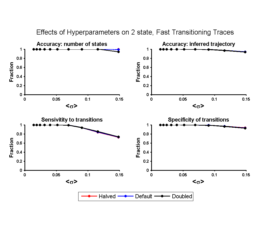
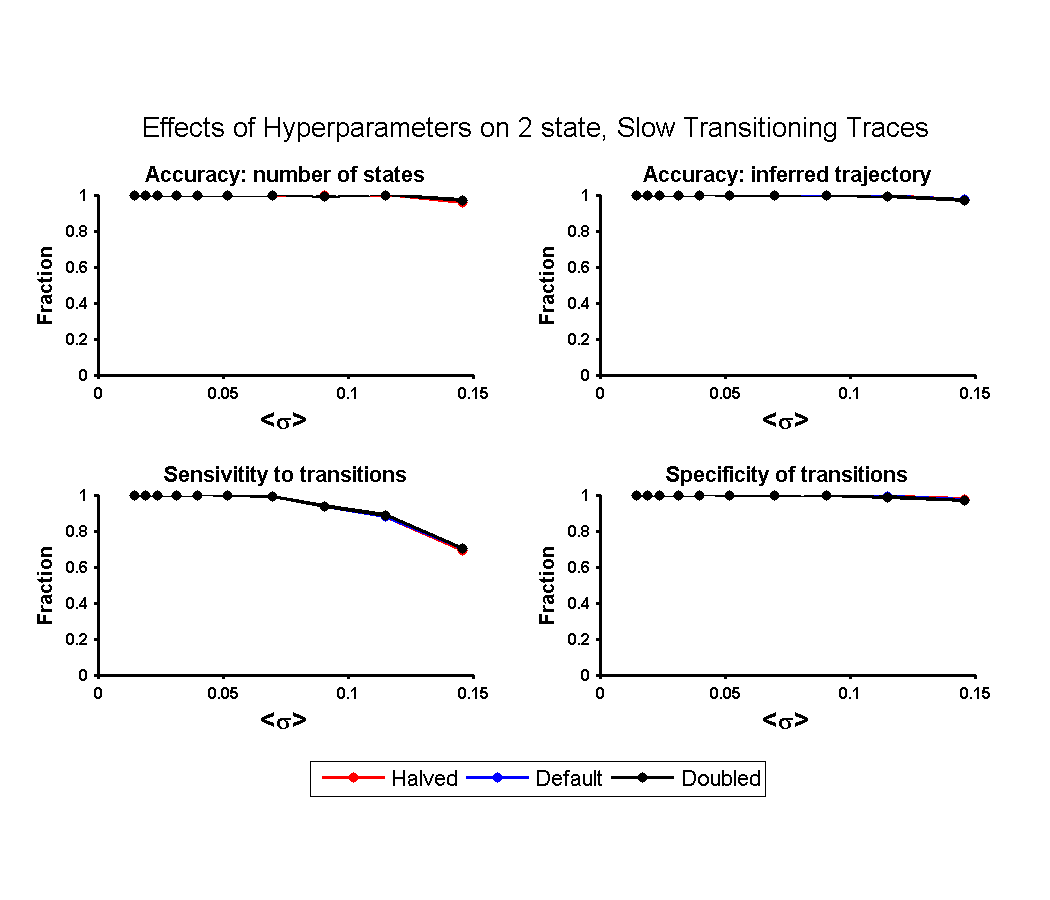
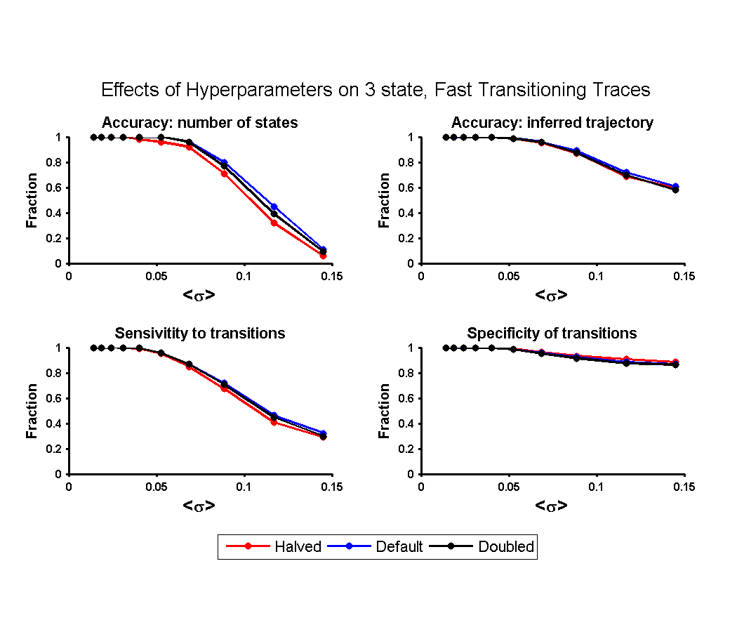
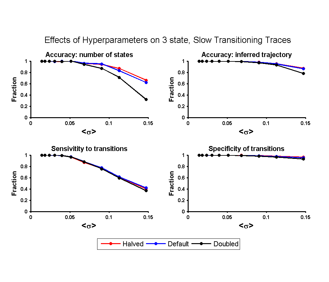
One standard approach (39, 40) to sensitivity analysis is to halve and double hyperparameters and recompute the evidence for different models. The sensitivity of ME inference on hyperparameter settings was investigated on both experimental and synthetic data. First, the two and three state traces from Fig. 3 and Fig. S.5 were reanalyzed with all the hyperparameters set to one half their default values and twice their default values (Figs. S.1, S.2, S.3, S.4). One hyperparameter, the prior on the mean of each Gaussian, was not changed during this analysis, since its value is set to 0.5 based on a symmetry argument.

The results show a relative insensitivity to the hyperparameter values over the settings considered. The largest difference in inference accuracy between the different settings was for the noisy, slow-transitioning traces shown in Fig. S.4, when the hyperparameters were doubled. Interestingly, these traces are harder to resolve than the two state traces but not as difficult to resolve as the noisy, fast-transitioning three state traces. A possible explanation for this behavior is that the two state trace results are insensitive to hyperparameter settings because the data are easy enough to resolve and the noisy, fast-transitioning three state traces are insensitive to hyper parameter settings because they are too hard to resolve. The noisy, slow-transition states are on the border of being resolvable, so using a prior that more closely matches the true parameters of the model yields more accurate results. Additionally, the three state, slow-transition data has the highest probability of having a sparsely populated state (i.e. one that is only present for a few time steps in a trace). When $\sigma$ is large, these sparsely populated states become harder to identify as distinct states, which may explain why $p(|\hat{{\bf z}}|=|{\bf z}_{0}|)$ decreases more than $p(\hat{{\bf z}}={\bf z}_{0})$, sensitivity or specificity .

Figure S.1: Effects of hyperparameter settings on fast-transitioning, two state traces.

Figure S.2: Effects of hyperparameter settings on slow-transitioning, two state traces.

Figure S.3: Effects of hyperparameter settings on fast-transitioning, three state traces.

Figure S.4: Effects of hyperparameter settings on slow-transitioning, three state traces.

To investigate further the effects of the hyperparameter settings on ME inference, the experimental data from Table 1 were reanalyzed using a more strongly diagonal transition matrix prior (Table S.1). In this second prior, the diagonal terms of the transition matrix were set to 1 and the off-diagonal terms were set to 0.05, loosely corresponding to a prior belief that the ribosome was 10x more likely to remain in its current state than transition to a new one. For all of the data, the transition rates calculated with both hyperparameter settings are within error of each other for all transition rates.

Table S.1: Effect of hyperparameters on transition rate inference

Data set∗	Settings	$k_{\mathrm{close}}$	$k_{\mathrm{open}}$
PMNPhe†	Default	$0.66\pm 0.05$	$1.0\pm 0.2$
	Diagonal	$0.66\pm 0.04$	$1.0\pm 0.2$
PMNfMet‡	Default	$0.53\pm 0.08$	$1.7\pm 0.3$
	Diagonal	$0.52\pm 0.09$	$1.7\pm 0.1$
PMNfMet+EFG	Default	$3.1\pm 0.6$	$1.3\pm 0.2$
($1\ \mu M$)§	Diagonal	$2.8\pm 0.5$	$1.3\pm 0.1$
PMNfMet+EFG	Default	$2.6\pm 0.6$	$1.5\pm 0.1$
($0.5\ \mu M$)§	Diagonal	$2.6\pm 0.5$	$1.4\pm 0.1$

^∗ Rates reported here are the average and standard deviation from three or four independent data sets. Rates were not corrected for photobleaching of the fluorophores.

^† PMN_Phe was prepared by adding the antibiotic puromycin to a post-translocation complex carrying deacylated-tRNA^fMet at the E site and fMet-Phe-tRNA^Phe at the P site, and thus contains a deacylated-tRNA^Phe at the P site.

^‡ PMN_fMet was prepared by adding the antibiotic puromycin to an initiation complex carrying fMet-tRNA^fMet a the P site, and thus contains a deacylated-tRNA^fMet at the P site.

^§ 1.0 $\mu M$ and 0.5 $\mu M$ EF-G in the presence of 1 mM GDPNP (a non-hydrolyzable GTP analog) were added to PMN_fMet, respectively.

S.3 Synthetic validation – 2 and 4 state traces

Synthetic data for 2 FRET state traces (fast- and slow-transitioning, smFRET state means at 0.3 and 0.7 FRET) and 4 FRET state traces (fast-transitioning only, smFRET state means at 0.21, 0.41, 0.61 and 0.81 FRET) were generated and analyzed exactly as the traces in Fig. 2. The results are qualitatively similar to those in Fig. 2. Inference accuracy begins to decrease at a lower noise level as more FRET states are added to the traces. This should not be surprising, though, since the states are more closely spaced as the number of states increases, and therefore should be harder to resolve.

Figure S.5: Synthetic results for two state traces.

Figure S.6: Synthetic results for four state traces.

S.4 Blur state TDPs

Figure S.7: Transition density plots (TDP) of smFRET_L1-tRNA PMN_fMet+EF-G derived from ME and ML analysis with different CCD integration times. TDPs are contour plots showing the kernel density estimation of the transitions in idealized traces (with starting and ending FRET values of the transitions as the X and Y axes, respectively). Note that transitions to short-lived or nearby states count with equal weight as those to long-lived states in a TDP. This should not be confused with a time-density plot, which illustrates the probability of observing a pair of experimental values at two different times $p(y(t),y(t+\delta t))$, which can be made from the FRET data themselves without appealing to statistical inference. The plots show ML (left), ME (middle) and ME analysis corrected for the presence of a blur state (right) Contours are plotted from tan (lowest population) to red (highest population). Different CCD integration times were used for recoding these data sets: (A) 25 msec, (B) 50 msec, and (C) 100 msec. For interpretation of the significance of these TDPs, cf. Sec. 5.

References

- Koster et al. (2006) Koster, D., C. Wiggins, and N. Dekker, 2006. Multiple events on single molecules: Unbiased estimation in single-molecule biophysics. Proceedings of the National Academy of Sciences of the United States of America 103:1750–1755.
- Moffitt et al. (2009) Moffitt, J. R., Y. R. Chemla, K. Aathavan, S. Grimes, P. J. Jardine, D. L. Anderson, and C. Bustamante, 2009. Intersubunit coordination in a homomeric ring ATPase. Nature 457:446–U2.
- Munro et al. (2007) Munro, J. B., R. B. Altman, N. O’Connor, and S. C. Blanchard, 2007. Identification of two distinct hybrid state intermediates on the ribosome. Molecular Cell 25:505–517.
- Zhuang et al. (2000) Zhuang, X. W., L. E. Bartley, H. P. Babcock, R. Russell, T. J. Ha, D. Herschlag, and S. Chu, 2000. A single-molecule study of RNA catalysis and folding. Science 288:2048–+.
- Zhuang et al. (2002) Zhuang, X. W., H. Kim, M. J. B. Pereira, H. P. Babcock, N. G. Walter, and S. Chu, 2002. Correlating structural dynamics and function in single ribozyme molecules. Science 296:1473–1476.
- Fei et al. (2008) Fei, J., P. Kosuri, D. D. MacDougall, and R. L. Gonzalez, 2008. Coupling of ribosomal L1 stalk and tRNA dynamics during translation elongation. Molecular Cell 30:348–359.
- Yildiz et al. (2004) Yildiz, A., M. Tomishige, R. D. Vale, and P. R. Selvin, 2004. Kinesin walks hand-over-hand. Science 303:676–8.
- Wiita et al. (2007) Wiita, A. P., R. Perez-Jimenez, K. A. Walther, F. Grater, B. J. Berne, A. Holmgren, J. M. Sanchez-Ruiz, and J. M. Fernandez, 2007. Probing the chemistry of thioredoxin catalysis with force. Nature 450:124–7.
- Myong et al. (2005) Myong, S., I. Rasnik, C. Joo, T. M. Lohman, and T. Ha, 2005. Repetitive shuttling of a motor protein on DNA. Nature 437:1321–5.
- Jares-Erijman and Jovin (2003) Jares-Erijman, E. A., and T. M. Jovin, 2003. FRET imaging. Nature Biotechnology 21:1387–1395.
- Joo et al. (2008) Joo, C., H. Balci, Y. Ishitsuka, C. Buranachai, and T. Ha, 2008. Advances in single-molecule fluorescence methods for molecular biology. Annu Rev Biochem 77:51–76.
- Roy et al. (2008) Roy, R., S. Hohng, and T. Ha, 2008. A practical guide to single-molecule FRET. Nature Methods 5:507–516.
- Schuler and Eaton (2008) Schuler, B., and W. A. Eaton, 2008. Protein folding studied by single-molecule FRET. Current Opinion in Structural Biology 18:16–26.
- Rabiner (1989) Rabiner, L. R., 1989. A Tutorial On Hidden Markov-Models And Selected Applications In Speech Recognition. Proceedings of the Ieee 77:257–286.
- Qin et al. (1997) Qin, F., A. Auerbach, and F. Sachs, 1997. Maximum likelihood estimation of aggregated Markov processes. Proceedings of the Royal Society of London Series B-Biological Sciences 264:375–383.
- Qin et al. (2000) Qin, F., A. Auerbach, and F. Sachs, 2000. A direct optimization approach to hidden Markov modeling for single channel kinetics. Biophysical Journal 79:1915–1927.
- Andrec et al. (2003) Andrec, M., R. M. Levy, and D. S. Talaga, 2003. Direct determination of kinetic rates from single-molecule photon arrival trajectories using hidden Markov models. Journal of Physical Chemistry A 107:7454–7464.
- McKinney et al. (2006) McKinney, S. A., C. Joo, and T. Ha, 2006. Analysis of single-molecule FRET trajectories using hidden Markov modeling. Biophysical Journal 91:1941–1951.
- MacKay (2003) MacKay, D. J., 2003. Information theory, inference, and learning algorithms. Cambridge University Press.
- Bishop (2006) Bishop, C. M., 2006. Pattern recognition and machine learning. Springer, New York, first edition.
- Neal (1993) Neal, R., 1993. Probabilistic inference using Markov chain Monte Carlo methods Technical Report CRG-TR-93-1, Department of Computer Science, University of Toronto.
- Dahan et al. (1999) Dahan, M., A. A. Deniz, T. J. Ha, D. S. Chemla, P. G. Schultz, and S. Weiss, 1999. Ratiometric measurement and identification of single diffusing molecules. Chemical Physics 247:85–106.
- Ji et al. (2006) Ji, S., B. Krishnapuram, and L. Carin, 2006. Variational Bayes for continuous hidden Markov models and its application to active learning. Pattern Analysis and Machine Intelligence, IEEE Transactions on 28:522–532.
- Viterbi (1967) Viterbi, A. J., 1967. Error Bounds For Convolutional Codes And An Asymptotically Optimum Decoding Algorithm. IEEE Transactions On Information Theory 13:260+.
- Cornish et al. (2008) Cornish, P. V., D. N. Ermolenko, H. F. Noller, and T. Ha, 2008. Spontaneous intersubunit rotation in single ribosomes. Molecular Cell 30:578–588.
- Moazed and Noller (1989) Moazed, D., and H. F. Noller, 1989. Intermediate states in the movement of transfer RNA in the ribosome. Nature 342:142–8.
- Blanchard et al. (2004) Blanchard, S. C., H. D. Kim, J. Gonzalez, R. L., J. D. Puglisi, and S. Chu, 2004. tRNA dynamics on the ribosome during translation. Proceedings of the National Academy of Sciences of the United States of America 101:12893–8.
- Ermolenko et al. (2007) Ermolenko, D. N., Z. K. Majumdar, R. P. Hickerson, P. C. Spiegel, R. M. Clegg, and H. F. Noller, 2007. Observation of intersubunit movement of the ribosome in solution using FRET. J Mol Biol 370:530–40.
- Kim et al. (2007) Kim, H. D., J. D. Puglisi, and S. Chu, 2007. Fluctuations of transfer RNAs between classical and hybrid states. Biophys J 93:3575–82.
- Agirrezabala et al. (2008) Agirrezabala, X., J. Lei, J. L. Brunelle, R. F. Ortiz-Meoz, R. Green, and J. Frank, 2008. Visualization of the hybrid state of tRNA binding promoted by spontaneous ratcheting of the ribosome. Mol Cell 32:190–7.
- Julian et al. (2008) Julian, P., A. L. Konevega, S. H. Scheres, M. Lazaro, D. Gil, W. Wintermeyer, M. V. Rodnina, and M. Valle, 2008. Structure of ratcheted ribosomes with tRNAs in hybrid states. Proceedings of the National Academy of Sciences of the United States of America 105:16924–7.
- Cornish et al. (2009) Cornish, P. V., D. N. Ermolenko, D. W. Staple, L. Hoang, R. P. Hickerson, H. F. Noller, and T. Ha, 2009. Following movement of the L1 stalk between three functional states in single ribosomes. Proceedings of the National Academy of Sciences of the United States of America 106:2571–6.
- (33) Fei, J., J. Bronson, J. M. Hofman, R. L. Srinivas, W. C. H., and J. Gonzalez, R. L. Allosteric collaboration between elongation factor G and the ribosomal L1 stalk direct tRNA movements during translation. Submitted .
- (34) Sternberg, S. H., J. Fei, N. Prywes, K. A. McGrath, and J. Gonzalez, R. L. Translation factors direct intrinsic ribosome dynamics during termination and ribosome recycling. Nature Structural & Molecular Biology. In press.
- Schwarz (1978) Schwarz, G., 1978. Estimating the dimension of a model. The Annals of Statistics 6:461–464.
- Jensen (1906) Jensen, J., 1906. Sur les fonctions convexes et les inégalités entre les valeurs moyennes. Acta Mathematica 30:175–193.
- Shannon (1948a) Shannon, C. E., 1948. A mathematical theory of communication (Part 1). Bell System Technical Journal 27:379–423.
- Shannon (1948b) Shannon, C. E., 1948. A mathematical theory of communication (Part 2). Bell System Technical Journal 27:632–656.
- McCulloch and Rossi (1991) McCulloch, R., and P. E. Rossi, 1991. A bayesian approach to testing the arbitrage pricing theory. Journal of Econometrics 49:141 – 168.
- Kass and Raftery (1995) Kass, R., and A. Raftery, 1995. Bayes factors. Journal of the American Statistical Association 90.