Dyson instability for nonlinear sigma models
Abstract
For lattice models with compact field integration (nonlinear sigma models over compact manifolds and gauge theories with compact groups) and satisfying some discrete symmetry, the change of sign of the bare coupling at zero results in a mere discontinuity in the average energy rather than the catastrophic instability occurring in theories with integration over arbitrarily large fields. This indicates that the large order of perturbative series and the non-perturbative contributions should have unexpected features. Using the large- limit of 2-dimensional nonlinear sigma model, we discuss the complex singularities of the average energy for complex ’t Hooft coupling . A striking difference with the usual situation is the absence of cut along the negative real axis. We show that the zeros of the partition function can only be inside a clover shape region of the complex plane. We calculate the density of states and use the result to verify numerically the statement about the zeros. We propose dispersive representations of the derivatives of the average energy for an approximate expression of the discontinuity. The discontinuity is purely non-perturbative and contributions at small negative coupling in one dispersive representation are essential to guarantee that the derivatives become exponentially small when . We discuss the implications for gauge theories.
pacs:
11.15.-q, 11.15.Ha, 11.15.Me, 12.38.CyI Introduction
The lattice formulation of quantum chromodynamics provides a non-perturbative ultraviolet regularization and is a widely accepted model for strong interactions. For pure gauge and with a Wilson action, the absence of phase transition for any real and positive values of suggests that it is possible to use a weak coupling expansion in the bare coupling , which is valid a short distance, to describe the large distance behavior of the theory. However, possible limitations of the validity of the weak coupling expansion have been raised by Dyson Dyson (1952). He argued that if in quantum electrodynamics is changed into , the vacuum becomes unstable and that consequently the radius of convergence of the expansion in powers of should be zero. In that article, Dyson says that “the argument […] is lacking in mathematical rigor […] it is intended […] to serve as a basis for further discussions”. The idea was followed beneficially by Bender and Wu Bender and Wu (1969, 1973) and many others LeGuillou and Zinn-Justin (1990) to show that the large order behavior of perturbative series can be estimated by semi-classical calculations at small negative coupling.
The factorial growth of perturbative coefficients is due to the large field contributions to the path-integral Pernice and Oleaga (1998); Meurice (2002). In lattice gauge theory with compact groups, there is a build-in large field cutoff and the theory is well defined at negative . For pure gauge theory with a gauge group and lattices with even number of sites in each direction, there is an exact discrete symmetry Li and Meurice (2005a) that relates the partition function at opposite values of . This symmetry implies that the average plaquette jumps suddenly from 0 to 2 as goes from very small positive values to very small negative values. So, as changes sign, there is a change in vacuum rather than a loss of vacuum.
The idea that Dyson argument needs to be revisited for lattice models with compact gauge groups is also supported by the analysis of the expansion of the average plaquette in power of . Existing series for up to order 10 Di Renzo and Scorzato (2001) and 16 Rakow (2006) suggest a power growth rather than a factorial growth. These perturbative series are constructed by adding the tails of integration that are absent because of the compactness of the group. In the case of a single plaquette Li and Meurice (2005b), adding the tail of integration leads to a factorial growth. At finite volume, the studies of Refs. Meurice (2006) and Denbleyker et al. (2008) suggest that factorial behavior may show up at an order proportional to the volume. The large order behavior of the perturbative series is related to the zeros of the partition function in the complex plane Li and Meurice (2006); Denbleyker et al. (2007) (Fisher’s zeros). This is clearly a difficult problem and it would be useful to understand the connection for lattice models that have the same features but where calculations are easier.
In this article, we discuss Dyson instability for nonlinear lattice sigma models. These models are defined in Sec. II where we show that their partition functions have the same property as gauge theories under the transformation . In the large- limit, we can use a saddle point approximation. This provides an equation relating the mass gap to the ’t Hooft coupling . The complex singularities of this map and its inverse are discussed in Sec. III and IV respectively. An important feature is the absence of cut along the real negative axis in the plane.
The average energy and the density of states are calculated in Sec. V for large- and compared with weak and strong coupling expansions. In Sec. VI, we discuss Fisher’s zeros. We show that they are related to the poles of the average energy and that they can only appear in a clover shape region of the complex plane. We use the density of states to numerically verify this statement. In Sec. VII, dispersive methods are proposed to represent the derivatives of the average energy in the limit where . These representations are characterized by large contributions canceling each other.
The article mentions other questions that would be worth addressing in more detail. One is the meaning of the finite radius of convergence for the linear sigma models. This seems to contradict Dyson’s argument and may be relevant to understand the question of conformal fixed points suggested by Polyakov Polyakov (2004). The other is the volume dependence of the non-perturbative part of the average energy and of the locations of Fisher’s zeros. These questions are important for numerical calculations in lattice gauge theory.
II The model
II.1 Basic definitions
In this article, we consider the nonlinear sigma model on a square lattice. Most of the results presented in this section can be formulated for arbitrary dimension not specified until the next section. We call the number of sites. The lattice sites are denoted and the scalar fields are -dimensional unit vectors. The partition function reads:
| (1) |
with
| (2) |
with running over the positively oriented unit lattice vectors. We introduce the ’t Hooft coupling:
| (3) |
that is kept constant as becomes large. Its inverse is denoted
| (4) |
The volume integration at each site is finite and equal to the hypersurface of a dimensional sphere . With the normalization , the partition function becomes 1 in the limit . This is the analog of having the Haar measure normalized to 1 in lattice gauge theory.
II.2 Negative coupling duality
Unlike the linear sigma model, the partition function is well defined at negative coupling. The are unit vectors, and consequently, . This means that the energy (or Euclidean action ) per link is bounded from above and below. For a -dimensional hypercubic lattice with an even number of sites in each direction and periodic boundary conditions, we have
| (5) |
This can be seen by changing variable on sublattices with lattice spacing twice larger and such that they share exactly one site with each link of the original lattice. A similar relation can be proven for pure gauge theories on even lattices Li and Meurice (2005a).
The argument extends to compact manifolds (for sigma models) and to compact groups (for gauge theories) provided that it is possible to transform the integration variable into minus itself without affecting the integration measure. It should also be noted that if , implies .
The average energy per unit of volume and its derivatives provide important information about possible phase transitions. We denote it . With our notations,
| (6) |
The symmetry (5) implies the sum rule
| (7) |
Knowing that when , , the sum rule implies that if , then . In other words, there is a discontinuity in the average energy when changes sign.
II.3 The gap equation
In the large- limit, it possible to calculate the partition function in the saddle point approximation Novikov et al. (1984); David et al. (1984); Polyakov (1987). In the case of the nonlinear sigma model, one enforces the condition using a Lagrange multiplier. The integration over can then be done exactly. Varying the zero mode of the Lagrange multiplier, we obtain:
| (8) |
with
| (9) |
is the saddle point value of the suitably rescaled Lagrange multiplier and can be interpreted as the mass gap or as the renormalized mass in cutoff units. At finite volume, the integral is replaced by a sum over momenta .
The saddle point equation is invariant under the simultaneous changes:
| (10) | |||||
This can be seen by changing variables for all . Note that this change of variable sends the zero-momentum mode into the fastest oscillating one (that changes sign at every lattice site).
It is interesting to compare the gap equation (8) with its counterpart for the linear sigma model. In the linear case, the Lagrange multiplier is used to replace by a composite field. After suitable rescalings David et al. (1984), this composite field is denoted and the gap equation becomes
| (11) | |||||
for a rescaled bare potential . In the case of a theory, we can choose , where is the bare mass and is kept constant when becomes large. can then be eliminated yielding:
| (12) |
Note that despite the fact that the partition function is not well defined at negative , the gap equation has 2 real solutions for when . At the two solutions merge. They disappear in the complex plane when .
The comparison between the linear and nonlinear sigma models shows that there are important differences between the two cases. In the linear case, the situation is very similar to what is observed in other scalar models LeGuillou and Zinn-Justin (1990) (dispersion relations with a cut extending to ), but the nonlinear case is quite different as we now proceed to explain.
III The gap equation at complex coupling for
In this section, we study the map when is varied in a cut complex plane. The cut is between -8 and 0 on the real axis. is assumed through this section. From the previous section, we know that
| (13) |
and we only need to study one quadrant, for instance and .
III.1 Large behavior
The basic observation is that for large , we have an approximate one-to-one mapping since . This is fundamentally different from what happens for the linear sigma model where and the inverse mapping requires a cut that can be taken along the negative axis.
The approximation can be improved and we can calculate the strong coupling expansion
| (14) |
and its inverse
| (15) |
Numerical studies of the large order expansion in powers of show a clear evidence for a singularity at .
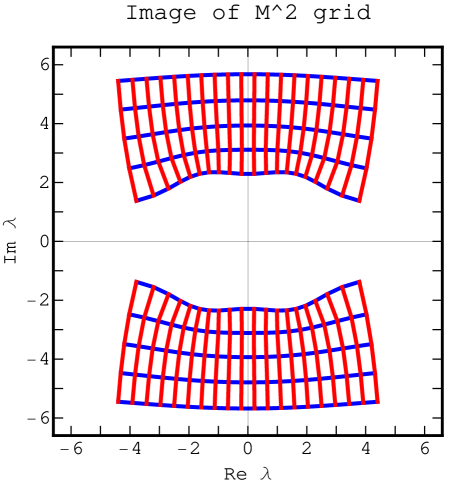
As we reduce , the image of a cartesian grid gets distorted and gaps open near the origin. This illustrated in Fig. 1. The approach of the cut is intricate and involves logarithmic divergences in that we now proceed to study.
III.2 Logarithmic divergences of
For , logarithmic divergences appear in from region of integration where
| (16) |
This only occurs when 0 or . The four cases are = 0 (for (0,0)), 4 (for (0,) or (,0)) and 8 (for . Logarithmic divergences appear when approaches 0, -4 and -8. In order to give a first idea, we have plotted in Fig. 2 the real and imaginary part of when runs over a line slightly above the cut. This figure suggests that the real part has singularities at 0 and -8 and that the imaginary part has singularities at -4.
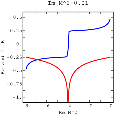
The leading coefficients of the logarithmic singularities can be estimated by using the continuum approximation (16). For instance, if on the real axis, we obtain the familiar relation . For , we have two contributions and by applying the proper Wick rotations, we obtain an imaginary expression that is twice larger in absolute value than the real part near for .
Further insight into the singularities can be obtained by introducing the spectral decomposition :
| (17) |
with
The symmetry (10) implies that
| (19) |
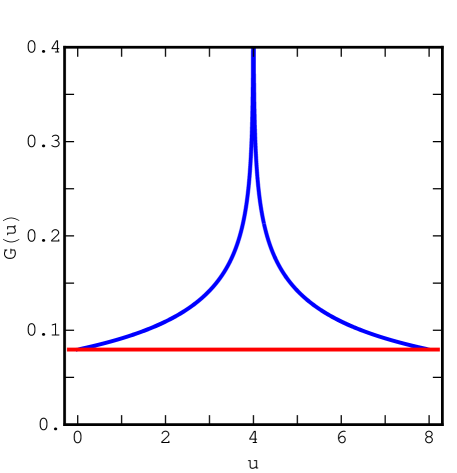
Numerical values for are provided in Fig. 3. The estimate of the singularity of the real part of near implies
| (20) |
which is confirmed numerically in Fig. 3.
From the residue theorem, we find that the imaginary part has a discontinuity along the cut. For ,
| (21) |
From the analysis of the logarithmic singularity of the imaginary part of near , this implies that for ,
| (22) |
This result was confirmed by an analysis of the numerical values of near . Finally, using the fact that when reaches 4, two pairs of inverse square root singularities coalesce into two poles, it is possible to justify that the real part jumps suddenly from -1/4 to 1/4 as increases and crosses -4.
By construction, the integration path in Eq. (17) does not wrap around the pole at . As in the case of the logarithm, we can introduce
| (23) |
which corresponds to have the contour of integration wrapping times around the pole.
III.3 image of the cut plane
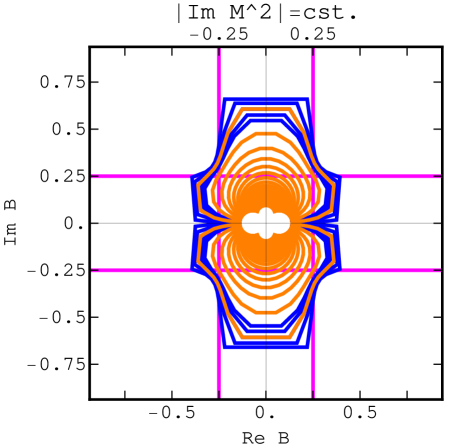
We are now in position to determine the image of the cut plane. The region of large is mapped into a neighborhood of the origin. As we approach the cut, the image of lines of constant imaginary are mapped into hat-shaped curves shown in Fig. 4. In the limit of zero imaginary part, the curves become approximate hyperbolas with asymptotes on the boundary of a cross of width 0.5 centered at the origin. The asymptotes correspond to the logarithmic singularities and can be read from Fig. 2. When has zero real part and a small positive imaginary part, the imaginary part of reaches -0.25 while the real part becomes large and positive. The other asymptote of the approximate hyperbola is reached by approaching -4 from above with a positive imaginary part, the real part of then reaches 0.25 while the imaginary part becomes very negative. All the other cases can be obtained from the symmetry (III).
III.4 image of the cut plane
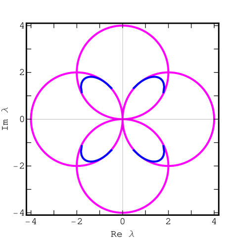
We can now draw more precisely the empty region in the middle of Fig. 1 . Before constructing it, we state the final result: the image of the cut complex plane under the map is the complex plane minus a clover shape centered at the origin and with lobes approximately bisecting the real and imaginary axis. The clover shape shape is visible in Fig. 5.
The boundary of the clover shape is the map of the 4 limiting approximate hyperbolas discussed in the previous subsection. First, we construct the image of the asymptotes. Their images are circles of radius 2 centered at and . Near the origin in the plane, the circles provide a good approximation of the boundary. As we move away from the origin, numerical values are necessary. This is illustrated in Fig. 5.
IV Singularities of
In Sec. III, we have constructed a one-to-one map between the cut plane and the plane with a clover removed. The clover can be filled by adding the images indexed by an integer as defined in Eq. (23). In this Sec., we construct the inverse mapping and discuss its singularities. We start with a simplified example where everything can be done analytically and then discuss the original problem.
IV.1 A simplified example
We will start by constructing the inverse mapping for a simplified mapping for which in the decomposition (17) is constant and equal to . This implies
| (24) |
This modification preserves the logarithmic singularities at 0 and -8 and the symmetry (10). This example is probably closer to what we expect to find for lattice gauge theories. The image of the cut complex plane (fundamental domain) is the horizontal strip bounded by the horizontal lines with imaginary part . The inverse map can be calculated explicitly:
| (25) |
and is invariant under , for any integer . The translated values obtained from the fundamental domain, could be obtained directly by having the path of integration in Eq. (17) wrapping times around . The poles of are located at .
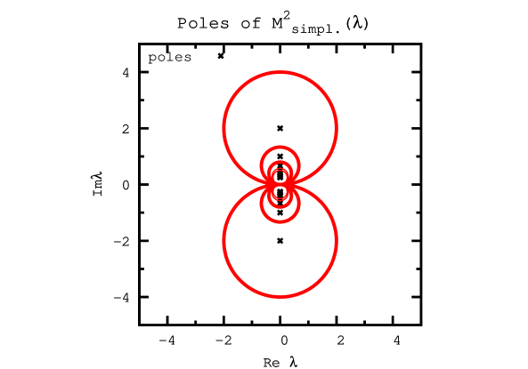
In the plane, the fundamental domain is the complex plane with two circles removed . The boundary of the -translated domains are circles of radius and centered at . The poles are located at . A finite number of boundaries and poles are shown in Fig. 6. For large , the poles and boundaries accumulate at the origin. We believe that some qualitative features of this picture are representative of what is encountered in lattice gauge theory.
IV.2 Qualitative features of
We can now describe qualitatively what happens when we restore the original features of . The fundamental domain in the complex plane becomes strongly distorted when is small as already shown in Fig. 4. The translated domains that were parallel strips in the simplified example are obtained by adding as specified by Eq. (23). The reader can visualize the effect by combining Figs. 4 and 3.
We can now discuss qualitatively the deformation of Fig. 6 that the logarithmic divergence of near imposes. In the plane the strips are pulled at infinity when becomes small. In the plane, the circles are pushed toward the origin along the imaginary axis forming concentric clover shape figures. Importantly, all the poles have moved to the origin.
V The density of states
V.1 Average energy
From the definition of the average energy Eq. (6), we obtain that in the saddle point approximation
| (26) |
Note that and the range is -independent.
When approaches 0 on the positive real axis, approaches zero like . We call the non-perturbative part of . The perturbative expansion terminates at first order. For large , the leading terms cancel and can use the strong coupling expansion (15) to obtain
| (27) |
V.2 Saddle point calculation of
We can use a spectral decomposition of the partition function for all possible energies:
| (28) |
with , the density of state which can be defined as
| (29) |
is non-zero only if in dimensions and this implies that is an analytical function in the entire plane. Using
| (30) |
and varying with respect to (introduced as before) and , we obtain
| (31) |
with and understood as functions of . In these equations is the independent variable and they are equivalent to Eqs. (8) and (26) provided that we identify and . From these results, we obtain
| (32) |
with the entropy density
The duality (5) implies
| (34) |
Numerical values of are shown in Fig. 7. They were calculated using as a parameter first used to fix and from (V.2) and then from Eq. (V.2).
If we rewrite the partition function in terms of the density of states, we obtain the usual thermodynamic relation:
| (35) |
One can check that the saddle point equations imply as expected.
The behavior of can be approximated near the origin. Using and Eq. (35), we obtain
| (36) |
The behavior of near its maximum at can be approximated using Eqs. (27) and (35). The result is
| (37) |
These two approximations fit the numerical values quite well in their region of validity as shown in Fig. 7.
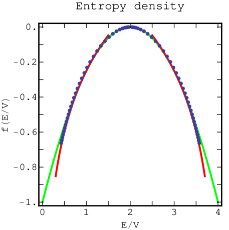
As long as takes values in the real interval , Eq. (35) defines a one-to-one mapping between this interval and the entire real axis. It is clear from Fig. 7 that in this interval and consequently the derivative of the mapping is never zero over the interval. This allows us to integrate over the quadratic fluctuations about the minimum. If an analytical continuation of can be constructed, it seems clear that poles and zeros of will play an important role in the determination of the zeros of the partition function which is the subject of the next section.
VI Zeros of the partition function
There exists a simple relation between the poles of the average energy and the zeros of the partition function. If is a zero of of order , then for . If we now integrate over a closed contour ,
| (38) |
where is the number of zeros of order inside Using Eq. (26), we obtain that in the large limit,
| (39) |
In this expression, is understood as a function of by inverting Eq. (8). The second term has a pole at , but it is compensated by a pole in . This is due to the fact the for small . We now consider possible poles of for other values of . We change variable to write
| (40) |
where is the contour corresponding to in the plane and a short notation for . At finite volume, it is possible write as a ratio of two polynomials. The zeros of the denominator can only be in the cut (the real interval ). This property persists for arbitrarily large volume. Consequently, if the contour in the plane does not cross the cut, then there are no zeros of the partition function inside the corresponding in the -plane. We conclude that in the large- limit, there are no Fisher’s zero in the image of the cut plane. This image has been constructed in Sec. III and limited by four approximate hyperbolas with asymptotes along a cross shaped figure. In the plane, this region becomes the complement of a clover shape figure (see Figs. 4 and 5).
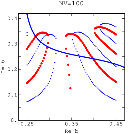
The argument has been checked by numerical calculations using methods similar to those used in lattice gauge theories Denbleyker et al. (2008, 2007). We used spline interpolations from 400 numerical values of in Eq. (V.2) and . In order to remove fast oscillations, we have subtracted the average value of the energy at from in the exponential. This does not affect the complex zeros. The results are shown in Fig. 8 for a rectangle with 0.1 on each side of and (beyond that new methods need to be developed to calculate the rapidly oscillating integrals). The Fisher’s complex zeros are the three isolated points at which the zeros of the imaginary part of meet those of the real part. The image of a line slightly below the cut ( =-0.05) is also shown. As predicted there are no Fisher’s zeros below the image of this line.
The construction points out a relationship between Fisher’s zeros and the poles of . This derivative also appears in the -function
| (41) |
assuming with the renormalized mass kept fixed and the UV cutoff. In the approximation where , we recover the well-known continuum result . Following the finite volume reasoning used above, we see that the poles are exactly cancelled by zeros of . The zeros of the beta function can be interpreted as the singular points of the map which have nontrivial locations at finite volume.
VII Toward a dispersive approach
In quantum mechanics or linear scalar models with a interactions, it is common Bender and Wu (1969, 1973); LeGuillou and Zinn-Justin (1990) to use dispersion relations to estimate the large order behavior of perturbative series. Typically, one considers a quantity, that we will denote , that is analytical in the cut plane with a cut going from to 0. The coefficients of the perturbative series in powers of are then expressed as
| (42) |
For large , the integral is dominated by small negative values of and one can use semi-classical methods to estimate in this regime. Typically, which leads to a factorial growth .
We are interested in finding a dispersive representation of as expressed in the leading order Eq. (26). In this approximation, the series terminates and what we would expect to learn from dispersive methods is that , which appears in the second term of , is zero to all order in , when .
In the rest of this section we will study dispersive expressions for defined in Eq. (25). This simplified expression of the mass gap does has a different behavior when approaches 0 along the imaginary axis but it preserves the basic symmetry (10) and it probably has more resemblance with the gauge models. This choice also has the advantage that all the calculations can be done in terms of elementary functions and that the correctness and accuracy of dispersive expressions can be checked easily. We define
| (43) |
where the contour of integration runs counterclockwise along a circle of center and radius smaller than . In the rest of this section, is real and strictly positive. By construction, is the derivative of evaluated at . If is not exactly zero, we can obtain analytical expressions, such as
| (44) |
The calculated that way are even functions of for odd and larger than 1 and odd functions for even and larger than 2. However, since has a discontinuity at 0, and derivatives should also be present if we wish to obtain expressions valid over the whole real axis.
For , can be approximated by a sum of terms of the form , with . These individual terms peak at where their value grow like . When increases, there is an intermediate region where many large terms cancel and it is difficult to evaluate the function numerically. For instance, for = 12, some numerical noise becomes visible for when 16 digit arithmetic is used.
For , the contribution of the circle at infinity vanishes, and we can deform the contour in Eq. (43) into a clockwise contour encircling the poles on the imaginary axis. Due to the absence of cut or poles on negative real axis, the contribution of two line integrals running on opposite directions along the negative axis cancel. This is contrast to what happens for quantum mechanics and linear scalar models, where there is a discontinuity. Using the residue theorem, we obtain
| (45) |
This expression provides reasonably accurate expressions with truncated sums when is not too small. When becomes small, the sum can be divided into two parts, one with and the other with the rest of the terms. Each sum is of order and the two large sums must cancel to yield an exponentially small results.
Another option is to start with the deformed contour encircling the poles on the imaginary axis keeping it slightly outside of the figure 8 visible on Fig. 6. Changing variable to , this contour is then mapped into a contour encircling the cut from -8 to 0 (but not not containing ). With this contour, we have
| (46) |
with a short notation for given in Eq. (24) and its derivative. The contour can be constructed as a “barbell” figure with three part that we call A, B and C: two lines running along the cut in opposite directions (part A) and two circles going around -8 (part B) and 0 (part C) and stopping when they meet the horizontal lines. We have monitored the contributions of the three parts for and values of and compared them to reliable numerical values of the derivatives of . For small, but not too small values of , A and B provide same sign contributions that dominate the integral. As decreases, the A and B contributions become large and of opposite sign while C becomes negligible. As keeps decreasing, the absolute values of A and B keep increasing until the accuracy of the integrals deteriorate. The situation is illustrated for in Table 1. Again, we are facing the challenge of having two large canceling quantities. We have tried to improve this situation by modifying the radius of the circles and the distance between the horizontal lines, but the general features seem quite persistent.
| T = | A/T | B/T | C/T | |
|---|---|---|---|---|
| 2.0 | -0.00116908 | -0.166729 | 0.536511 | 0.630219 |
| 1.9 | -0.00202112 | 0.257416 | 0.37977 | 0.362814 |
| 1.8 | -0.00296429 | 0.441387 | 0.320456 | 0.238158 |
| 1.7 | -0.00389598 | 0.527325 | 0.305554 | 0.167121 |
| 1.6 | -0.00465005 | 0.552561 | 0.325353 | 0.122087 |
| 1.5 | -0.0049979 | 0.517248 | 0.390845 | 0.0919072 |
| 1.4 | -0.00467868 | 0.379432 | 0.548854 | 0.0717137 |
| 1.3 | -0.00347855 | -0.0515184 | 0.99067 | 0.0608484 |
| 1.2 | -0.0013698 | -2.53523 | 3.45779 | 0.0774331 |
| 1.1 | 0.00131813 | 6.10486 | -5.07936 | -0.0255078 |
| 1.0 | 0.00380812 | 3.56912 | -2.56953 | 0.000410349 |
| 0.9 | 0.00507521 | 3.93213 | -2.93389 | 0.00175748 |
| 0.8 | 0.00449056 | 6.30264 | -5.30373 | 0.0010864 |
| 0.7 | 0.00257563 | 16.7544 | -15.7548 | 0.000454331 |
| 0.6 | 0.000812222 | 93.4553 | -92.4554 | 0.000131085 |
| 0.5 | 0.0000987024 | 1576.99 | -1576.15 | 0.0000229591 |
The lesson that can be learned from the second representation is that the contributions from small negative coupling, which becomes the integral around a cut circle around (part B) after the change of variable, is essential to compensate the large contributions from the cut.
VIII Conclusions
In summary, for nonlinear sigma models, the exact discontinuity of the average energy appears to be a purely non-perturbative phenomenon. At leading order in the expansion the series terminates and no pathological behavior at negative coupling can be inferred from it. It would interesting to see if this feature persists for sub-leading corrections.
In the large- and large volume limit, the Fisher’s zeros can only appear inside a clover shape in the complex plane. It is plausible that as the volume increases, the zeros become dense at the boundary of the clover shape and at the boundary of an infinite set of concentric clover shapes. If this is correct, the zeros closest to the real axis in the plane appear at infinite and . Numerical studies at finite and should clarify the picture and could be used as a guide for the search of Fisher’s zeros in gauge theories. It would also be interesting to consider the case , where there is a rich phase diagram Bardeen et al. (1984); David et al. (1984); Kessler and Neuberger (1985) and where we expect the zeros to pinch the real axis in the infinite volume limit.
A simplified form of the discontinuity was approached with dispersive methods. An important feature observed was that large contributions cancelled. Again, finite volume studies may clarify the mechanism. If we extend the reasoning used for one plaquette Meurice (2006), non perturbative effects become important at an order . Near this order, the coefficients become different if we integrate a perturbative expansion of the density of state from 0 to or from 0 to . This understanding is crucial if we want to modify the weak coupling expansion in order to include non-perturbative effects.
We have noticed that the zeros of the function are related to the singular points of the mapping . At finite volume, these singular points have a nonzero imaginary part. This should be seen as an encouragement to study complexified renormalization group flows as also suggested by other work Polyakov (2004); Kaplan et al. (2009).
Acknowledgements.
We thank C. Bender, D. Du, H. Sonoda and H. Zou for discussions and encouragement. This work was initially motivated by the workshop “New frontiers in large-N gauge theories” where some preliminary results were presented. We thank the organizers and participants for stimulating discussions. The manuscript was written in part while at the Aspen Center for Physics in June 2009. This research was supported in part by the Department of Energy under Contract No. FG02-91ER40664.References
- Dyson (1952) F. Dyson, Phys. Rev. 85, 631 (1952).
- Bender and Wu (1969) C. Bender and T. T. Wu, Phys. Rev. 184, 1231 (1969).
- Bender and Wu (1973) C. M. Bender and T. T. Wu, Phys. Rev. D7, 1620 (1973).
- LeGuillou and Zinn-Justin (1990) J. C. LeGuillou and J. Zinn-Justin, Large-Order Behavior of Perturbation Theory (North Holland, Amsterdam, 1990).
- Pernice and Oleaga (1998) S. Pernice and G. Oleaga, Phys. Rev. D 57, 1144 (1998).
- Meurice (2002) Y. Meurice, Phys. Rev. Lett. 88, 141601 (2002), eprint hep-th/0103134.
- Li and Meurice (2005a) L. Li and Y. Meurice, Phys. Rev. D 71, 016008 (2005a), eprint hep-lat/0410029.
- Di Renzo and Scorzato (2001) F. Di Renzo and L. Scorzato, JHEP 10, 038 (2001), eprint hep-lat/0011067.
- Rakow (2006) P. E. L. Rakow, PoS LAT2005, 284 (2006), eprint hep-lat/0510046.
- Li and Meurice (2005b) L. Li and Y. Meurice, Phys. Rev. D71, 054509 (2005b), eprint hep-lat/0501023.
- Meurice (2006) Y. Meurice, Phys. Rev. D74, 096005 (2006), eprint hep-lat/0609005.
- Denbleyker et al. (2008) A. Denbleyker, D. Du, Y. Liu, Y. Meurice, and A. Velytsky, Phys. Rev. D78, 054503 (2008), eprint 0807.0185.
- Denbleyker et al. (2007) A. Denbleyker, D. Du, Y. Meurice, and A. Velytsky, Phys. Rev. D76, 116002 (2007), eprint arXiv:0708.0438 [hep-lat].
- Li and Meurice (2006) L. Li and Y. Meurice, Phys. Rev. D73, 036006 (2006), eprint hep-lat/0507034.
- Polyakov (2004) A. M. Polyakov, Mod. Phys. Lett. A19, 1649 (2004), eprint hep-th/0405106.
- Novikov et al. (1984) V. A. Novikov, M. A. Shifman, A. I. Vainshtein, and V. I. Zakharov, Phys. Rept. 116, 103 (1984).
- David et al. (1984) F. David, D. A. Kessler, and H. Neuberger, Phys. Rev. Lett. 53, 2071 (1984).
- Polyakov (1987) A. M. Polyakov, Gauge Fields and Strings (Harwood, Chur, Switzerland, 1987).
- Bardeen et al. (1984) W. A. Bardeen, M. Moshe, and M. Bander, Phys. Rev. Lett. 52, 1188 (1984).
- Kessler and Neuberger (1985) D. A. Kessler and H. Neuberger, Phys. Lett. B157, 416 (1985).
- Kaplan et al. (2009) D. B. Kaplan, J.-W. Lee, D. T. Son, and M. A. Stephanov (2009), eprint 0905.4752.