Measuring the History of Cosmic Reionization using the 21-cm PDF from Simulations

Abstract

The 21-cm PDF (i.e., distribution of pixel brightness temperatures) is expected to be highly non-Gaussian during reionization and to provide important information on the distribution of density and ionization. We measure the 21-cm PDF as a function of redshift in a large simulation of cosmic reionization and propose a simple empirical fit. Guided by the simulated PDF, we then carry out a maximum likelihood analysis of the ability of upcoming experiments to measure the shape of the 21-cm PDF and derive from it the cosmic reionization history. Under the strongest assumptions, we find that upcoming experiments can measure the reionization history in the mid to late stages of reionization to $1-10\%$ accuracy. Under a more flexible approach that allows for four free parameters at each redshift, a similar accuracy requires the lower noise levels of second-generation 21-cm experiments.

1 Introduction

The earliest generations of stars are thought to have transformed the universe from darkness to light and to have reionized and heated the intergalactic medium (Barkana & Loeb, 2001). Knowing how the reionization process happened is a primary goal of cosmologists, because this would tell us when the early stars formed and in what kinds of galaxies. The clustering of these galaxies is particularly interesting since it is driven by large-scale density fluctuations in the dark matter (Barkana & Loeb, 2004). While the distribution of neutral hydrogen during reionization can in principle be measured from maps of 21-cm emission by neutral hydrogen, upcoming experiments are expected to be able to detect ionization fluctuations only statistically (for reviews see, e.g., Furlanetto et al., 2006; Barkana & Loeb, 2007). Current observational efforts include the Murchison Widefield Array (MWA, www.haystack.mit.edu/ast/arrays/mwa/), the Low Frequency Array (www.lofar.org), the Giant Metrewave Radio Telescope (gmrt.ncra.tifr.res.in), and the Precision Array to Probe the Epoch of Reionization (astro.berkeley.edu/$\sim$dbacker/eor/).

Studies of statistics of the 21-cm fluctuations have focused on the two-point correlation function (or power spectrum) of the 21-cm brightness temperature. This is true both for analytical and numerical studies and analyses of the expected sensitivity of the new experiments (Bowman, Morales, & Hewitt, 2006; McQuinn et al., 2006). The power spectrum is the natural statistic at very high redshifts, as it contains all the available statistical information as long as Gaussian primordial density fluctuations drive the 21-cm fluctuations. More generally, the power spectrum is also closely related to the directly observed radio visibilities. Now, during reionization the hydrogen distribution is a highly non-linear function of the distribution of the underlying ionizing sources. This follows most simply from the fact that the H I fraction is constrained to vary between 0 and 1, and this range is fully covered in any scenario driven by stars, in which the intergalactic medium is sharply divided between H I and H II regions. The resulting non-Gaussianity (Bharadwaj & Ali, 2005) raises the possibility of using complementary statistics to measuring additional information that is not directly derivable from the power spectrum (e.g., Furlanetto et al., 2004; Saiyad-Ali et al., 2006).

Numerical simulations have recently begun to reach the large scales (of order 100 Mpc) needed to capture the evolution of the intergalactic medium (IGM) during reionization (Iliev et al., 2006b; Mellema et al., 2006b; Zahn et al., 2007; Santos et al., 2008). These simulations account accurately for gravitational evolution and the radiative transfer of ionizing photons, but still crudely for gas dynamics and star formation. Analytically, Furlanetto et al. (2004) used the statistics of a random walk with a linear barrier to model the H II bubble size distribution during the reionization epoch. Schematic approximations were developed for the two-point correlation function (Furlanetto et al., 2004; McQuinn et al., 2005), but recently Barkana (2007) developed an accurate, self-consistent analytical expression for the full two-point distribution within the Furlanetto et al. (2004) model, and in particular used it to calculate the 21-cm correlation function.

Noting the expected non-Gaussianity and the importance of additional statistics, Furlanetto et al. (2004) also calculated the one-point probability distribution function (PDF) of the 21-cm brightness temperature at a point. The PDF has begun to be explored in numerical simulations as well (Ciardi & Madau, 2003; Mellema et al., 2006b). Some of the additional information available in the PDF can be captured by its skewness (Wyithe & Morales, 2007; Harker et al., 2009). Barkana & Loeb (2008) have also considered the difference PDF, a two-dimensional function that generalizes both the one-point PDF and the correlation function and yields additional information beyond those statistics.

Recently, Oh et al. (2009) have quantitatively considered the ability of upcoming experiments to determine the cosmic reionization history from maximum likelihood fitting of the 21-cm PDF. They specifically used mixture modeling of the PDF. In this paper we develop a method for statistical analysis of the PDF that is simpler and more efficient (allowing, in particular, binning of the PDF). We use our method to present a quantitative analysis of whether upcoming and future experiments can measure the detailed shape of the 21-cm PDF and derive from it the cosmic reionization history. In section 2 we develop our basic statistical method for fitting the 21-cm PDF, and test it on a simple toy model for the PDF. We then measure and follow the evolution of the PDF in a large N-body and radiative transfer simulation of cosmic reionization; since previous analytical models of the PDF differ qualitatively from the PDF in the simulation, here we simply fit the simulated PDF with an empirical, four-parameter model (section 3). Finally, we present the expected accuracy of reconstructing the 21-cm PDF and the cosmic reionization history based on the simulated PDF, either with strict assumptions that lead to one free parameter at each redshift (section 4), or with a more flexible approach that allows for four free parameters (section 5). We summarize our conclusions in section 6.

2 Basic Method

In this section we develop our basic statistical method for fitting the PDF. While the statistical approach is general, for concreteness we develop it within the context of a simple toy model for the PDF. We also use this toy, double-Gaussian model in order to get a crude quantitative intuition on how hard it is to measure the 21-cm PDF. We note that we follow to some degree Oh et al. (2009), who considered such a double-Gaussian toy model and made a signal-to-noise study of this model with their analysis method.

2.1 A Toy Model for the PDF

It is useful to have a simple PDF example on which to develop and test our methods. We present here a simplified toy model that captures the main qualitative features of the PDF as seen in the simulations (and shown later in the paper) during the central stage of reionization, when the cosmic ionization fraction $\bar{x}_{i}\sim 0.3-0.6$. The PDF at this stage has a sharp peak at a differential brightness temperature (defined as the difference between the actual brightness temperature and the temperature of the cosmic microwave background at the same frequency) of $T_{b}=0$ mK corresponding to fully ionized pixels, and another peak at $T_{b}\sim 20$ mK corresponding to mostly neutral pixels, with a rapidly declining probability at values above 20 mK, and a smooth probability density in between the peaks that is lower than the height of either peak. In the observations, this physical PDF is convolved with a broad Gaussian corresponding to the thermal noise, resulting in both positive and negative values of $T_{b}$. In the limit when we approximate both peaks as delta functions and neglect the physical PDF at other points, the observed PDF becomes a sum of two Gaussians with equal standard deviations $\sigma$. While certainly highly simplified, this model does capture the main question (relevant especially for low signal-to-noise data, i.e., when $\sigma\gg 20$ mK) of whether it is at all possible to tell apart the two peaks and not confuse them with a convolved single peak (i.e., a single Gaussian).

Thus, we consider two Gaussian distributions with equal standard deviation $\sigma$ (where $\sigma$ represents the measurement noise level). In the toy model we use a dimensionless $s$ as the dependent variable (which represents $T_{b}$ in the real PDF). The Gaussian representing the reionized pixels is centered at $s=0$, while the neutral pixels are represented by a Gaussian centered at $s=s_{G}$. The fraction of the total probability contained in the first Gaussian is $\alpha$. The total distribution is therefore

$$p(s)=\alpha G(s,\sigma)+(1-\alpha)G(s-s_{G},\sigma)\ ,$$ (1)

where

$$G(x,\sigma)\equiv\frac{1}{\sqrt{2\pi}\sigma}\exp(-x^{2}/2\sigma^{2})\ .$$ (2)

Since in the real case only differences in $T_{b}$ can be measured, and not the absolute $T_{b}$ (which is dominated by foregrounds), in the toy model we assume that the absolute $s$ cannot be measured. A simple practical way to do this is to always measure $s$ with respect to its average value according to the PDF of $s$; we do this separately in each model and in each simulated data set, and thus only compare the relative distributions between each model and each data set.

2.2 Maximum Likelihood and the $C$-Statistic

In this subsection we develop our basic statistical method for fitting the PDF, referring to the above toy model as an example for the PDF. In general, we can create mock data sets by randomly generating $N_{p}$ values of $s$ from a given $p(s)$ distribution, and we can then try to estimate the best-fitting parameters with a maximum likelihood method. For a given mock observed PDF, as given by the $N_{p}$ generated values of $s$, we wish to find the best-fitting model PDF $p(s)$ by maximizing the likelihood $\mathcal{L}$ that the $N_{p}$ values $s_{i}$ ($i=1$, 2, $\ldots,$ $N_{p}$) came from $p(s)$. Since the different values $s_{i}$ are independent, this probability (apart from fixed $\Delta s$ factors) is simply

$$\mathcal{L}=\prod_{i=1}^{N_{p}}p(s_{i})\ .$$ (3)

Now, it is standard to replace the problem of maximizing the likelihood $\mathcal{L}$ with a minimization of $-2\ln\mathcal{L}$, which in this case is

$$-2\ln\mathcal{L}=-2\sum_{i=1}^{N_{p}}\ln p(s_{i})\ .$$ (4)

In comparing the data to a potential model, we bin the values of $s$ in order to have a manageable number of bins ($N_{B}=1000$) even when $N_{p}$ is very large. This is justified as long as the bin width is much smaller than any $s$-scale that we hope to resolve in the PDF. We have explicitly checked that using $N_{B}=1000$ bins (with the $C$-statistic, see below) gives the same results as applying equation (4) directly, even for the largest values of $N_{p}$ that we use in this paper. Now, when the expected (according to a model $p(s)$) number of points $n_{{\rm exp},j}$ in each bin $j$ is large (i.e., $n_{{\rm exp},j}\gg 1$), the actual number $n_{j}$ has a standard error of $\sqrt{n_{{\rm exp},j}}$, and we can find the best-fitting model by minimizing a standard $\chi^{2}$ statistic:

$$\chi^{2}=\sum_{j=1}^{N_{B}}\frac{(n_{j}-n_{{\rm exp},j})^{2}}{n_{{\rm exp},j}}\ .$$ (5)

However, in modeling the PDF we often wish to include a wide range of $s$, including some bins where the model probability density $p(s)$ is very low. When $n_{{\rm exp},j}$ is small, the $\chi^{2}$ distribution with its assumption of a Gaussian distribution for each $n_{j}$ severely underestimates the fluctuations in $n_{j}$ compared to the correct Poisson distribution. Thus, equation (5) can lead to major errors if $n_{{\rm exp},j}\ll 1$ in any bin. In this situation, the correct statistic to use is the $C$-statistic (Cash, 1979), derived from the Poisson distribution just as the $\chi^{2}$ statistic is derived from the Gaussian distribution. The $C$-statistic is defined as

$$C=2\sum_{j=1}^{N_{B}}\left(n_{{\rm exp},j}-n_{j}\ln n_{{\rm exp},j}\right)\ .$$ (6)

Note that the Poisson distribution also has a factor of $n_{j}!$ in the denominator, which results in an additional $\ln n_{j}!$ term within the sum in equation (6), but this term does not depend on the model parameters (which enter only through $n_{{\rm exp},j}$) and can thus be dropped from the minimization.

2.3 Results for the Toy Model

For the toy, double-Gaussian model, the parameters we wish to fit to mock data sets are $s_{G}$ and $\alpha$. Note that we assume that $\sigma$ is known, as we expect that the level of thermal noise per pixel will be known in the 21-cm experiments, given the known array properties and the measured foreground level. We perform 1000 Monte Carlo for each input model, and thus obtain the full distribution of reconstructed model parameters. In order to develop intuition on how hard it is to measure the PDF, we define a parameter $\eta$ that captures a simplistic notion of the total signal-to-noise ratio:

$$\eta\equiv\left(\frac{s_{G}}{\sigma}\right)\sqrt{N_{p}}\ ,$$ (7)

motivated by $s_{G}$ as a measure for the signal and $\sigma/\sqrt{N_{p}}$ as a measure for the effective noise after $N_{p}$ measurements with noise $\sigma$ in each. Of course, the ability to detect the two separate peaks also depends on $\alpha$, in that values close to 0 or 1 make one of the peaks insignificant. For a fixed $\alpha$, though, we might naively expect that the accuracy of the reconstructed values of $s_{G}$ and $\alpha$ would not change with the input value of $s_{G}$, as long as we change $N_{p}$ so as to keep the combination $\eta$ fixed.

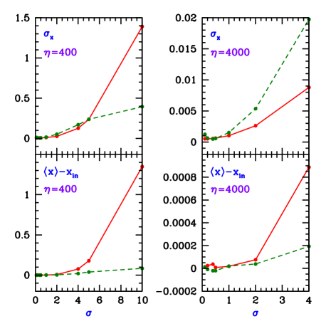
To test this, we fix the input $\alpha=0.4$ and $s_{G}=1$, and vary $\sigma$ and $N_{p}$ together so as to keep $\eta$ fixed. We test $\eta=400$ and 4000, values comparable to those expected in the real experiments discussed later in the paper. The Monte Carlo results are summarized in Figure 1. The results show that the parameters can be accurately reconstructed as long as the signal-to-noise per sample (or per pixel in real data) $s_{G}/\sigma>1$. As long as this is the case, the relative error in $s_{G}$ and $\alpha$ is no worse than $4\%$ ($\eta=400$) or $0.4\%$ ($\eta=4000$), and the average reconstructed values are essentially unbiased. However, once $s_{G}/\sigma$ drops below unity (i.e., $\sigma>1$ in this particular case), the errors increase rapidly with $\sigma$, so that for $\eta=400$ reconstruction is impossible when $\sigma=10$ (i.e., both the bias and spread are of order unity) , and for $\eta=4000$ the errors increase when $\sigma=4$ to a $5\%$ relative spread in $\alpha$.

Figure 1: For each model parameter $x$ reconstructed in each Monte Carlo trial, we show the bias in the average (i.e., the ensemble average $\langle x\rangle$ minus the input value $x_{\rm in}$) and the standard deviation $\sigma_{x}=\sqrt{\langle x^{2}\rangle-\langle x\rangle^{2}}$. We consider the model parameters $s_{G}$ (solid curves, input value 1) and $\alpha$ (dashed curves, input value 0.4), as a function of the noise level (i.e., width of each Gaussian) $\sigma$, where $\eta$ is held fixed at 400 (left panels) or 4000 (right panels).

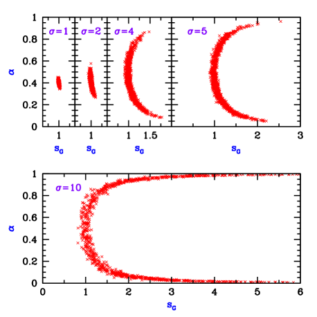
The reason for these increasing errors is parameter degeneracy, as illustrated in Figure 2 for $\eta=400$. While for $\sigma=1$ the reconstructed parameter distribution is fairly symmetrical about the input values of $s_{G}$ and $\alpha$, resembling a standard error ellipse, larger $\sigma$ values produce a stretched error contour that displays a clear (partial) degeneracy between the parameters $s_{G}$ and $\alpha$. Intuitively, when $s_{G}/\sigma\ll 1$ the PDF consists of a narrow input signal (two peaks separated by $s_{G}$, in the case of the toy model) convolved with a broad Gaussian of width $\sigma$. The result is a broad Gaussian of width $\sigma$, with small bumps (distortions). Apparently these small bumps can be produced with very different parameter combinations, resulting in a degeneracy that leads to a large uncertainty when fitting models. While we have considered here a simple toy model, a similar degeneracy is encountered with the real 21-cm PDF, as discussed below.

Figure 2: Distribution of reconstructed model parameters $s_{G}$ and $\alpha$ in 1000 Monte Carlo simulations. The input parameter values are $s_{G}=1$ and $\alpha=0.4$. We vary $\sigma$ keeping $\eta=400$ fixed, so that the number of samples is $N_{p}=160,000\,\sigma^{2}$. Different panels cover different $x$ ranges, but all $x$ axes are shown on the same scale for easy comparison. In the $\sigma\leq 2$ panels, small tick marks are at 0.75 and 1.25.

3 The 21-cm PDF in Simulations

3.1 Numerical Simulation

In this paper we utilize a large-scale N-body and radiative transfer simulation of cosmic reionization following the methodology first presented in Iliev et al. (2006b). The cosmological structure formation and evolution is followed with a particle-mesh N-body code called PMFAST (Merz et al., 2005). These N-body results then provide the evolving density field of the IGM, as well as the location and mass of all the halo sources, as input to a separate radiative transfer simulation of inhomogeneous reionization. The latter is performed with the ${\rm C}^{2}-$Ray (Conservative, Causal Ray-Tracing) code, a regular-grid, ray-tracing, radiative transfer and nonequilibrium chemistry code (Mellema et al., 2006a). The ionizing radiation is ray-traced from every source cell to every grid cell at a given timestep using a method of short characteristics. ${\rm C}^{2}-$Ray is designed to be explicitly photon-conserving in both space and time, which ensures an accurate tracking of ionization fronts, independently of the spatial and time resolution. This is true even for grid cells which are very optically thick to ionizing photons and time steps long compared to the ionization time of the atoms, which results in high efficiency. The code has been tested against analytical solutions (Mellema et al., 2006a), and directly compared with other radiative transfer methods on a standardized set of benchmark problems (Iliev et al., 2006a, 2009).

We simulated the $\Lambda$CDM universe with $1624^{3}$ dark matter particles of mass $2.2\times 10^{7}\,{\rm M}_{\odot}$, in a comoving simulation volume of $(100\,h^{-1}\,{\rm Mpc})^{3}$. This allowed us to resolve (with 100 particles or more per halo) all halos of mass $2.2\times 10^{9}\,{\rm M}_{\odot}$ and above. The radiative transfer grid has $203^{3}$ cells. The H-ionizing photon luminosities per halo in our cosmic reionization simulations are assigned as follows. A halo of mass $M$ is assumed to have converted a mass $M\cdot(\Omega_{b}/\Omega_{m})\cdot f_{*}$ into stars, where $f_{*}$ is the star formation efficiency. Halo catalogs are discrete in time, because N-body density fields are stored every $\Delta t\sim 20\,{\rm Myrs}$ and the corresponding halo catalogs are produced at the same time. If each source forms stars over a period of time $\Delta t$ and each stellar nucleus produces $N_{i}$ ionizing photons per stellar lifetime and is used only once per $\Delta t$, and if a fraction $f_{\rm esc}$ of these photons escape into the IGM, then the ionizing photon number luminosity of a halo of mass $M$ is given by

$$Q_{i}=\frac{N_{i}\cdot f_{{\rm esc}}\cdot f_{*}\cdot M\left(\Omega_{b}/\Omega_{m}\right)}{\Delta t\cdot\mu m_{H}}\ ,$$ (8)

where $m_{H}$ is the mass of a hydrogen atom and $\mu=1.22$ so that $\mu m_{H}$ is the mean mass per nucleus. In this model, stars are produced in a burst, and they keep radiating with a fixed $Q_{i}$ for $\Delta t\simeq 20\,{\rm Myrs}$. We choose here a specific case, first presented (and labeled f250) in Iliev et al. (2007) and further discussed in Iliev et al. (2008). In this scenario, halos are assumed to host relatively low efficiency emitters, with $f_{\gamma}\equiv f_{*}f_{{\rm esc}}N_{{\rm i}}=250$ (corresponding, e.g., to Pop II stars with a Salpeter IMF).

The simulation we use in this work assumes a flat ($\Omega_{k}=0$) $\Lambda$CDM cosmology. The simulation is based on the WMAP 3-year results, which derived the parameters ($\Omega_{m},\Omega_{\Lambda},\Omega_{b},h,\sigma_{8},n)=(0.24,0.76,0.042,0.73,0.74,0.95)$ (Spergel et al., 2007). Here $\Omega_{m}$, $\Omega_{\Lambda}$, and $\Omega_{b}$ are the total matter, vacuum, and baryonic densities in units of the critical density, $\sigma_{8}$ is the root-mean-square density fluctuation on the scale of $8h^{-1}{\rm Mpc}$ linearly extrapolated to the present, and $n$ is the power-law index of the primordial power spectrum of density fluctuations.

3.2 The Simulated 21-cm PDF

During cosmic reionization, we assume that there are sufficient radiation backgrounds of X-rays and of Ly$\alpha$ photons so that the cosmic gas has been heated to well above the cosmic microwave background temperature and the 21-cm level occupations have come into equilibrium with the gas temperature. In this case, the observed 21-cm differential brightness temperature (i.e., relative to the cosmic microwave background) is independent of the spin temperature and, for our assumed cosmological parameters, is given by (Madau et al., 1997)

$$T_{b}=\tilde{T}_{b}\Psi;\ \ \ \ \tilde{T}_{b}=23.7\left(\frac{\Omega_{b}h}{0.032}\right)\sqrt{\left(\frac{0.3}{\Omega_{m}}\right)\left(\frac{1+z}{8}\right)}\,{\rm mK}\ ,$$ (9)

with $\Psi=x^{n}[1+\delta]$, where $x^{n}$ is the neutral hydrogen fraction and $\delta$ is the relative density fluctuation. Under these conditions, the 21-cm fluctuations are thus determined by fluctuations in $\Psi$. We denote the PDF by $p(T_{b})$, normalized so that $\int p(T_{b})dT_{b}=1$.

To calculate the 21-cm PDF, we smooth the 21-cm emission intensity over our full simulation volume with a cubical top-hat filter (sometimes referred to as “boxcar” averaging) of a pre-determined size $R_{\rm pix}$. We then assemble the PDF of the resulting values over a fine grid, much finer than $R_{\rm pix}$. This effectively smooths out the fluctuations in the PDF and yields a smooth function, but we note that there is still a real sample (or “cosmic”) variance limit on the accuracy of our simulated PDF, resulting from the limited number of independent volumes of size $R_{\rm pix}$ within our simulation box. We use $R_{\rm pix}=5\,h^{-1}$ Mpc, $10\,h^{-1}$ Mpc, and $20\,h^{-1}$ Mpc, yielding a number of independent volumes equal to 8000, 1000, and 125, respectively. The analogous results for the first-year WMAP cosmology were previously presented, for a few redshifts only, in Mellema et al. (2006b) (with a similarly-defined ionized fraction PDF shown in Iliev et al. (2006b)).

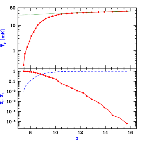
Figure 3 shows the overall progress of reionization as a function of redshift in the simulation. We calculate the PDF at 26 redshifts spanning a global mass-weighted ionization fraction $\bar{x}_{i}$ from $6\times 10^{-6}$ to $99.0\%$, with the cosmic mean 21-cm differential brightness temperature $\bar{T}_{b}$ ranging from 36.5 mK to 0.27 mK. Of course, we assume that $\bar{T}_{b}$ itself is not directly observable, due to the bright foregrounds. The main goal of the PDF analysis is to reconstruct $\bar{x}_{i}$ vs. $z$ using the $T_{b}$ fluctuations as captured in the PDF at each redshift.

Figure 3: The global progress of cosmic reionization in the simulation, as a function of the redshift $z$. Bottom panel: we show the mass-weighted ionized fraction $\bar{x}_{i}$ (solid curve) and the corresponding neutral fraction $\bar{x}_{n}=1-\bar{x}_{i}$ (dashed curve). Top panel: we show the cosmic mean 21-cm differential brightness temperature $\bar{T}_{b}$ in the simulation (solid curve), and the mean $T_{b}$ expected for a neutral universe of uniform density (dotted curve). Also indicated in each panel are the 26 output redshifts used in the analysis below (points).

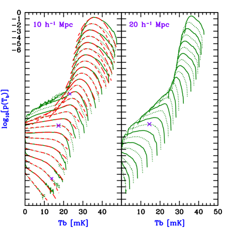
We show the measured simulation PDFs for various redshifts and $R_{\rm pix}=5\,h^{-1}$Mpc in Figure 4. The PDF starts out close to Gaussian at high redshift, when the ionized volume is negligible and the density fluctuations on the scale $R_{\rm pix}$ are fairly linear and thus give a Gaussian PDF. There is also a clear skewness, seen particularly in a high-density tail that drops more slowly with $T_{b}$ than the Gaussian fit (more on the fitting function below); this results from the non-linear growth of density fluctuations.

Figure 4: The 21-cm PDF in 5 $h^{-1}$Mpc cubic pixels, shown versus the differential brightness temperature $T_{b}$. We show $\log_{10}$ of the PDF, which itself is expressed in units of 1/mK. We show the PDF obtained from the simulation (alternating solid and dotted curves) and our best fits to them (alternating long-dashed and short-dashed curves). The 26 redshifts (see Figure 3) range from $z=15.729$ (top) to 7.460 (bottom). The highest-redshift PDF is shown at its actual value, corresponding to the labels at the top of the $y$-axis; each subsequent PDF is shifted vertically down by a factor of 10 in the PDF. The $\times$ mark points (where $T_{b}$ equals the best-fit $T_{L}$) on three simulated PDFs: early in reionization ($z=10.08$, $\bar{x}_{i}=0.156$), right after the midpoint ($z=8.79$, $\bar{x}_{i}=0.530$), and late in reionization ($z=7.75$, $\bar{x}_{i}=0.948$); these points mark the 12-redshift range that is used in the fitting of mock data in the following sections.

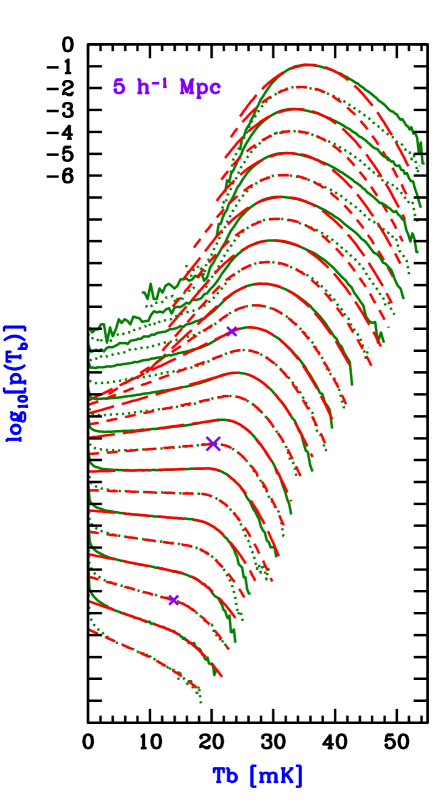
As reionization gets under way, the high-density tail drops off and (coincidentally) approaches the Gaussian shape, as high-density pixels are more likely to be partially or fully ionized and thus have their $T_{b}$ reduced. When $\bar{x}_{i}$ reaches a fraction of a percent, the still fairly Gaussian PDF develops a significant low-$T_{b}$ tail which is roughly exponential (i.e., linear in the plot of log of the PDF). This tail corresponds to pixels that are substantially ionized, i.e., where a large fraction of the pixel volume partially overlaps one or more ionized bubbles. Soon afterward, a significant peak can be seen near $T_{b}=0$ mK, corresponding to fully ionized pixels (i.e., pixels in which the hydrogen in the IGM has been fully ionized, but there may remain a small bit of high-density neutral gas). Near the mid-point of reionization ($\bar{x}_{i}=50\%$), there is still a half-Gaussian peak (at $T_{b}\sim 20$ mK), i.e., with a Gaussian drop-off towards higher $T_{b}$, now with a nearly flat exponential tail towards lower $T_{b}$, and a prominent peak at $T_{b}=0$ mK. The peak at zero increasingly dominates towards the end of reionization, as most pixels become fully ionized, but there remains an exponential tail out to higher $T_{b}$, with a cutoff (at $T_{b}\sim 20$ mK).

The PDFs are shown for $R_{\rm pix}=10\,h^{-1}$Mpc and $20\,h^{-1}$Mpc in Figure 5. The qualitative evolution of the PDF throughout reionization is similar to the $R_{\rm pix}=5\,h^{-1}$Mpc case, but the PDF is narrower for larger $R_{\rm pix}$ since the 21-cm fluctuations are smaller when smoothed on larger scales. Also, for larger $R_{\rm pix}$ there are fewer pixels in the peak near $T_{b}=0$ mK since it is more difficult to fully ionize large pixels. The PDFs for $R_{\rm pix}=20\,h^{-1}$Mpc are not so reliable, as they are measured based on only 125 independent volumes. Also, their shapes differ significantly from the PDFs in the smaller pixels, and so they cannot be successfully fitted with the same model used for the other PDFs. Thus, in this paper we focus on the two smaller values of $R_{\rm pix}$ and only present fits to the corresponding PDFs. Observations of the PDF are most promising during the central stage of reionization, when the PDF has two significant, well-separated peaks rather than a single narrow peak (as is the case either very early or very late in reionization). This two-peak regime covers $\bar{x}_{i}\sim 30-90\%$ for $R_{\rm pix}=5\,h^{-1}$Mpc, but only $\bar{x}_{i}\sim 75-95\%$ for $R_{\rm pix}=10\,h^{-1}$Mpc, because of the rarity of fully ionized pixels in the latter case. However, even without a strong peak at zero, the extended nearly flat (exponential) part of the PDF during reionization helps in measuring the PDF, as we find below.

Figure 5: Same as Figure 4 but for cubic pixels of size 10 $h^{-1}$Mpc (left panel) or 20 $h^{-1}$Mpc (right panel). In the right panel we show only the simulated PDFs, and the $\times$ marks the peak of the PDF right after the midpoint of reionization ($z=8.79$).

3.3 The GED Model Fit to the Simulated PDF

Previous analytical models of the PDF do not describe our simulated PDFs well. While the Gaussian at high redshift and the $T_{b}=0$ mK Delta function at the end of reionization are obvious, the precise shape at intermediate redshifts seems to depend on the precise topology of the ionized bubbles and the geometry of their overlap with the cubic pixels. Here we take an empirical approach based on our numerical simulation. Thus we use a Gaussian + Exponential + Delta function (GED) model for the PDF $p(T_{b})$. The Dirac Delta function is centered at zero, and is connected with an exponential to the Gaussian. The model depends on four independent parameters: $T_{G}$ (center of Gaussian), $\sigma_{G}$ (width of Gaussian), $c_{G}$ (height of Gaussian peak) and $T_{L}$ (transition point between the exponential and the Gaussian). Our GED model is thus:

$$p(T_{b})=\cases{p_{1}(T_{b})=P_{D}\delta_{D}(T_{b})+a\,\exp(\lambda T_{b})\ ,&$0\leq T_{b}\leq T_{L}$\cr p_{2}(T_{b})=\displaystyle{c_{G}\exp\left[-\frac{(T_{b}-T_{G})^{2}}{2\,\sigma_{G}^{2}}\right]}\ ,&$T_{b}>T_{L}$\cr}$$ (10)

where $\delta_{D}(x)$ is the Dirac delta function. The quantities $a$ and $\lambda$ can be expressed in terms of the above four parameters by requiring the exponential and Gaussian functions to connect smoothly at $T_{b}=T_{L}$. The conditions $p_{1}(T_{L})=p_{2}(T_{L})$ and $p_{1}^{\prime}(T_{L})=p_{2}^{\prime}(T_{L})$ lead to

$$\lambda = \frac{T_{G}-T_{L}}{\sigma_{G}^{2}}\ ,$$ (11)

$$a = c_{G}\exp\left[-\frac{(T_{L}-T_{G})^{2}}{2\,\sigma_{G}^{2}}-\lambda T_{L}\right]\ .$$ (12)

Also, $P_{D}$ is determined by the requirement of normalization; the total integrated probability is unity if $P_{D}=1-P_{E}-P_{G}$, where

$$P_{E} = \int_{+\epsilon}^{T_{L}}p_{1}(T_{b})dT_{b}=\frac{a}{\lambda}\left[\exp(\lambda T_{L})-1\right]\ ,$$ (13)

$$P_{G} = \int_{T_{L}}^{\infty}p_{2}(T_{b})dT_{b}=c_{G}\sqrt{\frac{\pi}{2}}\sigma_{G}\,{\rm erfc}\left(\frac{T_{L}-T_{G}}{\sqrt{2}\,\sigma_{G}}\right)\ .$$ (14)

Note that the parameters $P_{D}$, $P_{E}$ and $P_{G}$ represent the relative contribution to the total probability from the delta function, the exponential function, and the Gaussian function, respectively.

Using the GED model, we determine the values of $T_{G}$, $\sigma_{G}$, $c_{G}$ and $T_{L}$ as functions of redshift by fitting to the simulation PDFs for pixels of 5 $h^{-1}$Mpc and 10 $h^{-1}$Mpc. In approaching this fitting, we note that we focus on the main features of the PDF, and not on the fine details. In particular, we do not worry about features that contain a small fraction of the total probability, or on the detailed PDF shape on scales finer than several mK. This is justified since the observations are difficult, and most likely will not be sensitive to these fine details, at least in the upcoming 21-cm experiments. In addition, our simulated PDF may not be reliable in its fine details, since we are using a single, limited simulated volume, and more generally, numerical simulations of reionization still lack a detailed demonstration of convergence.

Thus, we do not try to fit the detailed peak shape at $T_{b}=0$, but instead represent the total probability of that region with the Delta function. In practice we only fit to the data beyond the lowest values of $T_{b}$, and then set the Delta function contribution $P_{D}$ to get the correct overall normalization. Specifically, for each PDF we first find $T_{b,h}$ which is the highest value of $T_{b}$ where $p(T_{b,h})>10^{-4}$. We then only fit to the data with $T_{b}>5$ mK, if $T_{b,h}\geq 20$ mK, or to the data with $T_{b}>T_{b,h}/4$, if $T_{b,h}<20$ mK. At redshifts where the simulation data do not have a Delta function feature, i.e., there are no pixels near $T_{b}=0$, we make a fit constrained by setting $P_{D}=1-P_{E}-P_{G}=0$; this is the case at the highest redshifts, namely $z\geq 10.924$ for $R_{\rm pix}=5\,h^{-1}$Mpc and $z\geq 9.034$ for $R_{\rm pix}=10\,h^{-1}$Mpc.

Our GED model fits are shown along with the PDFs in Figs. 4 and 5. The fits are very good during the central and late stages of reionization, except for the detailed shape (which we do not try to fit) of the $T_{b}=0$ peak which extends out to $T_{b}\sim 2-4$ mK. These are the redshifts that we focus on in this paper, and which are most promising to observe. The fits are also quite good at the highest redshifts, where the simulated PDF is essentially Gaussian except for the skewness. This skewness, though, affects mainly the tails of the distribution; e.g., at the highest redshift ($z=15.729$) for $R_{\rm pix}=5\,h^{-1}$Mpc, $\sim 60\%$ of the total probability is contained at $T_{b}$ values above the peak of the PDF, i.e., the high-density tail adds about $10\%$ to the $50\%$ of a symmetrical Gaussian. As noted above, this high-density tail declines with time due to ionization offsetting the high density of overdense pixels. Thus, the high-$T_{b}$ tail becomes well fitted by the Gaussian model once $\bar{x}_{i}$ rises above a few percent. At later times the cutoff becomes somewhat steeper than the Gaussian fit, especially for $R_{\rm pix}=10\,h^{-1}$Mpc, but this only affects the insignificant tail end of the PDF at the highest $T_{b}$. For instance, for $R_{\rm pix}=10\,h^{-1}$Mpc at $\bar{x}_{i}=0.530$, the tail beyond $T_{b}=23$ mK (where the cutoff starts to differ significantly from the fit) contains only $0.2\%$ of the total probability.

Another small mismatch occurs when reionization gets significantly under way but is still fairly early. The transition region from a near-Gaussian to a near-exponential shape is not well-fit at these times by our model, and as a result the fit is significantly below the low-$T_{b}$, roughly linear (exponential) tail. This mismatch is significant in the range of $\bar{x}_{i}$ from a few percent up to $\sim 30\%$, and at these redshifts this exponential tail typically contains only a few percent of the total probability (up to $10\%$).

Figure 6 shows how our model parameters vary as cosmic reionization progresses. The Gaussian peak position $T_{G}$ and height $c_{G}$ both decline with time due to the increasing ionization of even low-density pixels. At least a half-Gaussian is present until $\bar{x}_{i}\sim 60\%$, but after that $T_{L}>T_{G}$ and only the Gaussian cutoff remains. The parameter $\sigma_{G}$ remains at a value of a few mK throughout reionization; it gives a measure of density fluctuations, initially purely and later together with some correlation with ionization. At the very end of reionization, $T_{G}\rightarrow 0$ and then $\sigma_{G}$ and $c_{G}$ lose their usual meaning (e.g., $c_{G}$ becomes an indirect parameterization of the normalization of the exponential portion).

Figure 6: Our best-fitting GED model parameters $T_{G}$ (solid curve), $T_{L}$ (long-dashed curve), $\sigma_{G}$ (short-dashed curve), and $c_{G}$ (dotted curve, different $y$-axis range) as functions of the cosmic mass-weighted ionization fraction. They are obtained by fitting to the simulated PDFs for pixels of size 5 $h^{-1}$Mpc (bottom panel) or 10 $h^{-1}$Mpc (top panel).

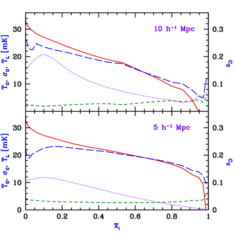
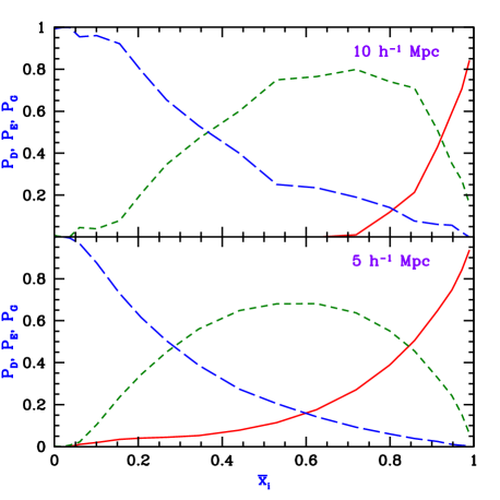
Figure 7 shows the evolution of the probabilities $P_{D}$ (representing the delta function), $P_{E}$ (exponential), and $P_{G}$ (Gaussian), which together add up to unity. The Figure shows how the 21-cm PDF is gradually transformed from a Gaussian to a delta function, with the exponential dominating at intermediate times (mid to late reionization). Note that in the limit of infinite resolution, we would have $P_{D}=\bar{x}_{i}$. With a finite resolution, $P_{D}$ can be thought of as the cosmic ionized fraction smoothed at the observed resolution. In practice, converting observed values of $P_{D}$, $P_{E}$, and $P_{G}$ to the true $\bar{x}_{i}$ requires some modeling.

Figure 7: The derived probabilities $P_{D}$ (solid curve), $P_{E}$ (short-dashed curve) and $P_{G}$ (long-dashed curve) as functions of the cosmic mass-weighted ionization fraction. They are obtained by fitting the GED model to the simulation PDFs for pixels of size 5 $h^{-1}$Mpc (bottom panel) or 10 $h^{-1}$Mpc (top panel).

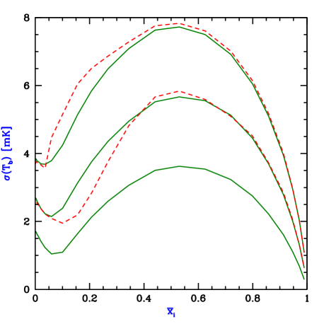
We also calculate the variance $\langle T_{b}^{2}\rangle-\langle T_{b}\rangle^{2}$ from the PDF both directly from the original simulation data and from our GED model fits. We plot this in Figure 8 for two reasons. First, the plot shows that the GED model reproduces the variance of the real PDF rather well, especially where the upcoming measurements are more promising (i.e., later in reionization). Second, the Figure illustrates a symmetry in that the variance is maximum near the midpoint of reionization, and has lower values both before and after the midpoint; this symmetry helps explain a near-degeneracy that we sometimes find below, when we consider low signal-to-noise data for which it is difficult to measure the detailed shape of the PDF, and the variance is a major part of what can be measured.

Figure 8: Standard deviation $\sqrt{\langle T_{b}^{2}\rangle-\langle T_{b}\rangle^{2}}$ as a function of the cosmic mass-weighted ionization fraction. We show this quantity for the original simulation data (solid curves) and from our GED model fits (dashed curves). We consider the PDF in boxes of size 5 $h^{-1}$Mpc, 10 $h^{-1}$Mpc and 20 $h^{-1}$Mpc (top to bottom, only simulation data for the 20 $h^{-1}$Mpc case).

4 Monte-Carlo Results with One Free Parameter

In the rest of this paper, we present results for the expected accuracy of reconstructing the 21-cm PDF itself and the cosmic reionization history from the PDF. To obtain these results, we assume that our simulation accurately reproduces the real reionization process in the universe, and furthermore we assume that our GED model introduced in the previous section can be used as a substitute for the PDF from the simulation. In the future, more realistic simulations and more elaborate PDF fits can be used instead, but the general idea will be the same: as long as the overall signal-to-noise ratio is low, it is essential to rely on simulations in order to both reconstruct and interpret the observed PDF.

Of course, even if simulations perfectly predicted the 21-cm PDF for given inputs, various astrophysical scenarios would give somewhat different ionizing source and sink properties, and might yield a variety of possible PDFs. We leave the detailed exploration of this issue for future work, and here assume that the simulated scenario matches reality, except that a small number of free parameters are allowed to vary and must be reconstructed by trying to match the observed PDF. In this section, we reconstruct reionization from the PDF under the most optimistic assumption, where we assume that the real PDF matches the simulated one as a function of just a single parameter, the ionization fraction $\bar{x}_{i}$. Thus, at each redshift, we find the value of $\bar{x}_{i}$ that best matches the observed PDF, assuming that the PDF varies with $\bar{x}_{i}$ as in the simulation. In practice we expect that $\bar{x}_{i}$ is indeed the main parameter that determines the PDF, but there should be some small additional dependence on redshift and astrophysical inputs. In the next section we explore a more flexible approach which makes much weaker assumptions.

Thus, here we wish to know how well a certain experiment can determine $\bar{x}_{i}$ assuming this one-parameter model. An experiment is specified by a total number of pixels $N_{p}$ and a noise per pixel $\sigma_{N}$. We can simulate an observed PDF from such an experiment at a given input $\bar{x}_{i}$ by generating $N_{p}$ data points from the PDF of equation (10) and adding to each noise generated from a Gaussian distribution with standard deviation $\sigma_{N}$. The resulting Monte-Carlo-generated “observed” PDF is then compared, via the $C$-statistic of equation (6), to the model, which is equation (10) convolved with the Gaussian noise. This convolved function $q(T_{b})$ equals:

$$q(T_{b})=P_{D}\,G(T_{b},\sigma_{N})+q_{1}(T_{b})+q_{2}(T_{b})\ ,$$ (15)

where $G$ is a Gaussian (eq. 2), and

$$q_{1}(T_{b}) = \frac{1}{2}a\exp\left(\frac{\lambda^{2}\sigma_{N}^{2}}{2}+\lambda T_{b}\right)\times$$

$$\left\{{\rm erf}\left(\frac{\lambda\sigma_{N}^{2}+T_{b}}{\sqrt{2}\sigma_{N}}\right)-{\rm erf}\left(\frac{\lambda\sigma_{N}^{2}-T_{L}+T_{b}}{\sqrt{2}\sigma_{N}}\right)\right\}\ ,$$

$$q_{2}(T_{b}) = \frac{1}{2}c_{G}\frac{\sigma_{G}}{\sigma_{c}}\exp\left\{-\frac{(T_{b}-T_{G})^{2}}{2\sigma_{c}^{2}}\right\}\times$$

$${\rm erfc}\left\{\frac{\sigma_{N}^{2}(T_{L}-T_{G})+\sigma_{G}^{2}(T_{L}-T_{b})}{\sqrt{2}\sigma_{c}\sigma_{G}\sigma_{N}}\right\}\ ,$$

where $\sigma_{c}^{2}=\sigma_{G}^{2}+\sigma_{N}^{2}$. As noted above, in this section we regard $q(T_{b})$ as a one-parameter function of $\bar{x}_{i}$, taking $T_{G}$, $\sigma_{G}$, $c_{G}$ and $T_{L}$ to be functions of $\bar{x}_{i}$ as shown in Figure 6. For clarity we denote the input, real cosmic ionized fraction simply $\bar{x}_{i}$, while the free parameter which is the output of the fitting we denote $\bar{x}_{i}^{\rm out}$. Note that we assume that the experimental setup is sufficiently well characterized that $\sigma_{N}$ is known and need not be varied in the fitting. Also note that while the various temperatures we have defined ($T_{b}$, $T_{L}$, and $T_{G}$) refer to the differential brightness temperature (i.e., 0 mK refers to the absence of a cosmological signal), in practice, when the foregrounds as well as the cosmic microwave background are subtracted, the mean cosmological signal on the sky will be removed as well, since there is no easy way to separate out different contributions except through their fluctuations. Thus, as in section 2.1, we assume that the absolute $T_{b}$ cannot be measured, and in our fitting always measure $T_{b}$ with respect to its average value according to the PDF, both in each model and in each simulated data set.

For the experimental specification, we adopt the (rough) expected parameters for one-year observations of a single field of view with the MWA. We use the relations for 21-cm arrays from the review by Furlanetto et al. (2006), adopting a net integration time $t_{\rm int}=1000$ hours, a collecting area $A_{\rm tot}=7\times 10^{3}\ {\rm m}^{2}$, a field of view of $\pi 16^{2}\ {\rm deg}^{2}$, and a total bandwidth $\Delta\nu_{\rm tot}=6$ MHz. Then assuming cubic pixels of comoving size $r_{\rm com}$, we find

$$N_{p} = 6.0\times 10^{6}\,\left(\frac{r_{\rm com}}{5h^{-1}{\rm Mpc}}\right)^{-3}\,\left(\frac{1+z}{10}\right)^{0.9}\ ,$$ (18)

$$\sigma_{N} = 200\left(\frac{r_{\rm com}}{5h^{-1}{\rm Mpc}}\right)^{-2.5}\,\left(\frac{1+z}{10}\right)^{5.25}\,{\rm mK}\ .$$ (19)

In order to explore the dependence on the noise level, we also consider various specifications with lower noise in the same field of view, e.g., 1/2 the noise we denote as MWA/2 (which corresponds, e.g., to four-year data with the MWA), while 1/10 the noise we denote as MWA/10 (which corresponds to the regime of larger, second-generation 21-cm arrays). Note that we include only Gaussian thermal noise, whose magnitude is determined by the receiver’s system temperature, which in turn is set by the sky’s brightness temperature which is dominated by Galactic synchrotron emission (Furlanetto et al., 2006). In particular this assumes perfect foreground removal from the 21-cm maps; we leave an analysis of the effect of foreground residuals for future work.

We note the following conversions between comoving distance and observational units of angular and frequency resolution:

$$5h^{-1}{\rm Mpc}\approx 2.6^{\prime}\,\left(\frac{1+z}{10}\right)^{-0.2}\approx 0.37\,{\rm MHz}\,\left(\frac{1+z}{10}\right)^{-0.5}\ .$$ (20)

The diffraction limit of the MWA is several arcminutes, but its frequency resolution will be around 10 kHz. In principle, this allows a measurement of the PDF in skinny boxes (thinner in the redshift direction) rather than cubes. This would give us more points but with less signal in each, keeping the overall signal-to-noise ratio about the same. By accessing fluctuations on smaller scales, this skinny-box PDF would be somewhat broader than the cubic one but on the other hand, our quantitative results for the toy model above suggest that decreasing the signal-to-noise ratio per pixel in this way would have a strong tendency to introduce partial degeneracies. Thus, we do not expect this option to be productive (except in the cases when the errors in the cubic PDF are very small), and focus here on the simplest case of the 21-cm PDF measured in cubes.

At each redshift, we generate 1000 Monte Carlo instances of observed PDFs and minimize the $C$-statistic to find the best-fitting model in each case. Results for MWA and MWA/2 errors are plotted in Figure 9, which shows that for first-generation experiments the larger (10 $h^{-1}$Mpc) boxes are much more promising, since the lower noise $\sigma_{N}$ (by a factor of $\sim 6$) dominates despite the narrower PDF (compare Figs. 4 and 5) and smaller number of pixels $N_{p}$ (by a factor of 8). We note that lower noise is particularly important in view of the partial degeneracy (demonstrated in section 2.3 for the toy model) that arises when $\sigma_{N}$ is greater than the characteristic width of the intrinsic PDF. The partial degeneracy is also apparent in comparing the MWA and MWA/2 cases, where at some $\bar{x}_{i}$ values, halving the errors crosses a degeneracy threshold and cuts the output uncertainty in a non-linear fashion. We caution that cases that are very near such a threshold may be susceptible to additional numerical errors.

Figure 9: Expected 1$\sigma$ errors on reconstructing the cosmic mean ionized fraction from the PDF, assuming just one free parameter. Specifically, for each input value of $\bar{x}_{i}$ we show the output median (i.e., 50 percentile) $\bar{x}_{i}^{\rm out}$ as well as the 16 to 84 percentile range. We consider MWA 1-yr errors (left panels) or MWA/2 (right panels), for the PDF in 5 $h^{-1}$Mpc boxes (top panels) or 10 $h^{-1}$Mpc boxes (bottom panels).

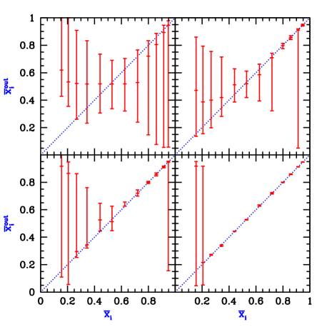
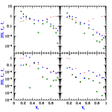
The same results are shown in Figure 10 in terms of relative errors, making it easier to see and compare both small and large errors. Specifically, in terms of the various percentile output ionization fractions (e.g., we denote the median by $\bar{x}_{i}^{\rm out,50}$), we show $f_{0}=(\bar{x}_{i}^{\rm out,50}/\bar{x}_{i})-1$ (the relative difference between the median output value and the true input value, representing the fractional bias of the reconstruction), $f_{+}=(\bar{x}_{i}^{\rm out,84}/\bar{x}_{i}^{\rm out,50})-1$ (the relative difference between the $84\%$ and median values, representive the fractional $+1\sigma$ spread), and $f_{-}=1-(\bar{x}_{i}^{\rm out,16}/\bar{x}_{i}^{\rm out,50})$ (the relative difference between the $16\%$ and median values, representive the fractional $-1\sigma$ spread). The Figure shows that the reconstruction is typically unbiased within the errors (i.e., the $1\sigma$ range is significantly larger than the bias in the median), except for some points in the early stages of reionization. Only a little information is available with the PDF in the smaller boxes (except for a few redshifts with MWA/2 errors); typically the error ranges are smaller near the mid-point of reionization, partly due to the fact (see Figure 8) that the variance of the PDF suffices to distinguish the mid-point of reionization from its two ends, but the early and late stages are degenerate with each other in terms of the variance. A rather good measurement of the reionization history is expected with 10 $h^{-1}$Mpc boxes, in the mid to late stages of reionization, down to $1\%$ errors in measuring the cosmic mean ionized fraction (or even better with MWA/2 errors). When the errors are small, the measurement is unbiased and has symmetric error bars.

Figure 10: Same as Figure 9 but showing relative errors (see text), for better visibility of cases with small errors. We show $f_{0}$ (absolute value shown, where negative values are open circles and positive values are solid circles) , $f_{+}$ ($+$ symbols), and $f_{-}$ ($-$ symbols). We consider MWA 1-yr errors (left panels) or MWA/2 (right panels), for the PDF in 5 $h^{-1}$Mpc boxes (top panels) or 10 $h^{-1}$Mpc boxes (bottom panels).

As shown in Figure 11, lower errors (approaching second-generation experiments) would avoid the degeneracy and allow a meaningful measurement of the cosmic reionization history even with the PDF in the smaller boxes, but 10 $h^{-1}$Mpc boxes always give a more precisely measured output value by about an order of magnitude. The expected success in reconstructing the reionization history under the strict assumption of a single free parameter motivates us to consider in the following section a more flexible reconstruction method.

Figure 11: Same as Figure 10, but we consider MWA/4 errors (left panels) or MWA/10 (right panels), for the PDF in 5 $h^{-1}$Mpc boxes (top panels) or 10 $h^{-1}$Mpc boxes (bottom panels).

5 Monte-Carlo Results with a Flexible Four-Parameter Model

In the previous section we showed the expected accuracy of reconstructing the cosmic reionization history from the 21-cm PDF, assuming the PDF shape is known as a function of the cosmic mean ionized fraction. In this section we drop the latter assumption and present results for the expected accuracy of reconstructing the detailed shape of the 21-cm PDF directly from the data. We focus on the regime of second-generation experiments, since the expected MWA errors do not allow such a reconstruction. Even with the lower errors, the PDF cannot be reconstructed parameter free, so we assume that our four-parameter GED model from section 3.3 correctly describes the real intrinsic PDF (an assumption which is explicitly true in our Monte-Carlo setup). Otherwise we do not assume any restrictions, and allow the four parameters of the model to vary freely when fitting (again by minimizing the $C$-statistic) to the noisy mock PDF data.

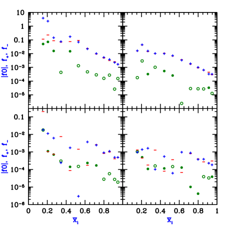
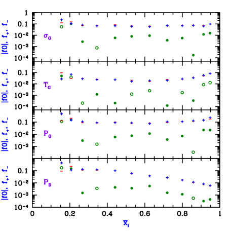
Specifically, we fit the four parameters $T_{G}$, $T_{L}$, $\sigma_{G}$, and $c_{G}$. We consider fitting the PDF in 5 $h^{-1}$Mpc boxes with MWA/10 or MWA/20 errors. Figure 12 shows that significant information can be reconstructed with MWA/10 errors, although the errors in the reconstructed parameters are usually fairly large (with particular failures at the early stage of reionization). The derived total probabilities of the GED model components are shown in Figure 13; in particular, the statistically significant measurement of the evolution of $P_{D}$ (which is the cosmic ionized fraction smoothed over the 5 $h^{-1}$Mpc resolution) shows that significant information can be extracted about the cosmic reionization history, even in this more flexible fitting approach.

Figure 12: Expected 1$\sigma$ errors on reconstructing the PDF parameters assuming the four-parameter GED model, assuming MWA/10 errors on the PDF in 5 $h^{-1}$Mpc boxes. We show the 16, 50, and 84 percentiles, as before, and also the assumed input values (circles).

Figure 13: Expected 1$\sigma$ errors on reconstructing the derived probabilities of the GED model, from a four-parameter fit to the PDF, assuming MWA/10 errors and 5 $h^{-1}$Mpc boxes. We show the 16, 50, and 84 percentiles, as before, and also the assumed input values (circles).

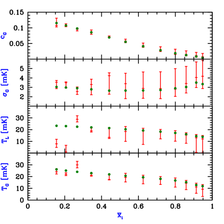
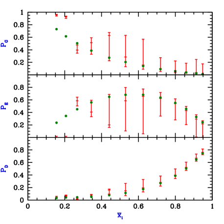
Since the errors on the reconstructed parameters with MWA/10 noise are still mostly of order unity, we explored further and found that MWA/20 is necessary to break most of the degeneracies. Figure 14 shows that in this case the parameters can usually be reconstructed to $1-10\%$ accuracy (with symmetric error bars and insignificant bias). Specifically we show the four quantities $P_{D}$, $P_{G}$, $T_{G}$ and $\sigma_{G}$, which together comprise a complete set that specifies the GED model. Note that the measurement of $P_{D}$ is particularly precise, during the latter stages of reionization.

Figure 14: Expected 1$\sigma$ errors on reconstructing various quantities of the GED model, from a four-parameter fit to the PDF, assuming MWA/20 errors and 5 $h^{-1}$Mpc boxes. As in the previous section, we show the relative errors $f_{0}$ (absolute value shown, where negative values are open circles and positive values are solid circles) , $f_{+}$ ($+$ symbols), and $f_{-}$ ($-$ symbols).

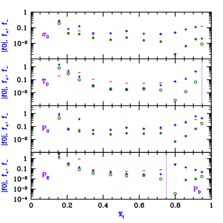
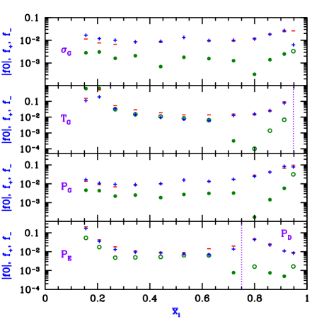
As in the previous section, the PDF in larger, 10 $h^{-1}$Mpc boxes, is easier to measure, due to the lower noise per pixel. Thus, here we consider somewhat larger noise levels, MWA/5 and MWA/10, with results shown in Figs. 15 and 16. Note that the last (highest $\bar{x}_{i}$) point in $T_{G}$ is not shown, since the input $T_{G}$ there is zero (see Figure 6), and also, we show $P_{D}$ only during late reionization, where it is non-zero (see Figure 7), and $P_{E}$ at earlier times. While the errors are fairly large with MWA/5 errors, they reach the $1-10\%$ level with MWA/10, corresponding to a second-generation 21-cm experiment.

Figure 15: Expected 1$\sigma$ errors on reconstructing various quantities of the GED model, from a four-parameter fit to the PDF, assuming MWA/5 errors and 10 $h^{-1}$Mpc boxes. We show the relative errors $f_{0}$ (absolute value shown, where negative values are open circles and positive values are solid circles) , $f_{+}$ ($+$ symbols), and $f_{-}$ ($-$ symbols).

Figure 16: Expected 1$\sigma$ errors on reconstructing various quantities of the GED model, from a four-parameter fit to the PDF, assuming MWA/10 errors and 10 $h^{-1}$Mpc boxes. We show the relative errors $f_{0}$ (absolute value shown, where negative values are open circles and positive values are solid circles) , $f_{+}$ ($+$ symbols), and $f_{-}$ ($-$ symbols).

6 Conclusions

We have carried out a detailed quantitative analysis of whether upcoming and future experiments can measure the shape of the 21-cm PDF and derive from it the cosmic reionization history. This is an important question since the PDF during reionization is highly non-Gaussian, it directly provides important information such as the cosmic ionization fraction at each redshift (though smoothed on the experimental resolution scale), and is potentially a way to derive the cosmic reionization history independently of the standard power spectrum analysis.

We developed a maximum-likelihood approach that achieves maximum efficiency by minimizing the $C$-statistic (eq. 6) applied to binned PDF data. We used a toy PDF model of two Gaussians (eq. 1) to show that the simplistic notion of signal-to-noise ratio (eq. 7) does not fully describe the ability to extract the PDF out of noisy data. Instead, once the noise per pixel rises above a few times the signal (i.e., the width of the intrinsic PDF), the errors blow up due to a strong degeneracy, even if the total signal-to-noise ratio is kept fixed by increasing the number of pixels (Figs. 1 and 2).

We measured the 21-cm PDF as a function of redshift in a large-scale N-body and radiative transfer simulation of cosmic reionization (Figs. 4 and 5). The PDF starts out close to Gaussian at high redshift, due to still-linear density fluctuations, later develops an exponential tail at low $T_{b}$, and finally becomes strongly peaked at zero towards the end of reionization. We empirically fit the PDF from the simulation with a four-parameter Gaussian + Exponential + Delta function (GED) model (eq. 10, Figs. 6 and 7).

Assuming the simulations as a reliable guide for the evolution of the PDF, we quantitatively explored how well parameters can be measured with two different approaches. In the most optimistic approach, we assumed that the real PDF matches the simulated one as a function of just a single free parameter, the ionization fraction $\bar{x}_{i}$, and tried to reconstruct this parameter from noisy mock data. We found that first-generation experiments (such as the MWA) are promising, at least if relatively large (10 $h^{-1}$Mpc) pixels are used along with their relatively low noise level per pixel. Specifically, a rather good measurement of the reionization history is expected in the mid to late stages of reionization, down to $1\%$ errors in measuring the cosmic mean ionized fraction.

We also considered reconstructing the cosmic reionization history together with the PDF shape, all while assuming that the four-parameter GED model correctly describes the real intrinsic PDF, but allowing the four parameters to vary freely when fitting mock data at each redshift. We found that this flexible approach requires much lower noise levels, characteristic of second-generation 21-cm experiments, to reach the level of $1-10\%$ accuracy in measuring the parameters of the 21-cm PDF.

We note that cosmic reionization ends in our simulation at redshift 7.5 (Fig. 3). If reionization in the real universe ends later (e.g., closer to $z=6.5$), then observations will be somewhat easier than we have assumed, due to the reduced foregrounds at lower redshift. On the simulation side, further work is necessary to establish the numerical convergence of the simulated 21-cm PDF during reionization, and to explore the dependence of the PDF on various astrophysical scenarios for the ionizing sources and sinks during reionization. This further effort is warranted since we have shown that the 21-cm PDF is a promising alternative to the power spectrum which can independently probe the cosmic reionization history.

References

- Barkana (2007) Barkana R., 2007, MNRAS, 376, 1784
- Barkana & Loeb (2001) Barkana, R., & Loeb, A. 2001, Phys. Rep., 349, 125
- Barkana & Loeb (2004) Barkana R., Loeb A., 2004, ApJ, 609, 474
- Barkana & Loeb (2007) Barkana R., Loeb A., 2007, Rep. Prog. Phys., 70, 627
- Barkana & Loeb (2008) Barkana, R., & Loeb, A. 2008, MNRAS, 384, 1069
- Bharadwaj & Ali (2005) Bharadwaj, S., & Pandey, S. K., 2005, MNRAS, 358, 968
- Bowman, Morales, & Hewitt (2006) Bowman J. D., Morales M. F., Hewitt J. N., 2006, ApJ, 638, 20
- Cash (1979) Cash W., 1979, ApJ, 228, 939
- Ciardi & Madau (2003) Ciardi B., Madau, P., 2003, ApJ, 596, 1
- Furlanetto et al. (2004) Furlanetto S. R., Zaldarriaga M., Hernquist L., 2004, ApJ, 613, 1
- Furlanetto et al. (2006) Furlanetto S. R., Oh S. P., Briggs, F., 2006, Phys. Rep., 433, 181
- Harker et al. (2009) Harker, G. J. A., et al. 2009, MNRAS, 393, 1449
- Iliev et al. (2006a) Iliev I. T., et al., 2006a, MNRAS, 371, 1057
- Iliev et al. (2006b) Iliev I. T., Mellema G., Pen U.-L., Merz H., Shapiro P. R., Alvarez M. A., 2006b, MNRAS, 369, 1625
- Iliev et al. (2007) Iliev I. T., Mellema G., Shapiro P. R., Pen U.-L. 2007, MNRAS, 376, 534
- Iliev et al. (2008) Iliev I. T., Mellema G., Pen U.-L., Bond J. R., Shapiro P. R. 2008, MNRAS, 384, 863
- Iliev et al. (2009) Iliev I. T., et al., 2009, arXiv0905.2920
- Madau et al. (1997) Madau, P., Meiksin, A., & Rees, M. J. 1997, ApJ, 475, 429
- McQuinn et al. (2005) McQuinn M., Furlanetto S. R., Hernquist L., Zahn O., Zaldarriaga M., 2005, ApJ, 630, 643
- McQuinn et al. (2006) McQuinn M., Zahn O., Zaldarriaga M., Hernquist L., Furlanetto S. R., 2006, ApJ, 653, 815
- Mellema et al. (2006a) Mellema G., Iliev I. T., Alvarez M. A., Shapiro P. R., 2006a, New Astronomy, 11, 374
- Mellema et al. (2006b) Mellema G., Iliev I. T., Pen U.-L., Shapiro P. R., 2006b, MNRAS, 372, 679
- Merz et al. (2005) Merz H., Pen U.-L., Trac H., 2005, New Astronomy, 10, 393
- Oh et al. (2009) Oh S. P., Hansen M., Furlanetto S. R., Mesinger A., 2009, submitted
- Saiyad-Ali et al. (2006) Saiyad-Ali, S., Bharadwaj, S., & Pandey, S. K., 2006, MNRAS, 366, 213
- Santos et al. (2008) Santos M. G., Amblard A., Pritchard J., Trac H., Cen R., Cooray A. 2008, ApJ, 689, 1
- Spergel et al. (2007) Spergel, D. N., et al., 2007, ApJS, 170, 377
- Wyithe & Morales (2007) Wyithe S., Morales M., 2007, MNRAS, 379, 1647
- Zahn et al. (2007) Zahn O., Lidz A., McQuinn M., Dutta S., Hernquist L., Zaldarriaga M., Furlanetto S. R., 2007, ApJ, 654, 12