Numerical calculation of second order perturbations

Abstract

We numerically solve the Klein-Gordon equation at second order in cosmological perturbation theory in closed form for a single scalar field, describing the method employed in detail. We use the slow-roll version of the second order source term and argue that our method is extendable to the full equation. We consider two standard single field models and find that the results agree with previous calculations using analytic methods, where comparison is possible. Our procedure allows the evolution of second order perturbations in general and the calculation of the non-linearity parameter $f_{\mathrm{NL}}$ to be examined in cases where there is no analytical solution available.

I Introduction

Cosmological perturbation theory is an essential tool for the analysis of cosmological models, in particular as the amount of observational data continues to increase. With the recent launch of the planck satellite, the wmap mission reaching its eighth year, and a host of other new experiments, we will have access to more information about the early universe than ever before planck ; Komatsu:2008hk .

To distinguish between theoretical models it is necessary to go beyond the standard statistical analyses that have been so successful in the recent past. As a result much interest has been focused on non-gaussianity as a new tool to help classify and test models of the early universe. Perturbation theory beyond first order will be required to make the best possible use of the data. In this paper we outline an important step in the understanding of perturbation theory beyond first order, demonstrating that second order perturbations are readily amenable to numerical calculation, even on small and intermediate scales inside the horizon.

Inflationary model building has for the past few years focused on meeting the requirements of first order perturbation theory, namely that the power spectra of scalar and tensor perturbations should match that observed in the Cosmic Microwave Background (CMB). Inflationary models are classified and tested based on their predictions for the power spectrum of curvature perturbations, the spectral index of these perturbations and the ratio of tensor to scalar perturbations. As the potential for moving beyond first order perturbations has been explored, these three observable quantities have been joined by a measure of the departure from gaussianity exhibited by the perturbations, the non-gaussianity parameter $f_{\mathrm{NL}}$. This parameter is not yet well constrained by observational data in comparison with the other quantities but can already be used to rule out models with particularly strong non-gaussian signatures.

There are two main approaches to studying higher order effects and non-gaussianity. One approach uses nonlinear theory and a gradient expansion in various guises, either explicitly, e.g. Refs. Salopek:1990jq ; Rigopoulos:2005xx or in the form of the $\Delta N$ formalism, e.g. Refs. Starobinsky:1982ee ; Starobinsky:1986fxa ; Sasaki:1995aw ; Sasaki:1998ug ; Lyth:2004gb ; Lyth:2005fi ; Langlois:2006vv By virtue of having to employ a gradient expansion this approach is so far only usable on scales much larger than the particle horizon. The other approach uses cosmological perturbation theory following Bardeen Bardeen:1980kt and extending it to second order, e.g. Refs. Tomita:1967 ; Mukhanov:1996ak ; Bruni:1996im ; Acquaviva:2002ud ; Nakamura:2003wk ; Noh:2004bc ; Bernardeau:2002jy ; Maldacena:2002vr ; Finelli:2003bp ; Bartolo:2004if ; Enqvist:2004bk ; Lyth:2005du ; Seery:2005gb ; Malik:2003mv ; Barnaby:2006cq (for an extensive list of references and a recent review on these issues see Ref. Malik:2008im ). This approach works on all scales, but can be more complex than in particular the $\Delta N$ formalism. Both these approaches give the same results on large scales Malik:2005cy . We will follow the Bardeen approach in this paper.

As the first order perturbations of the inflaton field are taken in the standard treatment to be purely gaussian it is in general necessary to go to second order in order to understand and estimate the non-gaussian contribution of any inflationary model (for a recent review see Ref. Malik:2008im ). Deriving the equations of motion is not trivial at second order and only recently was the Klein-Gordon equation for scalar fields derived in closed form, taking into account metric backreaction Malik:2006ir . This allows for the first time a direct computation of the second order perturbation in full, in contrast with previous attempts which have focused only on certain terms in the expression, for example Ref. Finelli:2006wk .

In this paper we solve numerically the second order Klein-Gordon equation in closed form in Fourier space and show that this procedure is readily applicable to the study of non-gaussianity and other higher order effects. As this is, to our knowledge, the first numerical solution to the full second order evolution equation we will outline the numerical steps taken in the system we have developed, examine the current constraints on the calculation and describe the next steps required in detail. This calculation uses the slow roll version of the second order equation, but solves the full non-slow roll equations for the background and first order. The models that we test in this paper are single field models with a canonical action. Significant second order corrections are expected only when a non-canonical action or multiple fields are used, or slow roll is violated. Numerical simulations will be particularly useful in analysing models with these characteristics. We will discuss in Section V planned future work to extend our current numerical system to deal with these extensions beyond the standard single field slow roll inflation.

In Section II we will give a brief outline of perturbation theory and describe the second order perturbation equations that will be numerically calculated. Section III describes the numerical implementation of the calculation, including the initial conditions used and the computational requirements. We present the results of this calculation in Section IV including a comparison of the second order perturbation calculated for the $\frac{1}{2}m^{2}\varphi^{2}$ and $\frac{1}{4}\lambda\varphi^{4}$ potentials. We will discuss these results and the next stages of this work in Section V.

Throughout this paper we set $\hbar=c=1$ and use the reduced Planck mass $M_{\mathrm{PL}}=\sqrt{8\pi G}$. Overdots and primes denote differentiation with respect to our time variable $n$ (the number of e-foldings) and conformal time $\eta$, respectively, and will be defined explicitly when first used. We will work in a flat Friedmann-Robertson-Walker (FRW) background.

II Perturbations

In this section we will briefly review the derivation of first and second order perturbations in the uniform curvature gauge and describe the slow roll approximation that we will use in this paper. There are many reviews on the subject of cosmological perturbation theory, and here we will follow Ref. Malik:2008im . The full closed Klein-Gordon equation for second order perturbations was recently given by one of the authors and we will outline the derivation in Ref. Malik:2006ir below.

II.1 First and Second Order

In this paper we will consider perturbations of a single scalar field and will work throughout in the uniform curvature or flat gauge. Our goal is to describe scalar perturbations up to second order and the first step to achieve this is to examine the metric tensor:

$$g_{00} = -a^{2}\left(1+2\phi_{1}+\phi_{2}\right)\,,$$ (1)

$$g_{0i} = a^{2}\left(B_{1}+\frac{1}{2}B_{2}\right)_{,i}\,,$$ (2)

$$g_{ij} = a^{2}\left[\left(1-2\psi_{1}-\psi_{2}\right)\delta_{ij}+2E_{1,ij}+E_{2,ij}\right]\,,$$ (3)

where $a=a(\eta)$ is the scale factor, $\eta$ conformal time, $\delta_{ij}$ is the flat background metric, $\phi_{1}$ and $\phi_{2}$ the lapse functions, and $\psi_{1}$ and $\psi_{2}$ the curvature perturbations at first and second order; $B_{1}$ and $B_{2}$ and $E_{1}$ and $E_{2}$ are scalar perturbations describing the shear. Spatial 3-hypersurfaces are flat in our chosen gauge and so

$$\widetilde{\psi}_{1}=\widetilde{\psi}_{2}=\widetilde{E}_{1}=\widetilde{E}_{2}=0\,,$$ (4)

where the tilde denotes quantities in flat gauge.

The Sasaki-Mukhanov variable, i.e. the field perturbation on uniform curvature hypersurfaces Sasaki:1986hm ; Mukhanov:1988jd , evaluated at first order is given by

$$\widetilde{{\delta\varphi_{1}}}={\delta\varphi_{1}}+\frac{{\varphi}_{0}^{\prime}}{\mathcal{H}}\psi_{1}\,,$$ (5)

where ${\varphi}_{0}$ is the background value of the field and the perturbations of $\varphi$ are defined as

$$\varphi(x^{\mu})={\varphi}_{0}(\eta)+{\delta\varphi_{1}}(\eta,x^{i})+\frac{1}{2}{\delta\varphi_{2}}(\eta,x^{i})\,.$$ (6)

At second order the Sasaki-Mukhanov variable becomes more complicated Malik:2005cy ; Malik:2003mv :

$$\widetilde{{\delta\varphi_{2}}}={\delta\varphi_{2}}+\frac{{\varphi}_{0}^{\prime}}{\mathcal{H}}\psi_{2}+\left(\frac{\psi_{1}}{\mathcal{H}}\right)^{2}\left[2\mathcal{H}{\varphi}_{0}^{\prime}+{\varphi}_{0}^{\prime\prime}-\frac{\mathcal{H}^{\prime}}{\mathcal{H}}{\varphi}_{0}^{\prime}\right]+2\frac{{\varphi}_{0}^{\prime}}{\mathcal{H}^{2}}\psi_{1}^{\prime}\psi_{1}+\frac{2}{\mathcal{H}}\psi_{1}{\delta\varphi_{1}}^{\prime}-2\delta{\varphi}_{1,k}E_{1,}^{~{}k}+{\cal{X}}\left(\psi,E\right)\,,$$ (7)

where ${\cal{X}}\left(\psi,E\right)$ contains terms quadratic in gradients of the metric perturbations $\psi_{1}$ and $E_{1}$. From now on we will drop the tildes and talk only about variables in the flat gauge. The potential of the scalar field is also split

$$U(\varphi)=U_{0}+\delta U_{1}+\frac{1}{2}\delta U_{2}\,,\quad\delta U_{1}=U_{,\varphi}{\delta\varphi_{1}}\,,\quad\delta U_{2}=U_{,\varphi\varphi}{\delta\varphi_{1}}^{2}+U_{,\varphi}{\delta\varphi_{2}}\,,$$ (8)

where $U_{,\varphi}=\frac{\partial U}{\partial\varphi}$. The Klein-Gordon equation describes the evolution of the scalar field. For the background field we have

$${\varphi}_{0}^{\prime\prime}+2\mathcal{H}{\varphi}_{0}^{\prime}+a^{2}U_{,\varphi}=0\,,$$ (9)

where $\mathcal{H}\equiv\frac{a^{\prime}}{a}$ is related to the Hubble parameter $H$ by $\mathcal{H}=aH$. The first order equation is

$${\delta\varphi_{1}}^{\prime\prime}+2\mathcal{H}{\delta\varphi_{1}}^{\prime}+2a^{2}U_{,\varphi}\phi_{1}-\nabla^{2}{\delta\varphi_{1}}-{\varphi}_{0}^{\prime}\nabla^{2}B_{1}-{\varphi}_{0}^{\prime}\phi^{\prime}_{1}+a^{2}U_{,\varphi\varphi}{\delta\varphi_{1}}=0\,,$$ (10)

and the second order

$${\delta\varphi_{2}}^{\prime\prime} + 2\mathcal{H}{\delta\varphi_{2}}^{\prime}-\nabla^{2}{\delta\varphi_{2}}+a^{2}U_{,\varphi\varphi}{\delta\varphi_{2}}+a^{2}U_{,\varphi\varphi\varphi}({\delta\varphi_{1}})^{2}+2a^{2}U_{,\varphi}\phi_{2}-{\varphi}_{0}^{\prime}\left(\nabla^{2}B_{2}+\phi_{2}^{\prime}\right)$$ (11)

$$+ 4{\varphi}_{0}^{\prime}B_{1,k}\phi_{1,}^{~{}k}+2\left(2\mathcal{H}{\varphi}_{0}^{\prime}+a^{2}U_{,\varphi}\right)B_{1,k}B_{1,}^{~{}k}+4\phi_{1}\left(a^{2}U_{,\varphi\varphi}{\delta\varphi_{1}}-\nabla^{2}{\delta\varphi_{1}}\right)+4{\varphi}_{0}^{\prime}\phi_{1}\phi_{1}^{\prime}$$

$$- 2{\delta\varphi_{1}}^{\prime}\left(\nabla^{2}B_{1}+\phi_{1}^{\prime}\right)-4{\delta\varphi_{1}}^{\prime}_{,k}B_{1,}^{~{}k}=0\,,$$

where as mentioned before all the variables are now in the flat gauge.

The Einstein field equations are also required at first and second order. We will not reproduce them here but instead refer the interested reader to Section II B of Ref. Malik:2006ir . Using the perturbed Einstein equations, the Klein-Gordon equations above can be written in closed form at both first and second orders. These equations will form the basis of the numerical scheme described in Section III.

The dynamics of the scalar field becomes clearer in Fourier space but terms in the second order equation of the form $\left({\delta\varphi_{1}}(x)\right)^{2}$ require the use of the convolution theorem (see for example Ref. Vretblad:2005 ). Following Refs. Malik:2006ir and book:liddle we will write ${\delta\varphi}(k^{i})$ for the Fourier component of ${\delta\varphi}(x)$ such that

$${\delta\varphi}(\eta,x^{i})=\frac{1}{(2\pi)^{3}}\int d^{3}k{\delta\varphi}({{k^{i}}})\exp(ik_{i}x^{i})\,,$$ (12)

where ${{k^{i}}}$ is the comoving wavenumber.

In Fourier space the closed form of the first order Klein-Gordon equation transforms into

$${\delta\varphi_{1}}({{k^{i}}})^{\prime\prime}+2\mathcal{H}{\delta\varphi_{1}}({{k^{i}}})^{\prime}+k^{2}{\delta\varphi_{1}}({{k^{i}}})+a^{2}\left[U_{,\varphi\varphi}+\frac{8\pi G}{\mathcal{H}}\left(2{\varphi}_{0}^{\prime}U_{,\varphi}+({\varphi}_{0}^{\prime})^{2}\frac{8\pi G}{\mathcal{H}}U_{0}\right)\right]{\delta\varphi_{1}}({{k^{i}}})=0\,.$$ (13)

As mentioned above the second order equation requires more careful consideration with terms quadratic in the first order perturbation, which require convolutions of the form

$$f(x)g(x)\longrightarrow\frac{1}{(2\pi)^{3}}\int d^{3}qd^{3}p\,\delta^{3}({{k^{i}}}-{{p^{i}}}-{{q^{i}}})f({{p^{i}}})g(q^{i})\,.$$ (14)

For convenience we will group the terms with gradients of ${\delta\varphi_{1}}(x)$ together and denote them by $F$. The full closed form second order Klein-Gordon equation in Fourier Space is

$${\delta\varphi_{2}}^{\prime\prime}({{k^{i}}})+2\mathcal{H}{\delta\varphi_{2}}^{\prime}({{k^{i}}})+k^{2}{\delta\varphi_{2}}({{k^{i}}})+a^{2}\left[U_{,\varphi\varphi}+\frac{8\pi G}{\mathcal{H}}\left(2{\varphi}_{0}^{\prime}U_{,\varphi}+({\varphi}_{0}^{\prime})^{2}\frac{8\pi G}{\mathcal{H}}U_{0}\right)\right]{\delta\varphi_{2}}({{k^{i}}})$$

$$+\frac{1}{(2\pi)^{3}}\int d^{3}qd^{3}p\,\delta^{3}({{k^{i}}}-{{p^{i}}}-{{q^{i}}})\left\{\frac{16\pi G}{\mathcal{H}}\left[X{\delta\varphi_{1}}^{\prime}({{p^{i}}}){\delta\varphi_{1}}({{q^{i}}})+{\varphi}_{0}^{\prime}a^{2}U_{,\varphi\varphi}{\delta\varphi_{1}}({{p^{i}}}){\delta\varphi_{1}}({{q^{i}}})\right]\right.$$

$$+\left(\frac{8\pi G}{\mathcal{H}}\right)^{2}{\varphi}_{0}^{\prime}\left[2a^{2}U_{,\varphi}{\varphi}_{0}^{\prime}{\delta\varphi_{1}}({{p^{i}}}){\delta\varphi_{1}}({{q^{i}}})+{\varphi}_{0}^{\prime}X{\delta\varphi_{1}}({{p^{i}}}){\delta\varphi_{1}}({{q^{i}}})\right]$$

$$-2\left(\frac{4\pi G}{\mathcal{H}}\right)^{2}\frac{{\varphi}_{0}^{\prime}X}{\mathcal{H}}\left[X{\delta\varphi_{1}}({{p^{i}}}){\delta\varphi_{1}}({{q^{i}}})+{\varphi}_{0}^{\prime}{\delta\varphi_{1}}({{p^{i}}}){\delta\varphi_{1}}^{\prime}({{q^{i}}})\right]$$

$$\left.+\frac{4\pi G}{\mathcal{H}}{\varphi}_{0}^{\prime}{\delta\varphi_{1}}^{\prime}({{p^{i}}}){\delta\varphi_{1}}^{\prime}({{q^{i}}})+a^{2}\left[U_{,\varphi\varphi\varphi}+\frac{8\pi G}{\mathcal{H}}{\varphi}_{0}^{\prime}U_{,\varphi\varphi}\right]{\delta\varphi_{1}}({{p^{i}}}){\delta\varphi_{1}}({{q^{i}}})\right\}$$

$$+F({\delta\varphi_{1}}({{k^{i}}}),{\delta\varphi_{1}}^{\prime}({{k^{i}}}))=0\,.$$ (15)

Here we use $X=a^{2}(8\pi GU_{0}{\varphi}_{0}^{\prime}/\mathcal{H}+U_{,\varphi})$ for convenience. The $F$ term contains gradients of ${\delta\varphi_{1}}$ in real space and therefore the convolution integrals include additional factors of $k$ and $q$. It is given by

$$F\left({\delta\varphi_{1}}({{k^{i}}}),{\delta\varphi_{1}}^{\prime}({{k^{i}}})\right)=\frac{1}{(2\pi)^{3}}\int d^{3}pd^{3}q\delta^{3}({{k^{i}}}-{{p^{i}}}-{{q^{i}}})\Bigg{\{}2\left(\frac{8\pi G}{\mathcal{H}}\right)\frac{p_{k}q^{k}}{q^{2}}\delta{\varphi}_{1}^{\prime}({{p^{i}}})\left(X{\delta\varphi_{1}}({{q^{i}}})+{\varphi}_{0}^{\prime}{\delta\varphi_{1}}^{\prime}({{q^{i}}})\right)$$

$$+p^{2}\frac{16\pi G}{\mathcal{H}}{\delta\varphi_{1}}({{p^{i}}}){\varphi}_{0}^{\prime}{\delta\varphi_{1}}({{q^{i}}})+\left(\frac{4\pi G}{\mathcal{H}}\right)^{2}\frac{{\varphi}_{0}^{\prime}}{\mathcal{H}}\Bigg{[}\left(p_{l}q^{l}-\frac{p^{i}q_{j}k^{j}k_{i}}{k^{2}}\right){\varphi}_{0}^{\prime}\delta{\varphi}_{1}({{p^{i}}}){\varphi}_{0}^{\prime}\delta{\varphi}_{1}({{q^{i}}})\Bigg{]}$$

$$+2\frac{X}{\mathcal{H}}\left(\frac{4\pi G}{\mathcal{H}}\right)^{2}\frac{p_{l}q^{l}p_{m}q^{m}+p^{2}q^{2}}{k^{2}q^{2}}\Bigg{[}{\varphi}_{0}^{\prime}\delta{\varphi}_{1}({{p^{i}}})\left(X{\delta\varphi_{1}}({{q^{i}}})+{\varphi}_{0}^{\prime}{\delta\varphi_{1}}^{\prime}({{q^{i}}})\right)\Bigg{]}$$

$$+\frac{4\pi G}{\mathcal{H}}\Bigg{[}4X\frac{q^{2}+p_{l}q^{l}}{k^{2}}\left({\delta\varphi_{1}}^{\prime}({{p^{i}}}){\delta\varphi_{1}}({{q^{i}}})\right)-{\varphi}_{0}^{\prime}p_{l}q^{l}\delta{\varphi}_{1}({{p^{i}}})\delta{\varphi}_{1}({{q^{i}}})\Bigg{]}$$

$$+\left(\frac{4\pi G}{\mathcal{H}}\right)^{2}\frac{{\varphi}_{0}^{\prime}}{\mathcal{H}}\Bigg{[}\frac{p_{l}q^{l}p_{m}q^{m}}{p^{2}q^{2}}\left(X{\delta\varphi_{1}}({{p^{i}}})+{\varphi}_{0}^{\prime}{\delta\varphi_{1}}^{\prime}({{p^{i}}})\right)\left(X{\delta\varphi_{1}}({{q^{i}}})+{\varphi}_{0}^{\prime}{\delta\varphi_{1}}^{\prime}({{q^{i}}})\right)\Bigg{]}$$

$$+\frac{{\varphi}_{0}^{\prime}}{\mathcal{H}}\Bigg{[}8\pi G\left(\frac{p_{l}q^{l}+p^{2}}{k^{2}}q^{2}{\delta\varphi_{1}}({{p^{i}}}){\delta\varphi_{1}}({{q^{i}}})-\frac{q^{2}+p_{l}q^{l}}{k^{2}}{\delta\varphi_{1}}^{\prime}({{p^{i}}}){\delta\varphi_{1}}^{\prime}({{q^{i}}})\right)$$

$$\qquad\qquad\qquad+\left(\frac{4\pi G}{\mathcal{H}}\right)^{2}\frac{k^{j}k_{i}}{k^{2}}\Bigg{(}2\frac{p^{i}p_{j}}{p^{2}}\left(X{\delta\varphi_{1}}({{p^{i}}})+{\varphi}_{0}^{\prime}{\delta\varphi_{1}}^{\prime}({{p^{i}}})\right)X{\delta\varphi_{1}}({{q^{i}}})\Bigg{)}\Bigg{]}\Bigg{\}}\,.$$ (16)

II.2 Slow Roll approximation

In order to establish the viability of a numerical calculation of the Klein-Gordon equation we have confined ourselves in this paper to studying the evolution in the slow roll approximation. In our case this involves taking

$${\varphi}_{0}^{\prime\prime}=\mathcal{H}{\varphi}_{0}^{\prime}\simeq 0\,,\quad\frac{\left({\varphi}_{0}^{\prime}\right)^{2}}{2a^{2}}\ll U_{0}\,,$$ (17)

such that $X=0$ and $\mathcal{H}^{2}=(8\pi G/3)a^{2}U_{0}$. The slow roll parameter $\epsilon_{H}$ as defined in Refs. Malik:2006ir and Seery:2005gb (which is the square-root of the usual $\epsilon$) is given by

$$\varepsilon_{H}=\sqrt{4\pi G}\frac{{\varphi}_{0}^{\prime}}{\mathcal{H}}\,.$$ (18)

With this approximation the second order equation (II.1) simplifies dramatically, and with the $F$ term included is

$${\delta\varphi_{2}}^{\prime\prime}({{k^{i}}})+2\mathcal{H}{\delta\varphi_{2}}^{\prime}({{k^{i}}})+k^{2}{\delta\varphi_{2}}({{k^{i}}})+\left(a^{2}U_{,\varphi\varphi}-{24\pi G}({\varphi}_{0}^{\prime})^{2}\right){\delta\varphi_{2}}({{k^{i}}})$$ (19)

$$+\int d^{3}p\ d^{3}q\ \delta^{3}({{k^{i}}}-{{p^{i}}}-{{q^{i}}})\Bigg{\{}a^{2}\left(U_{,\varphi\varphi\varphi}+\frac{8\pi G}{\mathcal{H}}{\varphi}_{0}^{\prime}U_{,\varphi\varphi}\right){\delta\varphi_{1}}({{p^{i}}}){\delta\varphi_{1}}({{q^{i}}})+\frac{16\pi G}{\mathcal{H}}a^{2}{\varphi}_{0}^{\prime}U_{,\varphi\varphi}{\delta\varphi_{1}}({{p^{i}}}){\delta\varphi_{1}}({{q^{i}}})\Bigg{\}}$$

$$+\frac{8\pi G}{\mathcal{H}}\int d^{3}p\ d^{3}q\ \delta^{3}({{k^{i}}}-{{p^{i}}}-{{q^{i}}})\Bigg{\{}\frac{8\pi G}{\mathcal{H}}\frac{p_{l}q^{l}}{q^{2}}{\varphi}_{0}^{\prime}{\delta\varphi_{1}}^{\prime}({{p^{i}}}){\delta\varphi_{1}}^{\prime}({{q^{i}}})+2p^{2}{\varphi}_{0}^{\prime}{\delta\varphi_{1}}({{p^{i}}}){\delta\varphi_{1}}({{q^{i}}})$$

$$\qquad\qquad\qquad\qquad+{\varphi}_{0}^{\prime}\Bigg{(}\left(\frac{p_{l}q^{l}+p^{2}}{k^{2}}q^{2}-\frac{p_{l}q^{l}}{2}\right){\delta\varphi_{1}}({{p^{i}}}){\delta\varphi_{1}}({{q^{i}}})+\left(\frac{1}{2}-\frac{q^{2}+p_{l}q^{l}}{k^{2}}\right){\delta\varphi_{1}}^{\prime}({{p^{i}}}){\delta\varphi_{1}}^{\prime}({{q^{i}}})\Bigg{)}\Bigg{\}}=0\,.$$

The numerical simulation in this paper will solve the slow roll version of the second order above, Eq. (19), the first order equation (13) and the background equation (9). In the next section we set up the correct form of these equations for the numerical simulation and discuss the implementation and some tests of the accuracy of the method.

III Numerics

Our goal in this paper is to show that, just as at first order, a direct numerical calculation of the second order perturbations of a scalar field system is achievable and in this section we will outline how we have implemented this system. In structuring the numerical system we have closely followed the work done at first order by Martin and Ringeval Martin:2006rs ; Ringeval:2007am and previously by Salopek et al. Salopek:1988qh .

A finite numerical range of $k$ modes to be calculated is required. The upper cutoff in $k$, which marks the smallest scale considered, is well motivated by the difficulty in observing primordial perturbations at these small scales. At the other end we need to specify the largest scale or smallest $k$ that we will consider. Analytically this is often taken to be the size of the universe, with $k=0$ being the equivalent mode. One immediate problem with this is that the Bunch-Davies vacuum initial conditions outlined in Section III.2 blow up. The standard workaround is to implement a cutoff at large scales beyond which the amplitude of perturbations is zero. This is a pragmatic approach but recently there has been some evidence that a sharp cutoff similar to this could be responsible for the lack of power at large scales in the WMAP data Lyth:2007jh ; spergel ; Sinha:2005mn ; Kim:2009pf .

The main concern is that the $k$ range covers most if not all the modes observed to date in the CMB. The WMAP team rely for their main results, Komatsu:2008hk , on $\ell$ multipoles in the range $\ell\in[3,1000]$ which corresponds approximatelyto $k\in\left[0.92{\times 10^{-60}},3.1\times 10^{-58}\right]M_{\mathrm{PL}}=\left[3.5{\times 10^{-4}},0.12\right]M\mathrm{pc}^{-1}$. We will consider a similar range of $k$ modes in this paper, taking three different ranges outlined in Section IV. The choice of $k$ range is flexible with the only constraint being that the number of modes at second order is one greater than a power of two. This enables faster integration using the Romberg method as explained below.

III.1 Equations

The equations in Section II.2 are not set up for a numerical calculation and in this section we rearrange them into a more suitable form. This involves a change of time coordinate and grouping of terms into smaller units for calculation. The second order slow roll equation (19) can be further simplified by performing the $p$ integral and changing to spherical polar coordinates $q,\theta,\omega$ where $q=|\textbf{q}|$. The $d^{3}q$ integral becomes

$$\int d^{3}q\longrightarrow\int_{0}^{\infty}q^{2}dq\int_{0}^{\pi}\sin\theta d\theta\int_{0}^{2\pi}d\omega\,.$$ (20)

For each $k$ mode equation we take the $\theta=0,\omega=0$ axis in the direction of ${{k^{i}}}$, so that the angle between ${{k^{i}}}$ and ${{q^{i}}}$ is $\theta$ and the scalar product $q_{i}k^{i}=qk\cos\theta$. The argument of each ${\delta\varphi_{1}}$ or ${\delta\varphi_{1}}^{\prime}$ term depends on $\theta$ through $|{{k^{i}}}-{{q^{i}}}|=\sqrt{k^{2}+q^{2}-2kq\cos\theta}$ and so must remain inside the $\theta$ integral. There is no $\omega$ dependence in ${\delta\varphi_{1}}$ with this choice of axes, so the last integral is simply evaluated.

In the slow roll case there are only four different $\theta$ dependent terms, here labelled A–D:

$$A({{k^{i}}},{{q^{i}}}) = \int_{0}^{\pi}\sin(\theta){\delta\varphi_{1}}({{k^{i}}}-{{q^{i}}})d\theta\,,$$

$$B({{k^{i}}},{{q^{i}}}) = \int_{0}^{\pi}\cos(\theta)\sin(\theta){\delta\varphi_{1}}({{k^{i}}}-{{q^{i}}})d\theta\,,$$

$$C({{k^{i}}},{{q^{i}}}) = \int_{0}^{\pi}\sin(\theta){\delta\varphi_{1}}^{\prime}({{k^{i}}}-{{q^{i}}})d\theta\,,$$

$$D({{k^{i}}},{{q^{i}}}) = \int_{0}^{\pi}\cos(\theta)\sin(\theta){\delta\varphi_{1}}^{\prime}({{k^{i}}}-{{q^{i}}})d\theta\,.$$ (21)

Written using the terms in Eqs. (III.1) the slow roll equation (19) becomes:

$${\delta\varphi_{2}}^{\prime\prime}({{k^{i}}})+2\mathcal{H}{\delta\varphi_{2}}^{\prime}({{k^{i}}})+k^{2}{\delta\varphi_{2}}({{k^{i}}})+\left(a^{2}U_{,\varphi\varphi}-{24\pi G}({\varphi}_{0}^{\prime})^{2}\right){\delta\varphi_{2}}({{k^{i}}})+S({{k^{i}}})=0\,,$$ (22)

$$S({{k^{i}}})=\frac{1}{(2\pi)^{2}}\int dq\ \Bigg{\{}a^{2}U_{,\varphi\varphi\varphi}q^{2}{\delta\varphi_{1}}({{q^{i}}})A({{k^{i}}},{{q^{i}}})$$ (23)

$$\qquad\qquad\qquad\qquad\qquad+\frac{8\pi G}{\mathcal{H}}{\varphi}_{0}^{\prime}\Bigg{[}\left(3a^{2}U_{,\varphi\varphi}+\frac{7}{2}q^{4}+2k^{2}q^{2}\right)A({{k^{i}}},{{q^{i}}})-\left(\frac{9}{2}+\frac{q^{2}}{k^{2}}\right)kq^{3}B({{k^{i}}},{{q^{i}}})\Bigg{]}{\delta\varphi_{1}}({{q^{i}}})$$

$$\qquad\qquad\qquad\qquad\qquad+\frac{8\pi G}{\mathcal{H}}{\varphi}_{0}^{\prime}\Bigg{[}-\frac{3}{2}q^{2}C({{k^{i}}},{{q^{i}}})+\left(2-\frac{q^{2}}{k^{2}}\right)kqD({{k^{i}}},{{q^{i}}})\Bigg{]}{\delta\varphi_{1}}^{\prime}({{q^{i}}})\Bigg{\}}\,,$$

where $S({{k^{i}}})$ is the source term which will be determined before the second order system is run. The full set of equations which must be evolved are then Eq. (9) for the background, Eq. (13) for the first order perturbations and Eqs. (22) and (23) for the second order and source terms.

A more appropriate time variable for the numerical simulation is the number of e-foldings, and hence we use

$$n=\log(a/a_{\mathrm{init}})\,,$$ (24)

as our time variable instead of conformal time. Here, $a_{\mathrm{init}}$ is the value of $a$ at the beginning of the simulation. If $a$ is set to be $1$ today we can calculate $a_{\mathrm{init}}$ once the background run is complete and the end time of inflation is determined as in Section III.3. We will use an overdot to denote differentiation with respect to $n$.

The changes in derivatives required are as follows:

$$\frac{\partial}{\partial\eta} = \frac{dn}{d\eta}\frac{\partial}{\partial n}=\mathcal{H}\frac{\partial}{\partial n}\,,$$ (25)

$$\frac{\partial}{\partial t} = \frac{d\eta}{dt}\frac{dn}{d\eta}\frac{\partial}{\partial n}=H\frac{\partial}{\partial n}\,,$$ (26)

where $\eta$ and $t$ are conformal and coordinate time respectively with $H=\frac{da}{dt}/a$ and $\mathcal{H}=aH$. As mentioned above the value of $a$ at the end of inflation is calculated using the connection equation (see for example Eq. (3.19) in Ref. book:liddle or Eq. (7) in Ref. Peiris:2008be ) assuming that instantaneous reheating occurs at the end of inflation. This gives approximately 65 e-foldings from the end of inflation until now. The background and first order equations written in terms of the new time variable $n$ are

$$\ddot{{\varphi}_{0}}+\frac{U_{0}}{H^{2}}\dot{{\varphi}_{0}}+\frac{U_{,\varphi}}{H^{2}}=0\,,$$ (27)

$$\ddot{{\delta\varphi_{1}}}+\left(3+\frac{\dot{H}}{H}\right)\dot{{\delta\varphi_{1}}}+\left[\left(\frac{k}{aH}\right)^{2}+\frac{U_{,\varphi\varphi}}{H^{2}}+\frac{8\pi G}{H^{2}}2\dot{{\varphi}_{0}}U_{,\varphi}+\left(\frac{8\pi G}{H}\right)^{2}\left(\dot{{\varphi}_{0}}\right)^{2}U_{0}\right]{\delta\varphi_{1}}=0\,.$$ (28)

The second order equation in terms of $n$ is

$$\ddot{{\delta\varphi_{2}}}({{k^{i}}})+\left(3+\frac{\dot{H}}{H}\right)\dot{{\delta\varphi_{2}}}({{k^{i}}})+\left(\frac{k}{aH}\right)^{2}{\delta\varphi_{2}}({{k^{i}}})+\left(\frac{U_{,\varphi\varphi}}{H^{2}}-{24\pi G}(\dot{{\varphi}_{0}})^{2}\right){\delta\varphi_{2}}({{k^{i}}})+S({{k^{i}}})=0\,,$$ (29)

$$S({{k^{i}}}) = \frac{1}{(2\pi)^{2}}\int dq\ \Bigg{\{}\frac{U_{,\varphi\varphi\varphi}}{H^{2}}q^{2}{\delta\varphi_{1}}({{q^{i}}})A({{k^{i}}},{{q^{i}}})$$ (30)

$$+\,\frac{8\pi G}{(aH)^{2}}\dot{{\varphi}_{0}}\Bigg{[}\left(3a^{2}U_{,\varphi\varphi}q^{2}+\frac{7}{2}q^{4}+2k^{2}q^{2}\right)A({{k^{i}}},{{q^{i}}})-\left(\frac{9}{2}+\frac{q^{2}}{k^{2}}\right)kq^{3}B({{k^{i}}},{{q^{i}}})\Bigg{]}{\delta\varphi_{1}}({{q^{i}}})$$

$$+\,8\pi G\dot{{\varphi}_{0}}\Bigg{[}-\frac{3}{2}q^{2}\tilde{C}({{k^{i}}},{{q^{i}}})+\left(2-\frac{q^{2}}{k^{2}}\right)kq\tilde{D}({{k^{i}}},{{q^{i}}})\Bigg{]}\dot{{\delta\varphi_{1}}}({{q^{i}}})\Bigg{\}}\,,$$

where

$$\tilde{C}({{k^{i}}},{{q^{i}}}) = \frac{1}{aH}C({{k^{i}}}-{{q^{i}}})=\int_{0}^{\pi}\sin(\theta)\dot{{\delta\varphi_{1}}}({{k^{i}}}-{{q^{i}}})d\theta\,,$$

$$\tilde{D}({{k^{i}}},{{q^{i}}}) = \frac{1}{aH}D({{k^{i}}}-{{q^{i}}})=\int_{0}^{\pi}\cos(\theta)\sin(\theta)\dot{{\delta\varphi_{1}}}({{k^{i}}}-{{q^{i}}})d\theta\,.$$ (31)

The argument of ${\delta\varphi_{1}}$ and $\dot{{\delta\varphi_{1}}}$ in the $A$–$\tilde{D}$ terms requires special consideration. To compute the integrals, $\theta$ is sampled at

$$N_{\theta}=2^{l}+1$$ (32)

points in the range $[0,\pi]$ (for some $l\in\mathbb{N}$ to allow Romberg integration) and the magnitude of ${{k^{i}}}-{{q^{i}}}$ is found using

$$|{{k^{i}}}-{{q^{i}}}|=\sqrt{k^{2}+q^{2}-2kq\cos(\theta)}\,.$$ (33)

While ${\delta\varphi_{1}}({{k^{i}}})={\delta\varphi_{1}}(k)$, the value of $|{{k^{i}}}-{{q^{i}}}|$ is at most $2k_{\mathrm{max}}$ where $k,q\in[k_{\mathrm{min}},k_{\mathrm{max}}]$. This means that to calculate the source term for the $k$ range described we require that ${\delta\varphi_{1}}$ and $\dot{{\delta\varphi_{1}}}$ be known in the range $[0,2k_{\mathrm{max}}]$. In Section III.3 we will show that this first order upper bound does not significantly affect performance. On the other hand $|{{k^{i}}}-{{q^{i}}}|$ can also drop below the lower cutoff of calculated $k$ modes. As discussed above we will implement a sharp cut off and take ${\delta\varphi_{1}}(k)=0$ for the values below $k_{\mathrm{min}}$. When $\Delta k\simeq k_{\mathrm{min}}$ this affects only the $k=q$ modes and is only significant close to $k_{\mathrm{min}}$. Section III.4 describes how the accuracy is affected by changing $\Delta k$ and other parameters. Without extrapolating outside our computed $k$ range it appears to be very difficult to avoid taking this small number of ${\delta\varphi_{1}}$s to be zero.

The value of $|{{k^{i}}}-{{q^{i}}}|$ will not in general coincide with the computed $k$ values of ${\delta\varphi_{1}}$. We use linear interpolation between the closest $k$s to estimate the value of ${\delta\varphi_{1}}$ at these points. We leave to future work the implementation of a more accurate but also numerically intensive interpolation scheme.

Throughout the discussion above we have not specified any particular potential $U$ and indeed the numerical code can use any reasonable potential provided that it gives a period of inflationary expansion in the e-folding range being simulated. In this paper we have used the two standard potentials $U=\frac{1}{2}m^{2}\varphi^{2}$ and $U=\frac{1}{4}\lambda\varphi^{4}$ but a modular system allows another potential to be used instead. We choose the parameters $m$ and $\lambda$ in agreement with the first order perturbation results from WMAP5 at the pivot scale $k_{\mathrm{WMAP}}=0.002M\mathrm{pc}^{-1}\simeq 5.25\times 10^{-60}M_{\mathrm{PL}}$ with the values $m=6.3267\times 10^{-6}M_{\mathrm{PL}},\lambda=1.5506\times 10^{-13}$.

III.2 Initial Conditions

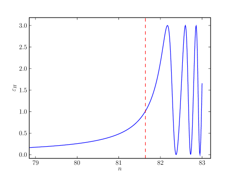
The background system requires initial conditions for ${\varphi}_{0},\dot{{\varphi}_{0}}$ and $H$. These initial conditions and the range of e-foldings to be simulated must be selected with the choice of potential in mind. Not only must the e-folding range include an inflationary period, but the $k$ modes to be calculated at first and second order must begin inside the horizon during this range. For example the initial conditions ${\varphi}_{0}=18M_{\mathrm{PL}},\dot{{\varphi}_{0}}=-1M_{\mathrm{PL}},H=4.65{\times 10^{-5}}M_{\mathrm{PL}}$ for the $\frac{1}{2}m^{2}\varphi^{2}$ model give the background evolution described below and shown in Figure 1.

The initial conditions are set for each $k$ mode a few e-foldings before horizon crossing. This follows the example of Salopek et al. Salopek:1988qh and is justified on the basis that the mode is sufficiently inside the horizon for the Minkowski limit to be taken. This initial time, $n_{\mathrm{init}}(k)$, is calculated to be when

$$\frac{k}{aH|_{\mathrm{init}}}=50\,.$$ (34)

The range of e-foldings being used must include the starting point for all $k$ modes, but the parameter on the right hand side, here chosen to be 50, can be changed if needed. We use the small wavelength solution of the first order equations as the initial conditions Salopek:1988qh , with

$${\delta\varphi_{1}}|_{\mathrm{init}} = \frac{\sqrt{8\pi G}}{a}\frac{e^{-ik\eta}}{\sqrt{2k}}\,,$$ (35)

$$\dot{{\delta\varphi_{1}}}|_{\mathrm{init}} = -\frac{\sqrt{8\pi G}}{a}\frac{e^{-ik\eta}}{\sqrt{2k}}\left(1+i\frac{k}{aH}\right)\,,$$ (36)

where the conformal time $\eta$ can be calculated from $\eta=\int dn/aH\simeq-(aH(1-\epsilon_{H}))^{-1}$, when $\epsilon_{H}$ changes slowly. For example $k_{\mathrm{WMAP}}$ is initialised about $65$ e-foldings before the end of inflation and crosses the horizon about $5$ e-foldings later. We also use these formulae in the calculation of the source term in Eq. (30) to determine the value of ${\delta\varphi_{1}}$ for a $k$ mode before its evolution starts.

We are interested in the production of second order effects by the evolution of the the gaussian first order modes and we make no assumptions about the existence of second order perturbations before the simulation begins. Therefore we set the initial condition for each second order perturbation mode to be ${\delta\varphi_{2}}=0,\dot{{\delta\varphi_{2}}}=0$ at the time when the corresponding first order perturbation is initialised.

III.3 Implementation

The current implementation of the code is mainly in Python and uses the Numerical and Scientific Python modules for their strong compiled array support scipy . The core of the model computation is a customised Runge-Kutta 4th order method (see for example Eq. (25.5.10) in abramowitz+stegun ). Following Refs. Martin:2006rs ; Ringeval:2007am the numerical calculation proceeds in four stages. The background equation (27), rewritten as two first order (in the time derivative) equations, is evolved from the specified initial state until some end time required to be after the end of the inflationary regime. The end of inflation occurs when $d^{2}a/dt^{2}$ is no longer positive and the parameter $\varepsilon_{H}=-\dot{H}/H$ first becomes greater than or equal to $1$ (see Figure 1). Here, this specifies a new end time for the 1st order run, although the simulation can run beyond the strict end of inflation if required. The initial conditions for the first order system are then set as outlined above.

Figure 1: The end of inflation is determined by calculating when $\varepsilon_{H}=-\dot{H}/H=1$ (red dashed line). Along the $x$-axis, $n$ is the number of e-foldings from the start of the simulation.

The system of ordinary differential equations for the first order perturbations from Eq. (28) is calculated using a standard Runge-Kutta method. A fixed time step method is used in order to simplify the construction of the second order source term and because a priori it is not known which time steps would be required at second order if an adaptive time step system were used. The first order equations are separable in terms of $k$ and so it is straightforward to run multiple instances of the system and collate the results at the end. However, as will be discussed below, the first order calculation is not computationally expensive in comparison with the other stages and takes of the order of a few minutes for around $8000$ time steps and $1025$ $k$ modes.

Once the first order system has been solved the source term for the second order system must be calculated. As the real space equation for the source involves terms quadratic in the first order perturbation it is necessary to perform a convolution in Fourier space, as shown in Eq. (22). Transforming back into real space was not considered due to the presence of both gradient operators and their inverses. Here the slow roll version of the source term integrand has been used, but the method can equally be applied to the full equation. This stage is the most computationally intensive and can be run in parallel as each time step is independent of the others. The nature of the convolution integral and the dependence of the first order perturbation on the absolute value of its arguments requires that twice as many $k$ modes are calculated at first order than are desired at second order as explained above. As the first order calculation is computationally cheaper than the source term integration, this does not significantly lower the possible resolution in $k$-space, which is still limited by the source term computation time. Once the integrand is determined it is fed into a Romberg integration scheme. As for $\theta$ which was discretised by $N_{\theta}$ points in Eq. (III.1), this requires that the number of $k$ modes is

$$N_{k}=2^{l}+1\,,$$ (37)

for some$l\in\mathbb{N}$. This requirement can be lifted by opting for a less accurate and somewhat slower standard quadrature routine.

The second order system is finally run with the source term and other necessary data being read as required from the memory or disk. The Runge-Kutta method calculates half time steps for each required point, for example if $y(x_{n})$ is known and $y(x_{n+1})=y(x_{n}+h)$ is required (for step size $h$), the method will calculate the derivatives of $y$ at $y(x_{n}),y(x_{n}+h/2)$ and $y(x_{n}+h)$. As we need to specify the source term at every calculated timestep, the requested timestep for the second order method must be twice that used at first order. This decreases the accuracy of the method but does not require the use of splines and interpolation techniques to determine background and 1st order variables between time steps.

The second order system is similar in run time to the first order system but the source integration is more complex, involving the integration of $N_{k}^{2}\times N_{\theta}$ values at each time step. Although a large amount of data is produced at each step at this stage for each of the wavenumbers $k$, only the integrated result is stored to be used in the second order run. Results for each stage are stored in the open HDF5 standard which can deal efficiently with large files and is very portable, allowing data analysis independent of the Python/Numpy programming environment. We intend to release the program under a suitable license once the code has matured and some of the improvements discussed in Section V have been implemented.

III.4 Code Tests

We have tested the numerical code in a variety of controlled circumstances in order to quantify the effect of different choices of parameters. In particular it is important to know whether the values picked for $N_{\theta}$, the number of discretised $\theta$s, $\Delta k$, the size of the spacing of the discretised $k$ modes, and the range of $k$ values significantly impacts on the results. The ODE solving parts of the code are straightforward and follow standard algorithms.

As mentioned above the WMAP results Komatsu:2008hk use observations in the range $k\in[0.92{\times 10^{-60}},3.1\times 10^{-58}]M_{\mathrm{PL}}=[3.5{\times 10^{-4}},0.12]M_{\mathrm{pc}}^{-1}$. We will consider three different $k$ ranges both in our results and the tests of the code:

$$K_{1} = \left[1.9{\times 10^{-5}},0.039\right]M\mathrm{pc}^{-1}\,,\quad\Delta k=3.8{\times 10^{-5}}M\mathrm{pc}^{-1}\,,$$

$$K_{2} = \left[5.71{\times 10^{-5}},0.12\right]M\mathrm{pc}^{-1}\,,\quad\Delta k=1.2{\times 10^{-4}}M\mathrm{pc}^{-1}\,,$$

$$K_{3} = \left[0.52{\times 10^{-5}},0.39\right]M\mathrm{pc}^{-1}\,,\quad\Delta k=3.8{\times 10^{-4}}M\mathrm{pc}^{-1}\,.$$ (38)

The first, $K_{1}$, has a very fine resolution but covers only a small portion of the WMAP range. The next, $K_{2}$, is closest to the WMAP range with a still quite fine resolution. The final range, $K_{3}$, has a larger $k$ mode step size $\Delta k=1{\times 10^{-60}}M_{\mathrm{PL}}=3.8{\times 10^{-4}}M\mathrm{pc}^{-1}$ and covers a greater range than the others, extending to much smaller scales than WMAP can observe.

(a) The relative error for different $N_{\theta}$, the number of discretised $\theta$s, keeping the other parameters fixed and using the $K_{3}$ range. The upper blue line ($N_{\theta}=129$) and middle green line ($N_{\theta}=257$) have relative errors at least an order of magnitude larger than the lower red line ($N_{\theta}=513$).

(b) The relative error for the 3 different $k$ ranges $K1$, $K2$, $K3$ (starting from the left). The parameter $\Delta k$ is set equal to $1{\times 10^{-61}}M_{\mathrm{PL}},3{\times 10^{-61}}M_{\mathrm{PL}},1{\times 10^{-60}}M_{\mathrm{PL}}$ respectively.

Figure 2: Comparison of relative errors for different $N_{\theta}$ and $k$ ranges.

The main new addition in the code is the calculation of the convolution of the perturbations for the source term Eq. (30). In particular the first of the $\theta$ dependent terms in Eq. (III.1), $A$, can be convolved analytically for certain smooth ${\delta\varphi_{1}}(k)$s. We take ${\delta\varphi_{1}}(k)$ to be similar in form to the initial conditions (35), for example ${\delta\varphi_{1}}(k)\propto 1/\sqrt{k}$ with proportionality constant $\alpha$. If $I_{A}$ denotes the convolution of the $A$ term:

$$I_{A}(k)=2\pi\int_{k_{\mathrm{min}}}^{k_{\mathrm{max}}}q^{2}{\delta\varphi_{1}}(q)A(k,q)dq\,,$$ (39)

then putting in ${\delta\varphi_{1}}(k)=\alpha/\sqrt{k}$ gives

$$I_{A}(k)=2\pi\alpha^{2}\int_{k_{\mathrm{min}}}^{k_{\mathrm{max}}}dq\,q^{\frac{3}{2}}\int_{0}^{\pi}d\theta\,(k^{2}+q^{2}-2kq\cos{\theta})^{-4}\sin{\theta}\,.$$ (40)

This has the analytic solution

$$A(k) = \frac{\pi}{18}\frac{\alpha^{2}}{k}\left\{3k^{3}\left[\log\left(2\sqrt{k}\right)-\frac{\pi}{2}+\arctan\left(\sqrt{\frac{k_{\mathrm{min}}}{k-k_{\mathrm{min}}}}\right)+\log\left(2\left(\sqrt{k_{\mathrm{min}}}+\sqrt{k_{\mathrm{min}}+k}\right)\right)\right.\right.$$ (41)

$$\left.-\,\log\left(2\left(\sqrt{k_{\mathrm{max}}}+\sqrt{k_{\mathrm{max}}+k}\right)\right)-\log\left(2\left(\sqrt{k_{\mathrm{max}}}+\sqrt{k_{\mathrm{max}}-k}\right)\right)\right]$$

$$+\,\sqrt{k_{\mathrm{max}}}\left[\sqrt{k_{\mathrm{max}}-k}\left(-3k^{2}+14kk_{\mathrm{max}}-8k_{\mathrm{max}}^{2}\right)+\sqrt{k_{\mathrm{max}}+k}\left(3k^{2}+14kk_{\mathrm{max}}+8k_{\mathrm{max}}^{2}\right)\right]$$

$$\left.-\,\sqrt{k_{\mathrm{min}}}\left[\sqrt{k-k_{\mathrm{min}}}\left(3k^{2}-14kk_{\mathrm{max}}+8k_{\mathrm{max}}^{2}\right)-\sqrt{k+k_{\mathrm{min}}}\left(3k^{2}+14kk_{\mathrm{max}}+8k_{\mathrm{max}}^{2}\right)\right]\right\}\,.$$

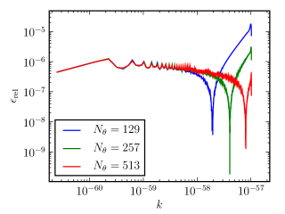
We have tested our code against this analytic solution for various combinations of $k$ ranges and $N_{\theta}$. The relative error

$$\epsilon_{\mathrm{rel}}=\frac{|\mathrm{analytic}-\mathrm{calculated}|}{|\mathrm{analytic}|}$$ (42)

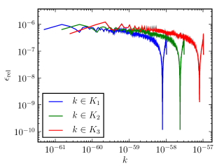
is small for all the tested cases but certain combinations of parameters turned out to be better than others. The relative error of all the following results is not affected by the choice of $\alpha$ so we will keep it constant throughout.

Figure 3: The relative error in convolution term $A$ for different values of $\Delta k$. The other parameters are fixed: $k_{\mathrm{min}}=1\times 10^{-60}M_{\mathrm{PL}},N_{k}=1025$ and $N_{\theta}=513$. The upper blue line ($\Delta k=1{\times 10^{-61}}M_{\mathrm{PL}}$ and middle green line ($\Delta k=3{\times 10^{-61}}M_{\mathrm{PL}}$) have relative errors at least an order of magnitude larger than the lower red line ($\Delta k=1{\times 10^{-60}}M_{\mathrm{PL}}$).

We first tested the effect of changing $N_{\theta}$, the number of samples of the $\theta$ range $[0,\pi]$. Figure 2(a) plots these results for the $k$ range $K_{3}$ with $\Delta k=1{\times 10^{-60}}M_{\mathrm{PL}}$. Only three values of $N_{\theta}$ are shown for clarity. It can be seen that increasing $N_{\theta}$ decreases the relative error (for the convolution term at least) when the other parameters are kept constant, as one might expect.

As mentioned above the choice of $k$ range is especially important as the convolution of the terms depends heavily on the minimum and maximum values of this range. Indeed this is clear from the analytic solution in Eq. (41). Figure 2(b) shows the difference in relative error for the three different $k$ ranges described above with $\Delta k=3.8{\times 10^{-5}},1.2{\times 10^{-4}}$ and $3.8{\times 10^{-4}}M\mathrm{pc}^{-1}$ ($\Delta k=1{\times 10^{-61}},3{\times 10^{-61}},1{\times 10^{-60}}M_{\mathrm{PL}}$) respectively. The accuracy is similar in all three cases.

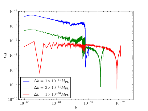
Another important check is whether the resolution of the $k$ range is fine enough. Varying $\Delta k$ can not be done in isolation of course, if the constraint for $N_{k}$, Eq. (37), is to be met. For this test the end of the $k$ range changed with $\Delta k$ but the other parameters were kept fixed as $k_{\mathrm{min}}=1{\times 10^{-60}}M_{\mathrm{PL}}=3.8{\times 10^{-4}}M\mathrm{pc}^{-1},N_{k}=1025$ and $N_{\theta}=513$. Figure 3 plots these results again for only three indicative values. For $\Delta k<k_{\mathrm{min}}$, here the upper two lines, there is a marked degradation in the accuracy of the method. This is understandable as many interpolations of multiples of $\Delta k$ below $k_{\mathrm{min}}$ will be set to $0$. Once $\Delta k$ is greater than $k_{\mathrm{min}}$ the relative error is very similar for higher values (not shown in the figure).

Figure 4: The relative error of the convolution term for three different values of $\Delta k$. In contrast to Figure 3 $k_{\mathrm{min}}=1{\times 10^{-61}}M_{\mathrm{PL}}=3.8{\times 10^{-5}}M\mathrm{pc}^{-1}\leq\Delta k$ for each.

It should be noted that these tests show the relative errors in the computation of the $A$ convolution term, the most straightforward term in Eq. (III.1), only and do not represent errors for the full calculation. However, they show that at least for the pure convolution term the accuracy is good compared with the analytic results. Equation (41) gives some indication of the difficulty involved in finding an analytic solution for the other terms, although this is a goal for future work. Having described the implementation and accuracy of the numerical system we will outline our results in the next section.

IV Results

The main result of this paper is the demonstration of a numerical solution to the closed Klein-Gordon equation of motion for second order scalar field perturbations as described in Eq. (19). This includes the slow roll approximation of the source term for second order perturbations, but we have not used a slow roll version of the evolution equations for the background or first order perturbations.

As a proof of concept we have tested the system with two standard potentials, $\frac{1}{2}m^{2}\varphi^{2}$ and $\frac{1}{4}\lambda\varphi^{4}$ and computed results across three different $k$ ranges. As expected, considering the use of a single slowly rolling field, the second order perturbation we have calculated is extremely small in comparison with the first order term. However there are already differences apparent between the two potentials which will be outlined below. We have calibrated the parameters $m$ and $\lambda$ of the potentials using the WMAP 5 normalisation at $k_{\mathrm{WMAP}}=0.002M\mathrm{pc}^{-1}=5.25{\times 10^{-60}}M_{\mathrm{PL}}$ Komatsu:2008hk . We have outlined in Eq. (III.4) the three $k$ ranges that we will use,

$$K_{1} = \left[1.9{\times 10^{-5}},0.039\right]M\mathrm{pc}^{-1}\,,\quad\Delta k=3.8{\times 10^{-5}}M\mathrm{pc}^{-1}$$

$$K_{2} = \left[5.71{\times 10^{-5}},0.12\right]M\mathrm{pc}^{-1}\,,\quad\Delta k=1.2{\times 10^{-4}}M\mathrm{pc}^{-1}$$

$$K_{3} = \left[0.52{\times 10^{-5}},0.39\right]M\mathrm{pc}^{-1}\,,\quad\Delta k=3.8{\times 10^{-4}}M\mathrm{pc}^{-1}\,.$$

Many of the results will be quoted for $k_{\mathrm{WMAP}}$ which lies in all three of these ranges.

Given that the first order perturbations for the chosen potentials give an almost scale invariant power spectrum with no running, it is no surprise that the results from the three different $k$ ranges are very similar. The second order source term is somewhat dependent on the lower bound of $k$ (upper bound on size). This is expected and in the scale invariant case a log divergence can be shown to exist Lyth:2007jh . We have implemented an arbitrary sharp cutoff at $k_{\mathrm{min}}$ below which ${\delta\varphi_{1}}$ is taken to be zero. As mentioned above there is some evidence to suggest that a similar cutoff is supported by the WMAP data Sinha:2005mn ; Kim:2009pf .

At first order our solutions agree with previous work Salopek:1988qh ; Martin:2006rs ; Ringeval:2007am , with oscillations being damped until horizon crossing (when $k=aH$) after which the curvature perturbation becomes conserved. Figure 5 shows the real and imaginary parts of the first order perturbations from when the initial conditions are set at $k/aH=50$ to just after horizon crossing. The x-axis for most of the following figures shows the number of e-foldings left until the end of inflation instead of the internally used time variable $n$.

Figure 5: The first order perturbation ${\delta\varphi_{1}}$ rescaled by $k^{3/2}/(\sqrt{2}\pi)$ from the beginning of the simulation until around horizon crossing (red dot-dashed line). The real (blue) and imaginary (green dashed) perturbations are shown for $k_{\mathrm{WMAP}}$.

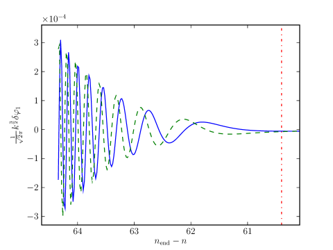
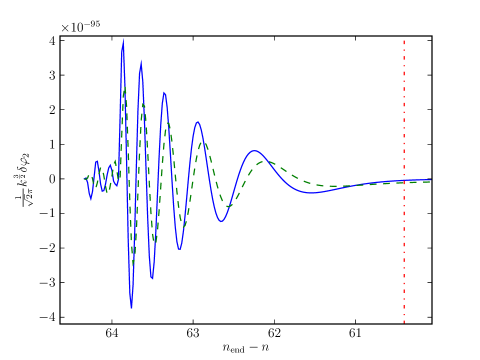
In Figure 6 we show the evolution of the second order perturbations for wavenumber $k_{\mathrm{WMAP}}$. As mentioned above the overall amplitude of the second order perturbations is many orders of magnitude smaller than the first order ones. In Figures 5 and 6 the field values have been rescaled by $k^{3/2}/(\sqrt{2}\pi)$ to allow a better appreciation of the magnitude of the resulting power spectra.

Figure 6: The real (blue line) and imaginary (green dashed) components of the second order perturbation ${\delta\varphi_{2}}(k_{\mathrm{WMAP}})$ from the beginning of the simulation until around the time of horizon exit (red dot-dashed line).

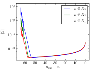
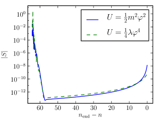
The source term $S({{k^{i}}})$ is calculated at each time step using the results of the first order and background runs. This term drives the production of second order perturbations as shown in Eqs. (19) and (29). Figure 7(a) shows the absolute magnitude of the source term for a single $k$ mode, $k_{\mathrm{WMAP}}$, for all time steps calculated.

(a) Absolute magnitude of the source term.

(b) Power spectrum of scalar perturbations $\mathcal{P}_{\delta\varphi}=\frac{k^{3}}{2\pi^{2}}|\delta\varphi|^{2}$.

Figure 7: Source term and power spectrum for the WMAP pivot scale $k_{\mathrm{WMAP}}$.

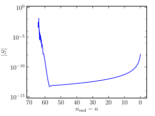
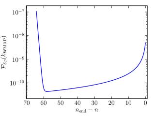
Figure 8(a) shows how the source term changes with the choice of $k$ range. After horizon crossing the source terms are approximately equal. Before horizon crossing however there is a strict hierarchy with the smaller $k$ ranges, $K_{1}$ and $K_{2}$, leading to smaller source contributions. As stated in Section III.4, $\Delta k$ should be at least as large as $k_{\mathrm{min}}$ in order to reduce the error to a minimum.

(a) Comparison of the source term for $k_{\mathrm{WMAP}}$ over three different ranges with different $\Delta k$s as specified in Eq. (III.4).

(b) The source term for three different $k$ values including the WMAP pivot scale. As $k$ gets larger (scale gets smaller) the source term becomes smaller.

Figure 8: Two different comparisons of the source term $S$.

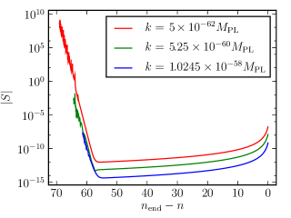
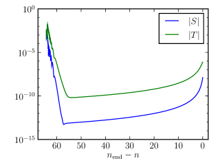
The source term is large at early times, and closely follows the form of the spectrum of the first order perturbations as can be seen from Figure 7(b). It is useful to compare the magnitude of the source term with the other terms in the second order evolution equation (29). If we let $T$ denote the other terms,

$$T({{k^{i}}})=\left(3+\frac{\dot{H}}{H}\right)\dot{{\delta\varphi_{2}}}({{k^{i}}})+\left(\frac{k}{aH}\right)^{2}{\delta\varphi_{2}}({{k^{i}}})+\left(\frac{U_{,\varphi\varphi}}{H^{2}}-{24\pi G}(\dot{{\varphi}_{0}})^{2}\right){\delta\varphi_{2}}({{k^{i}}})\,,$$ (43)

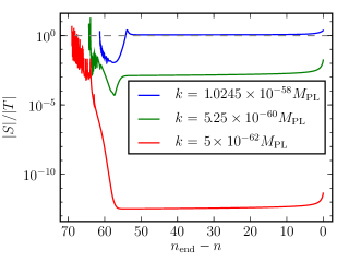
then Figure 9(a) shows the absolute magnitude of both $S$ and $T$. It is clear that the source term is of comparable magnitude only early in the simulation. Figure 9(b) shows a comparison of $|S|/|T|$ for three different $k$ values. The larger the $k$ mode the closer in amplitude $S$ is to the rest of the terms in the ODE. A priori it is not known where $S$ will be large for a particular chosen potential and mode but once determined it could be possible to significantly reduce the time required for the simulation by only calculating $S$ in the regions where it is important.

(a) The source term (lower blue line) is compared with the $T$ term (upper green line) as defined in the text for $k_{\mathrm{WMAP}}$. The source term is of comparable magnitude at the beginning of the simulation.

(b) The quotient of $S$ and $T$ terms for three different $k$ values including the WMAP pivot scale. Depending on $k$ the source term only dominates at early stages or is important throughout the evolution.

Figure 9: Source term $S$ compared with $T$.

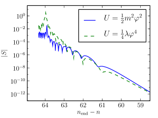
All the results quoted so far are for the $\frac{1}{2}m^{2}\varphi^{2}$ model. We have also tested the $\frac{1}{4}\lambda\varphi^{4}$ model and compared it to $\frac{1}{2}m^{2}\varphi^{2}$. Figure 10 compares the models for $k_{\mathrm{WMAP}}$. Figure 10(b) shows how the source term for the $\frac{1}{4}\lambda\varphi^{4}$ model is larger than the one for $\frac{1}{2}m^{2}\varphi^{2}$ to begin, but crosses over after a few e-foldings. After horizon crossing the $\frac{1}{4}\lambda\varphi^{4}$ source term is again larger. As the results at first order for both models are so similar it is to be expected that the second order perturbations would be closely related.

(a) The $\frac{1}{4}\lambda\varphi^{4}$ model (green dashed line) initially has a larger source term but becomes smaller than the $\frac{1}{2}m^{2}\varphi^{2}$ model as evolution continues. After horizon crossing the $\frac{1}{4}\lambda\varphi^{4}$ term is slightly larger.

(b) The crossover between the models at the early stages of the simulation, before horizon crossing.

Figure 10: A comparison of the source term for the $\frac{1}{2}m^{2}\varphi^{2}$ and $\frac{1}{4}\lambda\varphi^{4}$ models.

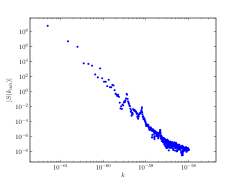
In Figure 11 the value of $|S|$ at the start of the evolution of ${\delta\varphi_{2}}$ for each $k$ mode is shown. The magnitude of the source term is much smaller for larger $k$s (smaller scales). Because the smaller $k$s begin their evolution earlier the relative difference in $|S|$ is not as pronounced when measured at a single timestep (see for example Figure 8(b)). It should also be remembered that the magnitude of other terms in the second order ODE is small for larger $k$s as shown by the ratio $|S|/|T|$ in Figure 9 where $T$ is defined above in Eq. (43).

Figure 11: The absolute magnitude of the source term at the initial start time for each $k$ when $k=aH\times 50$ deep inside the horizon. The results are for the range $K_{1}=\left[1.9{\times 10^{-5}},0.039\right]M\mathrm{pc}^{-1}=\left[0.5{\times 10^{-61}},1.0245{\times 10^{-58}}\right]M_{\mathrm{PL}}$.

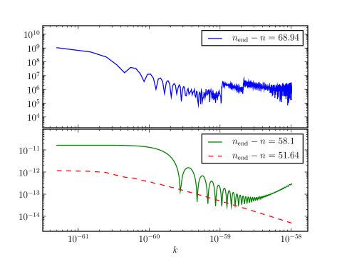
The source term for all $k$s can also be compared for different timesteps. In Figure 12 the upper blue line shows $|S(k)|$ around 69 e-foldings before the end of inflation when ${\delta\varphi_{2}}$ has been initialised for only the very smallest $k$ modes. The middle green line shows $|S|$ when all ${\delta\varphi_{2}}$ modes have been started. Finally the lower red line plots $|S|$ after all modes have exited the horizon, around 52 e-foldings before the end of inflation.

Figure 12: The absolute magnitude of the source term for all $ks$ in the range at three different timesteps: the upper blue line when only the largest modes have been initialised; the middle green line when all modes have been initialised; and the lower red dashed line when all modes have exited the horizon. The $k$ range shown here is $K_{1}=\left[1.9{\times 10^{-5}},0.039\right]M\mathrm{pc}^{-1}=\left[0.5{\times 10^{-61}},1.0245{\times 10^{-58}}\right]M_{\mathrm{PL}}$.

V Discussion and conclusion

In this paper we have described the numerical solution of the evolution equations for second order scalar perturbations, using the closed form of the Klein-Gordon equation, Eq. (19). We demonstrate that direct calculation of field perturbations beyond first order using perturbation theory is readily achievable, though not trivial.

For this first demonstration we have limited ourselves to considering the slow roll source term in Eq. (19) but without imposing slow roll on the evolution terms of the ODEs. We have investigated two standard potentials, $\frac{1}{2}m^{2}\phi^{2}$ and $\frac{1}{4}\lambda\phi^{4}$, to demonstrate the capabilities of the system. The singularity at $k=0$ which arises as larger and larger scales are considered is avoided by implementing a cutoff at small wavenumbers below $k_{\mathrm{min}}$. This is a pragmatic choice necessary for the calculation, but as mentioned above there is some evidence that such a cutoff might also explain lack of power at large scales in the WMAP data spergel ; Sinha:2005mn ; Kim:2009pf . It is also necessary to pick a maximum $k$ value, and this choice is dictated by computational resources and with reference to observationally relevant scales. In this paper we have used $k$ ranges which are comparable with the scales observed by WMAP. By comparing the analytical results of the convolution integral with the numerical calculation, we have chosen values of the parameters $N_{\theta},N_{k}$ and $\Delta k$ which minimise the numerical error. The convolution scheme that we have implemented works best when $\Delta k>k_{\mathrm{min}}$.

We have shown explicitly that the second order calculations for our chosen potentials are obtainable once the cut-off for $k_{\mathrm{min}}$ is implemented. As expected for these unexceptional potentials in the slowly rolling regime the magnitude of second order perturbations is extremely suppressed in comparison with the first order amplitude. We have shown the evolution of the source term equation during the inflationary regime can be readily calculated.

There are many possible next steps to improve the program outlined in Section III. Chief amongst these is to implement the full source term equation (30). Although clearly more complicated than the slow roll case in Eq. (29) only two more $\theta$ dependent terms need to be added to $A$–$D$ in Eq. (III.1). For the two test models we have used in this paper, which are both slowly rolling during inflation, it is not expected that using the full source equation would result in an appreciably different outcome until the end of the inflationary phase. Though once the field has stopped to roll slowly, new observable features might arise as is indeed the case at first order.

Beyond this the next likely step is to implement a multi-field version of the system. This would allow the investigation of models that inherently produce large second order perturbations. In Ref. Malik:2006ir the Klein-Gordon equation is given for multiple fields and upgrading the simulation to use these equations is a straight-forward if lengthy process.

The performance of the numerical simulation could also be improved by analysing the most time consuming processes and investigating what optimisations could be implemented. As we have discussed above we have set $N_{k}=1025$ for our test runs. This provides good coverage of the WMAP $k$ range but it is not clear whether it sufficiently approximates the integral to infinity for the source term. Currently we are restricted in our choice of $N_{k}$ by logistical factors i.e. the running time and memory usage of the code. By optimising the routines for both memory and speed it is hoped we can extend the maximum value of $k$ to larger values.

By computing the perturbations to second order we have direct access to the non-gaussianity of ${\delta\varphi}$. While useful for the toy models discussed above (with $f_{\mathrm{NL}}\simeq 0$), when used to investigate models with predictions of large non-linearity parameter $f_{\mathrm{NL}}$ this technique could yield greater insight into the formation and development of the non-gaussian contributions by studying the contribution of the different terms in the source term Eq. (30). It was shown recently that in order to calculate $f_{\mathrm{NL}}$ instead of using the standard method based on the Lagrangian formalism Maldacena:2002vr , one can instead use the field equations Musso:2006pt ; Seery:2008qj . The method presented here will therefore eventually allow a full numerical calculation of $f_{\mathrm{NL}}$.

In summary, we have demonstrated that numerically solving the closed Klein-Gordon equation for second order perturbations is possible. We have used the slow roll version of the source term in this paper, but hope to extend our work to use the full source soon. The two test models we have used have been shown to have negligible second order perturbations in line with analytic results. We have compared the analytic and numerical solutions for the convolution term and found them to be in good agreement.

References

- (1) “Planck Project .” http://www.rssd.esa.int/index.php?project=Planck.
- (2) WMAP Collaboration, E. Komatsu et al., “Five-Year Wilkinson Microwave Anisotropy Probe (WMAP) Observations:Cosmological Interpretation,” Astrophys. J. Suppl. 180 (2009) 330–376, arXiv:0803.0547 [astro-ph].
- (3) D. S. Salopek and J. R. Bond, “Nonlinear evolution of long wavelength metric fluctuations in inflationary models,” Phys. Rev. D42 (1990) 3936–3962.
- (4) G. I. Rigopoulos, E. P. S. Shellard, and B. J. W. van Tent, “Non-linear perturbations in multiple-field inflation,” Phys. Rev. D73 (2006) 083521, arXiv:astro-ph/0504508.
- (5) A. A. Starobinsky, “Dynamics of Phase Transition in the New Inflationary Universe Scenario and Generation of Perturbations,” Phys. Lett. B117 (1982) 175–178.
- (6) A. A. Starobinsky, “Multicomponent de Sitter (Inflationary) Stages and the Generation of Perturbations,” JETP Lett. 42 (1985) 152–155. [Pisma Zh. Eksp. Teor. Fiz. 42 (1985) 124].
- (7) M. Sasaki and E. D. Stewart, “A General analytic formula for the spectral index of the density perturbations produced during inflation,” Prog. Theor. Phys. 95 (1996) 71–78, arXiv:astro-ph/9507001.
- (8) M. Sasaki and T. Tanaka, “Super-horizon scale dynamics of multi-scalar inflation,” Prog. Theor. Phys. 99 (1998) 763–782, arXiv:gr-qc/9801017.
- (9) D. H. Lyth, K. A. Malik, and M. Sasaki, “A general proof of the conservation of the curvature perturbation,” JCAP 0505 (2005) 004, arXiv:astro-ph/0411220.
- (10) D. H. Lyth and Y. Rodriguez, “The inflationary prediction for primordial non- gaussianity,” Phys. Rev. Lett. 95 (2005) 121302, arXiv:astro-ph/0504045.
- (11) D. Langlois and F. Vernizzi, “Nonlinear perturbations of cosmological scalar fields,” JCAP 0702 (2007) 017, arXiv:astro-ph/0610064.
- (12) J. M. Bardeen, “Gauge Invariant Cosmological Perturbations,” Phys. Rev. D22 (1980) 1882–1905.
- (13) K. Tomita, “Non-Linear Theory of Gravitational Instability in the Expanding Universe,” Progress of Theoretical Physics 37 (1967) 831–846.
- (14) V. F. Mukhanov, L. R. W. Abramo, and R. H. Brandenberger, “On the back reaction problem for gravitational perturbations,” Phys. Rev. Lett. 78 (1997) 1624–1627, arXiv:gr-qc/9609026.
- (15) M. Bruni, S. Matarrese, S. Mollerach, and S. Sonego, “Perturbations of spacetime: Gauge transformations and gauge invariance at second order and beyond,” Class. Quant. Grav. 14 (1997) 2585–2606, arXiv:gr-qc/9609040.
- (16) V. Acquaviva, N. Bartolo, S. Matarrese, and A. Riotto, “Second-order cosmological perturbations from inflation,” Nucl. Phys. B667 (2003) 119–148, arXiv:astro-ph/0209156.
- (17) K. Nakamura, “Gauge invariant variables in two-parameter nonlinear perturbations,” Prog. Theor. Phys. 110 (2003) 723–755, arXiv:gr-qc/0303090.
- (18) H. Noh and J.-c. Hwang, “Second-order perturbations of the Friedmann world model,” Phys. Rev. D69 (2004) 104011.
- (19) F. Bernardeau and J.-P. Uzan, “Non-Gaussianity in multi-field inflation,” Phys. Rev. D66 (2002) 103506, arXiv:hep-ph/0207295.
- (20) J. M. Maldacena, “Non-Gaussian features of primordial fluctuations in single field inflationary models,” JHEP 05 (2003) 013, arXiv:astro-ph/0210603.
- (21) F. Finelli, G. Marozzi, G. P. Vacca, and G. Venturi, “Energy-momentum tensor of cosmological fluctuations during inflation,” Phys. Rev. D69 (2004) 123508, arXiv:gr-qc/0310086.
- (22) N. Bartolo, E. Komatsu, S. Matarrese, and A. Riotto, “Non-Gaussianity from inflation: Theory and observations,” Phys. Rept. 402 (2004) 103–266, arXiv:astro-ph/0406398. http://dx.doi.org/10.1016/j.physrep.2004.08.022.
- (23) K. Enqvist and A. Vaihkonen, “Non-Gaussian perturbations in hybrid inflation,” JCAP 0409 (2004) 006, arXiv:hep-ph/0405103.
- (24) D. H. Lyth and Y. Rodriguez, “Non-gaussianity from the second-order cosmological perturbation,” Phys. Rev. D71 (2005) 123508, arXiv:astro-ph/0502578.
- (25) D. Seery and J. E. Lidsey, “Primordial non-gaussianities from multiple-field inflation,” JCAP 0509 (2005) 011, arXiv:astro-ph/0506056.
- (26) K. A. Malik and D. Wands, “Evolution of second order cosmological perturbations,” Class. Quant. Grav. 21 (2004) L65–L72, arXiv:astro-ph/0307055.
- (27) N. Barnaby and J. M. Cline, “Nongaussian and nonscale-invariant perturbations from tachyonic preheating in hybrid inflation,” Phys. Rev. D73 (2006) 106012, arXiv:astro-ph/0601481.
- (28) K. A. Malik and D. Wands, “Cosmological perturbations,” Phys. Rept. 475 (2009) 1–51, arXiv:0809.4944 [astro-ph].
- (29) K. A. Malik, “Gauge-invariant perturbations at second order: Multiple scalar fields on large scales,” JCAP 0511 (2005) 005, arXiv:astro-ph/0506532.
- (30) K. A. Malik, “A not so short note on the Klein-Gordon equation at second order,” JCAP 0703 (2007) 004, arXiv:astro-ph/0610864.
- (31) F. Finelli, G. Marozzi, G. P. Vacca, and G. Venturi, “Second order gauge-invariant perturbations during inflation,” Phys. Rev. D74 (2006) 083522, arXiv:gr-qc/0604081.
- (32) M. Sasaki, “Large Scale Quantum Fluctuations in the Inflationary Universe,” Prog. Theor. Phys. 76 (1986) 1036.
- (33) V. F. Mukhanov, “Quantum Theory of Gauge Invariant Cosmological Perturbations,” Sov. Phys. JETP 67 (1988) 1297–1302.
- (34) A. Vretblad, Fourier Analysis and Its Applications (Graduate Texts in Mathematics). Springer, 2005.
- (35) A. R. Liddle and D. H. Lyth, Cosmological Inflation and Large-Scale Structure. Cambridge University Press, April, 2000.
- (36) J. Martin and C. Ringeval, “Inflation after WMAP3: Confronting the slow-roll and exact power spectra to CMB data,” JCAP 0608 (2006) 009, arXiv:astro-ph/0605367.
- (37) C. Ringeval, “The exact numerical treatment of inflationary models,” Lect. Notes Phys. 738 (2008) 243–273, arXiv:astro-ph/0703486.
- (38) D. S. Salopek, J. R. Bond, and J. M. Bardeen, “Designing Density Fluctuation Spectra in Inflation,” Phys. Rev. D40 (1989) 1753.
- (39) D. H. Lyth, “The curvature perturbation in a box,” JCAP 0712 (2007) 016, arXiv:0707.0361 [astro-ph].
- (40) WMAP Collaboration, D. N. Spergel et al., “Wilkinson Microwave Anisotropy Probe (WMAP) three year results: Implications for cosmology,” Astrophys. J. Suppl. 170 (2007) 377, arXiv:astro-ph/0603449.
- (41) R. Sinha and T. Souradeep, “Post-WMAP assessment of infrared cutoff in the primordial spectrum from inflation,” Phys. Rev. D74 (2006) 043518, arXiv:astro-ph/0511808.
- (42) J. Kim and P. Naselsky, “The primordial ’’ non-Gaussianity, and perturbations beyond the present horizon,” Phys. Rev. D79 (2009) 123006, arXiv:0905.1781 [astro-ph.CO].
- (43) H. V. Peiris and R. Easther, “Primordial Black Holes, Eternal Inflation, and the Inflationary Parameter Space after WMAP5,” JCAP 0807 (2008) 024, arXiv:0805.2154 [astro-ph].
- (44) E. Jones, T. Oliphant, P. Peterson, et al., “SciPy: Open source scientific tools for Python.” http://www.scipy.org/, 2001–.
- (45) M. Abramowitz and I. A. Stegun, Handbook of Mathematical Functions with Formulas, Graphs, and Mathematical Tables. Dover, New York, 1964.
- (46) M. Musso, “A new diagrammatic representation for correlation functions in the in-in formalism,” arXiv:hep-th/0611258.
- (47) D. Seery, K. A. Malik, and D. H. Lyth, “Non-gaussianity of inflationary field perturbations from the field equation,” JCAP 0803 (2008) 014, arXiv:0802.0588 [astro-ph].