DESY 09-096 ISSN 0418-9833

October 2009

Measurement of the Charm and Beauty
Structure Functions using
the H1 Vertex Detector at HERA

H1 Collaboration

Inclusive charm and beauty cross sections are measured in $e^{-}p$ and $e^{+}p$ neutral current collisions at HERA in the kinematic region of photon virtuality $5\leq Q^{2}\leq 2000~{}{\rm GeV}^{2}$ and Bjorken scaling variable $0.0002\leq x\leq 0.05$. The data were collected with the H1 detector in the years 2006 and 2007 corresponding to an integrated luminosity of 189 ${\rm pb^{-1}}$. The numbers of charm and beauty events are determined using variables reconstructed by the H1 vertex detector including the impact parameter of tracks to the primary vertex and the position of the secondary vertex. The measurements are combined with previous data and compared to QCD predictions.

Accepted by Eur. Phys. J. C.

1 Introduction

The measurement of the inclusive charm ($c$) and beauty ($b$) quark cross sections and the derived structure functions $F_{2}^{c\bar{c}}$ and $F_{2}^{b\bar{b}}$ in DIS at HERA is an important test of the theory of the strong interaction, quantum chromodynamics (QCD), within the Standard Model. These measurements uniquely constrain the parton density functions (PDFs) of the proton, in particular its $b$ and $c$ content. Precise knowledge of the PDFs is for example essential at the Large Hadron Collider (LHC). The predictions of the ‘standard candle’ QCD processes at the LHC, such as the inclusive production of $W$ and $Z$ bosons, are sensitive to the theoretical treatment of heavy quarks [1, 2, 3, 4, 5, 6, 7]. The $b$ quark density is important in Higgs production at the LHC in both the Standard Model and in extensions to the Standard Model such as supersymmetric models at high values of the mixing parameter $\tan\beta$[8].

This paper reports on measurements made in neutral current deep inelastic scattering (DIS) at HERA of the charm and beauty contributions to the inclusive proton structure function $F_{2}$ in the range of virtuality of the exchanged photon $5\leq Q^{2}\leq 2000$ ${\rm GeV}^{2}$ and Bjorken $x$ $0.0002\leq x\leq 0.05$. The analysis uses the precise spatial information from the H1 vertex detector to separate events containing $c$ and $b$ flavoured hadrons from light quark events. The analysis extends to lower and higher $Q^{2}$ than previous H1 measurements [9, 10] which used a similar technique to the one used in this paper.

The analysis is based on a dataset with an integrated luminosity of $189$ ${\rm pb}^{-1}$, which is about three times greater than in the previous measurements. The data was recorded in the years 2006 and 2007 with $54$ ${\rm pb}^{-1}$ taken in $e^{-}p$ mode and $135$ ${\rm pb}^{-1}$ in $e^{+}p$ mode. The $ep$ centre of mass energy is $\sqrt{s}=319~{}{\rm GeV}$, with a proton beam energy of $E_{p}=920~{}{\rm GeV}$ and electron beam energy of $E_{e}=27.6~{}{\rm GeV}$. This dataset is referred to here as HERA II. Many details of the analysis are similar to the previous measurements [9, 10], referred to here as HERA I. The HERA I and HERA II measurements are combined to produce a complete HERA dataset. Measurements of the charm contribution to the proton structure function have also been made at HERA using $D$ or $D^{*}$ meson production [11, 12]. There are also measurements of charm and beauty in DIS using semi-leptonic decays [13].

Events containing heavy quarks are distinguished from those containing only light quarks using variables that are sensitive to the longer lifetimes of heavy flavour hadrons. The most important of these variables are the transverse displacement of tracks from the primary vertex and the reconstructed position of a secondary vertex in the transverse plane. For events with three or more tracks in the vertex detector the reconstructed variables are used as input to an artificial neural network. This method has better discrimination between $c$ and $b$ compared to previous methods [9, 10], which used only the transverse displacement of tracks from the primary vertex. Lifetime based methods have the advantage over more exclusive methods, such as $D^{*}$ or muon tagging, in that a higher fraction of heavy flavour events may be used, although the background from light quark events is larger. The charm structure function $F_{2}^{c\bar{c}}$ and the beauty structure function $F_{2}^{b\bar{b}}$ are obtained from the measured $c$ and $b$ cross sections after applying small corrections for the longitudinal structure functions $F_{L}^{c\bar{c}}$ and $F_{L}^{b\bar{b}}$.

2 Monte Carlo Simulation

Monte Carlo simulations are used to correct for the effects of the finite detector resolution, acceptance and efficiency. The Monte Carlo program RAPGAP[14] is used to generate DIS events for the processes $ep\rightarrow eb\bar{b}X$, $ep\rightarrow ec\bar{c}X$ and $ep\rightarrow eqX$ where $q$ is a light quark of flavour $u$, $d$ or $s$. RAPGAP combines $\cal{O}$($\alpha_{s}$) matrix elements with higher order QCD effects modelled by parton showers. The heavy flavour event samples are generated according to the ‘massive’ photon gluon fusion (PGF) matrix element [15] with the mass of the $c$ and $b$ quarks set to $m_{c}=1.5~{}{\rm GeV}$ and $m_{b}=4.75~{}{\rm GeV}$, respectively. The DIS cross section is calculated using the leading order (LO) 3-flavour PDFs from MRST (MRST2004F3LO [16]). The partonic system for the generated events is fragmented according to the Lund string model [17] implemented within the PYTHIA program [18]. The $c$ and $b$ quarks are hadronised according to the Bowler fragmentation function [19]. The HERACLES program[20] interfaced to RAPGAP calculates single photon radiative emissions off the lepton line, virtual and electroweak corrections. The Monte Carlo program PHOJET[21] is used to simulate the background contribution from photoproduction $\gamma p\rightarrow X$.

The samples of generated events are passed through a detailed simulation of the detector response based on the GEANT3 program[22], and through the same reconstruction software as is used for the data.

3 H1 Detector

Only a short description of the H1 detector is given here; a more complete description may be found in[23]. A right handed coordinate system is employed with the origin at the position of the nominal interaction point that has its $Z$-axis pointing in the proton beam, or forward, direction and $X$ ($Y$) pointing in the horizontal (vertical) direction. The pseudorapidity is related to the polar angle $\theta$ by $\eta=-\ln\tan(\theta/2)$.

Charged particles are measured in the central tracking detector (CTD). This device consists of two cylindrical drift chambers interspersed with $Z$-chambers to improve the $Z$-coordinate reconstruction and multi-wire proportional chambers mainly used for triggering. The CTD is operated in a uniform solenoidal $1.16\,{\rm T}$ magnetic field, enabling the momentum measurement of charged particles over the polar angular range $20^{\circ}<\theta<160^{\circ}$.

The CTD tracks are linked to hits in the vertex detector, the central silicon tracker CST [24], to provide precise spatial track reconstruction. The CST consists of two layers of double-sided silicon strip detectors surrounding the beam pipe, covering an angular range of $30^{\circ}<\theta<150^{\circ}$ for tracks passing through both layers. The information on the $Z$-coordinate of the CST tracks is not used in the analysis presented in this paper. For CTD tracks with CST hits in both layers the transverse distance of closest approach (DCA) to the nominal vertex in $X$–$Y$, averaged over the azimuthal angle, is measured to have a resolution of $43\ \mu{\rm m}\oplus 51\ \mu{\rm m}/(P_{T}[{\rm GeV}])$ where $P_{T}$ is the transverse momentum of the particle. The first term represents the intrinsic resolution (including alignment uncertainty) and the second term is the contribution from multiple scattering in the beam pipe and the CST.

The track detectors are surrounded in the forward and central directions ($4^{\circ}<\theta<155^{\circ}$) by a fine-grained liquid argon calorimeter (LAr) and in the backward region ($153^{\circ}<\theta<178^{\circ}$) by a lead-scintillating fibre calorimeter (SPACAL) [25] with electromagnetic and hadronic sections. These calorimeters are used in this analysis to measure and identify the scattered electron and also provide energy and angular reconstruction for final state particles from the hadronic system.

Electromagnetic calorimeters situated downstream in the electron beam direction allow detection of photons and electrons scattered at very low $Q^{2}$. The luminosity is measured with these calorimeters from the rate of photons produced in the Bethe-Heitler process $ep\rightarrow ep\gamma$.

4 Experimental Method

4.1 DIS Event Selection

The events are triggered by requiring a compact, isolated electromagnetic cluster in either the LAr or SPACAL calorimeters with an overall trigger efficiency of almost $100$%. The electromagnetic cluster with the highest transverse energy, which also passes stricter offline criteria is taken as the scattered electron. The $Z$-position of the interaction vertex, reconstructed by one or more charged tracks in the tracking detectors, must be within $\pm 20~{}{\rm cm}$ to match the acceptance of the CST. The interaction vertex approximately follows a Gaussian distribution with a standard deviation of $13~{}{\rm cm}$.

Photoproduction events and DIS events with a hard photon radiated from the initial state electron are suppressed by requiring $\sum_{i}(E_{i}-p_{z,i})>35~{}{\rm GeV}$. Here, $E_{i}$ and $p_{z,i}$ denote the energy and longitudinal momentum components of a particle and the sum is over all final state particles including the scattered electron and the hadronic final state (HFS). The HFS particles are reconstructed using a combination of tracks and calorimeter deposits in an energy flow algorithm that avoids double counting[26].

The event kinematics, including the photon virtuality $Q^{2}$, the Bjorken scaling variable $x$ and the inelasticity variable $y$, are reconstructed with the ‘$e\Sigma$’ method[27], which uses the scattered electron and the HFS. The variables obey the relation $x=Q^{2}/sy$. In order to have good acceptance in the SPACAL and to ensure that the HFS has a significant transverse momentum, events are selected for $Q^{2}>4.5\ {\rm GeV^{2}}$. The analysis is restricted to $y>0.07$ in order to ensure that the direction of the quark which is struck by the photon is mostly in the CST angular range. An upper $y$ cut is applied that varies from $0.5$ at low $Q^{2}$ to $0.85$ at high $Q^{2}$ in order to suppress photoproduction background. The measurement is made differentially by dividing the data into discrete $y$–$Q^{2}$ intervals. This binning scheme is preferable to one using $x$–$Q^{2}$ boundaries as it avoids event losses near the cuts on $y$. The RAPGAP Monte Carlo program is used to estimate the acceptance of $c$ ($b$) events that have a $c$ ($b$) quark with tranverse momentum greater than $0.3$ GeV and within the angular acceptance of the CST. The overall $c$ ($b$) quark acceptance is $89\%$ ($90\%$) with a minimum of $75\%$ ($75\%$) in any $y$–$Q^{2}$ bin.

The position of the beam interaction region in $X$–$Y$ (beam spot) is calculated from information of tracks with CST hits and updated regularly to account for drifts during beam storage. The beam interaction region has an elliptical shape with a size of around $90\ \mu{\rm m}$ in $x$ and around $22\ \mu{\rm m}$ in $Y$.

4.2 Track Selection

The impact parameter $\delta$ of a track, which is the transverse DCA of the track to the primary vertex point (see figure 1), is only determined for those tracks which are measured in the CTD and have at least two CST hits linked (referred to as CST tracks). The beam spot is used as the position of the primary vertex. CST tracks are required to have a transverse momentum $P_{T}^{\rm track}>0.3~{}{\rm GeV}$.

The direction of the struck quark is used in the determination of the sign of $\delta$. The vector of the struck quark ($P_{T}^{q}$, $\theta^{q}$, $\phi^{q}$) is reconstructed as the azimuthal angle of the highest transverse momentum jet in the event. If there is no jet reconstructed in the event the vector is reconstructed from the electron [28] so that $P_{T}^{q}=P_{T}^{\rm elec}$, $\cos\theta^{q}=1-8E^{2}_{e}y^{2}/(4E^{2}_{e}y^{2}+Q^{2}(1-y))$, $\phi^{q}=180^{\circ}-\phi^{\rm elec}$, where $P_{T}^{\rm elec}$ and $\phi^{\rm elec}$ are the transverse momentum and the azimuthal angle in degrees of the scattered electron, respectively. Jets are reconstructed using the inclusive longitudinally invariant $k_{T}$ algorithm with massless $P_{T}$ recombination scheme and distance parameter $R_{0}=1$ in the $\eta-\phi$ plane[29]. The algorithm is run in the laboratory frame using all reconstructed HFS particles and the resultant jets are required to have transverse momentum greater than $1.5$  ${\rm GeV}$ and to be in the angular range $15^{\circ}<\theta<155^{\rm o}$. Approximately $95\%$ ($99\%$) of $c$ ($b$) events have $\phi^{q}$ reconstructed from a jet, as determined from the Monte Carlo simulation. Tracks with azimuthal angle $\phi_{\rm track}$ outside $\pm 90^{\circ}$ of $\phi^{q}$ are assumed not to be associated to the struck quark and rejected.

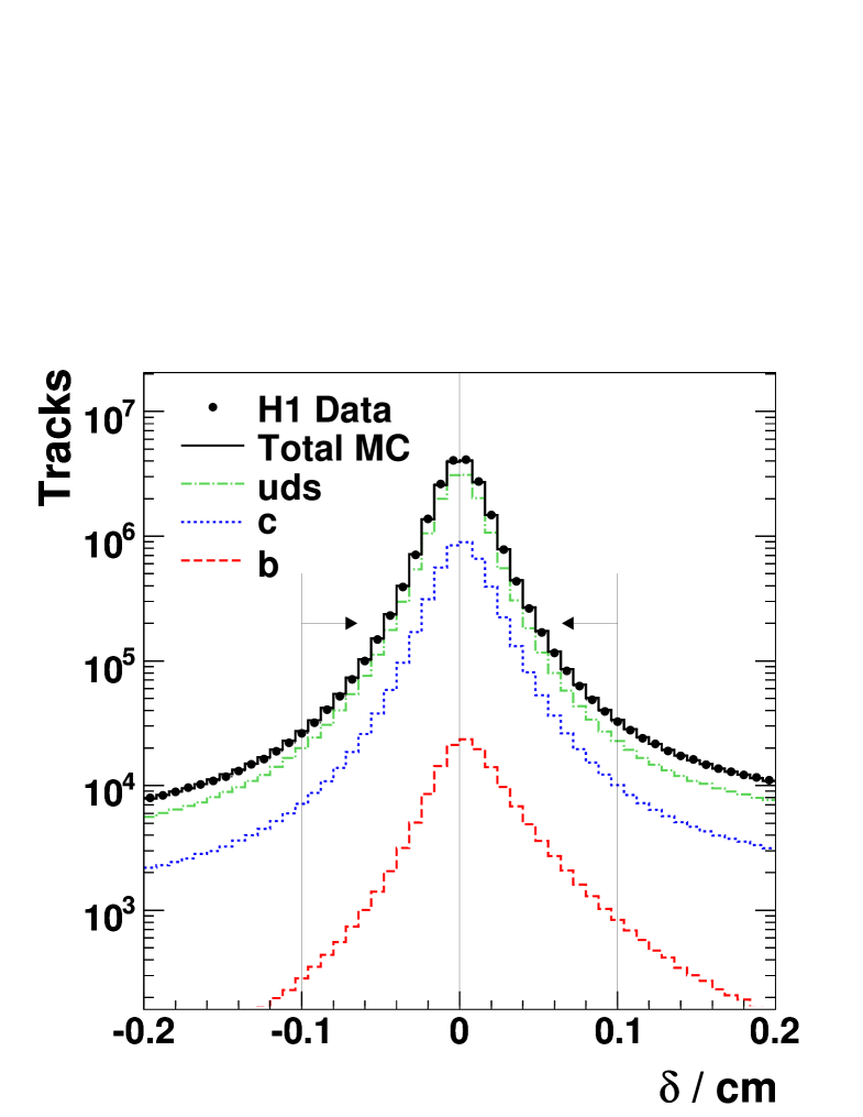
If the angle $\alpha$ between $\phi^{q}$ and the line joining the primary vertex to the point of DCA is less than $90^{\circ}$, $\delta$ is defined as positive. It is defined as negative otherwise. Figure 1 shows an example of a track with positive $\delta$ and one with negative $\delta$. The $\delta$ distribution, shown in figure 2, is seen to be asymmetric with positive values in excess of negative values indicating the presence of long-lived particles. It is found to be well described by the Monte Carlo simulation. CST tracks with $|\delta|>0.1~{}{\rm cm}$ are rejected to suppress light quark events containing long-lived strange particles.

The number of reconstructed CST tracks $N_{\rm track}$ associated to the struck quark is an important quantity since for higher track multiplicities more information can be used. In the kinematic range of this measurement $22\%$ of the events have no selected track, $26\%$ of the events have $N_{\rm track}=1$, $23\%$ have $N_{\rm track}=2$ and $29\%$ have $N_{\rm track}\geq 3$.

4.3 Secondary Vertex Reconstruction

The complete set of reconstructed tracks in the event is used to simultaneously reconstruct a secondary and primary vertex in the transverse plane. Two vertices are reconstructed in each event even if they are not statistically separable. Each track is assigned a weight for each vertex, which is a measure of the probability that the track originated at that vertex[30]. In this approach tracks are not assigned unambiguously to one vertex or the other. A simultaneous fit to the primary and secondary vertex is made, with the weights of all tracks of the event considered for the primary vertex, but only the weights of CST tracks considered for the secondary vertex. The beam spot together with its spread is used as an additional constraint to the primary vertex. The vertex configuration that minimises the global $\chi^{2}$ is found iteratively using deterministic annealing[31].

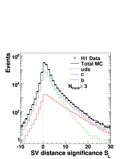
The transverse distance between the secondary and primary vertex is defined as $L_{xy}$. The secondary vertex significance $S_{L}$ is $L_{xy}/\sigma(L_{xy})$, where $\sigma(L_{xy})$ is the uncertainty on $L_{xy}$. If the absolute difference between the azimuthal angle of the secondary vertex (taking the primary vertex as the origin) and $\phi^{q}$ is less than $90^{\circ}$, $S_{L}$ is signed positive and negative otherwise. A measure of the decay multiplicity $N^{\rm SV}_{\rm track}$ is made by counting the number of tracks with weight greater than $0.8$ to the secondary vertex. This method was shown in [9] to yield consistent results with the default method that used track significances.

4.4 Quark Flavour Separation

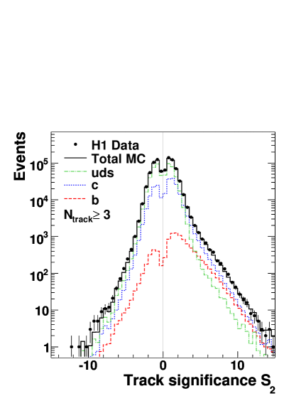
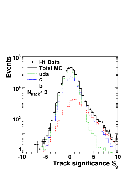
The track significance is defined as $\delta/\sigma(\delta)$, where $\sigma(\delta)$ is the uncertainty on $\delta$. The significances $S_{1}$, $S_{2}$ and $S_{3}$, are defined as the significance of the CST track with the highest, second highest and third highest absolute significance, respectively. The significances take the sign of $\delta$ (see section 4.2). Tracks with a negative sign for significance are likely not to arise from particles with a large lifetime and are used in this analysis to estimate the light quark contribution.

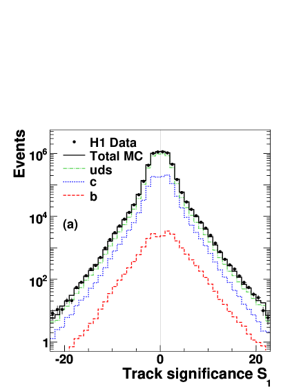
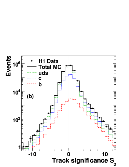
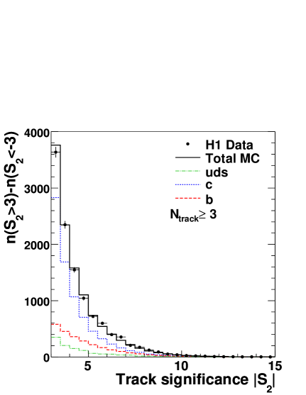
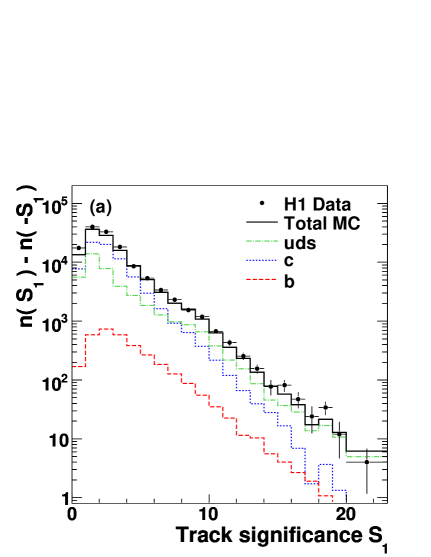
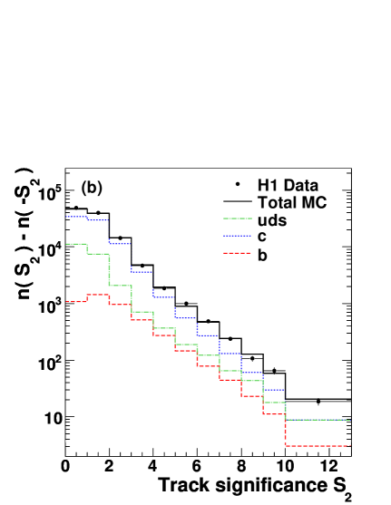
Tracks that do not have the same significance sign as $S_{1}$ are ignored. The $S_{1}$ distribution is used for events with one remaining CST track after this selection and the $S_{2}$ distribution is used if there are two remaining CST tracks. For events with three or more remaining CST tracks, where more information is available, information is combined from the significance distributions and the reconstructed secondary vertex using an artificial neural network (NN) that takes into account correlations of the input variables [32]. In this way each event with at least $1$ CST track appears in exactly one distribution and the distributions are statistically independent. The $S_{1}$ and $S_{2}$ distributions are shown in figure 3.

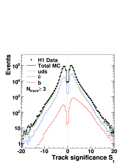
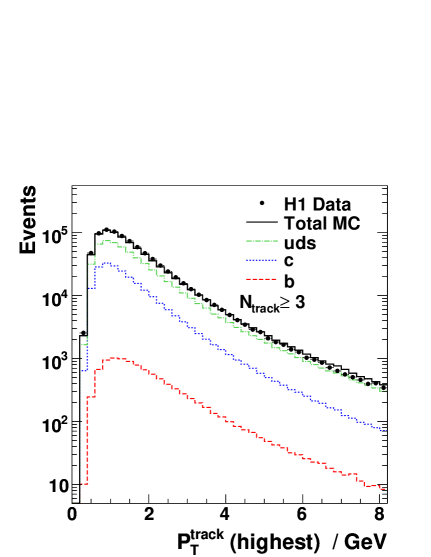
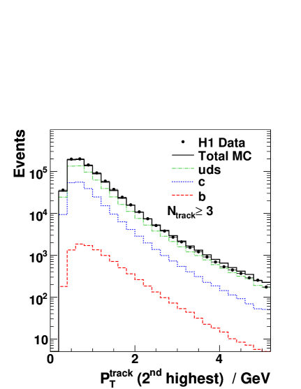
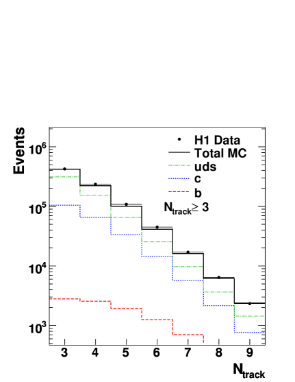
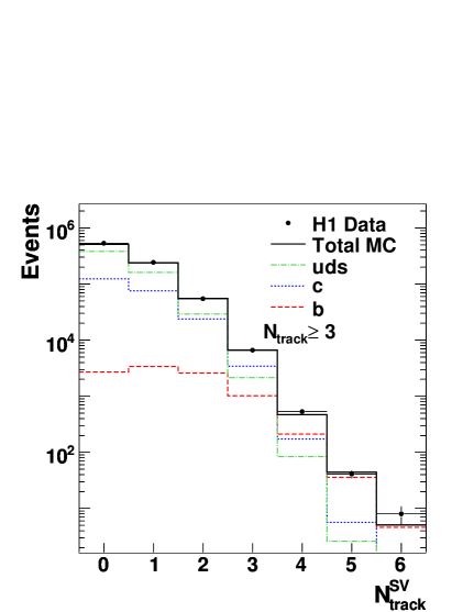
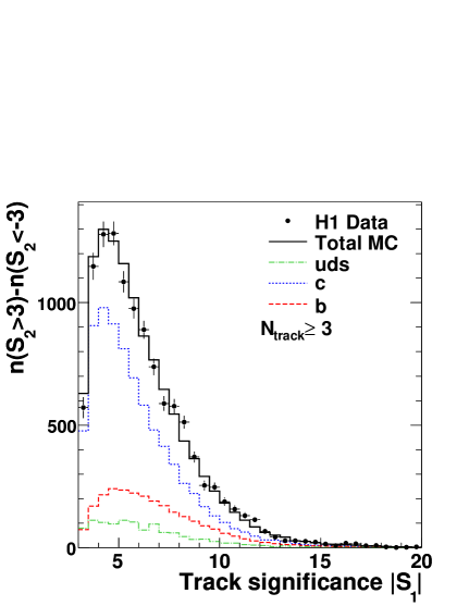
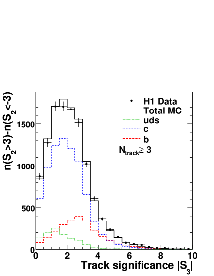
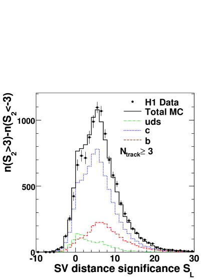
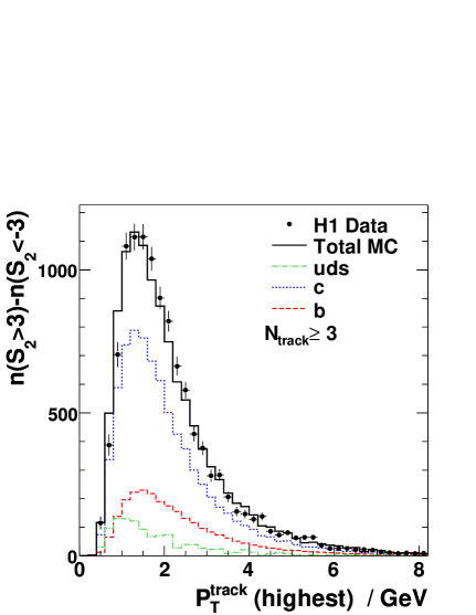
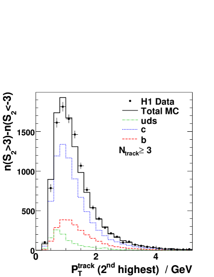
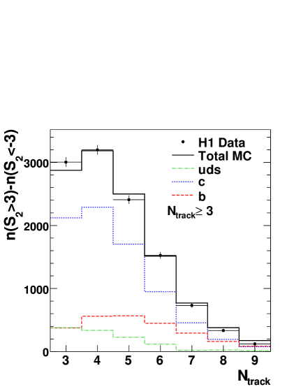
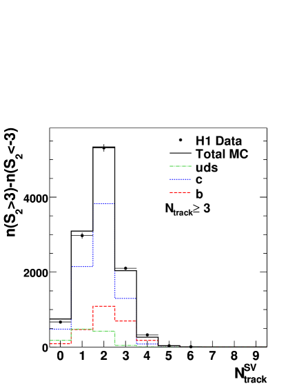
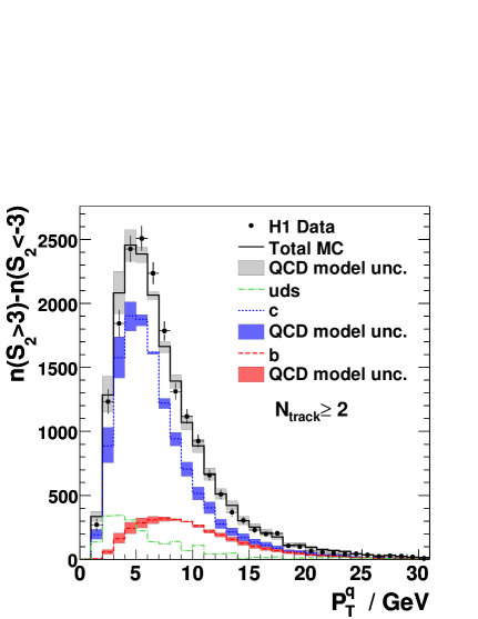
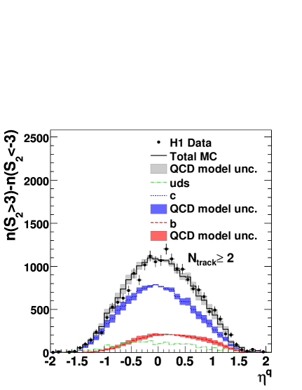
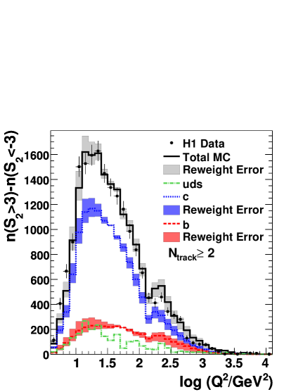
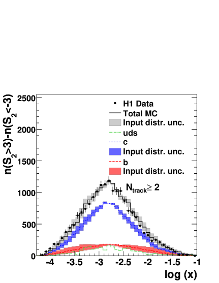
The NN has inputs of $S_{1}$, $S_{2}$, $S_{3}$, $S_{L}$, $N_{\rm track}$, $N^{\rm SV}_{\rm track}$ and $P_{T}^{\rm track}$ of the CST tracks with the highest and second highest transverse momentum. The NN has one hidden layer with $5$ nodes. It was trained using a sample of around $5000$ Monte Carlo $b$ events as ‘signal’ and a similar number of Monte Carlo $c$ events as ‘background’. No attempt is made to discriminate against the light quark events since their impact is minimized by the subtraction procedure described below. The same NN is used for all $y$–$Q^{2}$ bins. The distributions of the NN inputs are shown in figures 4 and 5. These distributions are dominated by light quark events. It can be seen that the Monte Carlo simulation gives a reasonable description of these distributions. It is also apparent that these distributions have good separation power between light, $c$ and $b$ events. The decrease in events around zero for the $S_{1}$ and $S_{2}$ distributions is due to the requirement that $|S_{1}|>|S_{2}|>|S_{3}|$. In order to see how well the Monte Carlo simulation describes the heavy flavour contribution of the NN input distributions, the distribution for those events with $S_{2}>3$ is taken and the distribution for those events with $S_{2}<-3$ is subtracted from it. This has the effect of greatly reducing the light quark distribution which is almost symmetric in $S_{2}$. This subtraction method can be used for any distribution. The subtracted distributions of the NN inputs are shown in figures 6 and 7. The Monte Carlo simulation gives a good description of these distributions. It can be seen that $b$ events tend to have a higher track multiplicity and more tracks at higher $P_{T}$. Other distributions are checked in a similar way. Distributions of variables related to the struck quark, $P_{T}^{q}$ and $\eta^{q}$, as well as the kinematic variables $\log Q^{2}$ and $\log x$ are shown in figure 8 for $N_{\rm track}\geq 2$. The Monte Carlo simulation gives a good description of these distributions.

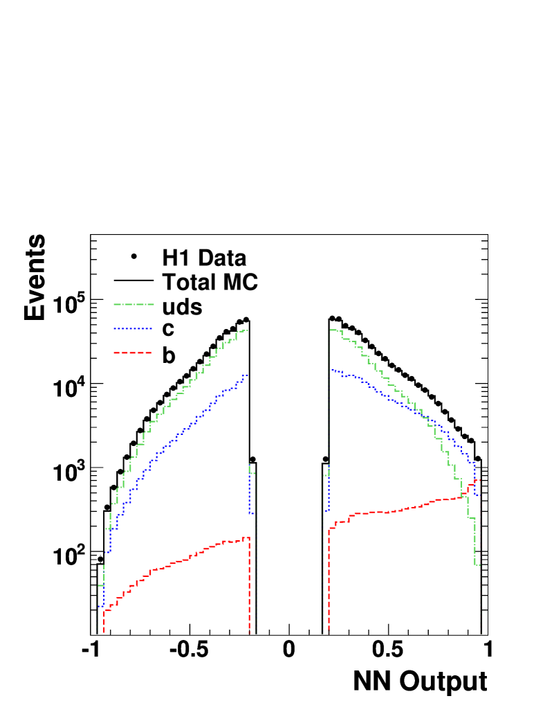
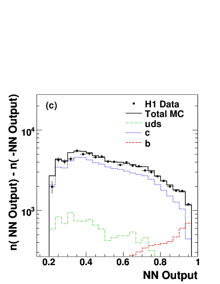
The output of the NN is shown in figure 9. It gives output values in the range from about $0.2$ to $0.95$. The NN output is signed according to the sign of $S_{1}$. It can be seen that: the light quark distribution is approximately symmetric and peaks towards low absolute values; the $c$ and $b$ distributions are asymmetric with more positive than negative entries; the $b$ events are peaked towards $1$, whereas the $c$ events are peaked towards $0$. The Monte Carlo simulation gives a good description of the distribution.

Since the light quark $S_{1}$, $S_{2}$ and NN distributions are nearly symmetric around zero the sensitivity to the modelling of the light quarks can be reduced by subtracting the contents of the negative bins from the contents of the corresponding positive bins. The subtracted distributions are shown in figure 10. The resulting distributions are dominated by $c$ quark events, with a $b$ quark fraction increasing towards the upper end of the distributions. The light quarks contribute a small fraction, although this fraction is larger than in [10], mainly due to the lower $Q^{2}$ and $P_{T}^{\rm track}$ selections in the present analysis.

The fractions of $c$, $b$ and light quarks of the data are extracted in each $y$–$Q^{2}$ interval using a least squares simultaneous fit to the subtracted $S_{1}$, $S_{2}$ and NN distributions (as in figure 10) and the total number of inclusive events before any CST track selection. Only those bins in the significance distributions which have at least $25$ events before subtraction are considered in the fit, since Gaussian errors are assumed. The last fitted bin of the significance distributions, which usually has the lowest statistics, is made $3$ times as wide as the other bins (see figure 10). If any of the bins before subtraction within the NN output range contain less than $25$ events the bin size is doubled, which ensures all bins contain at least $25$ events.

The light, $c$ and $b$ Monte Carlo simulation samples are used as templates. The Monte Carlo light, $c$ and $b$ contributions in each $y$–$Q^{2}$ interval are scaled by factors $\rho_{l}$, $\rho_{c}$ and $\rho_{b}$, respectively, to give the best fit to the observed subtracted $S_{1}$, $S_{2}$ and NN distributions and the total number of inclusive events in each $y-Q^{2}$ interval. Only the statistical errors of the data and Monte Carlo simulation are considered in the fit. The fit to the subtracted significance and NN distributions mainly constrains $\rho_{c}$ and $\rho_{b}$, whereas the overall normalisation constrains $\rho_{l}$.

Since the error on $\rho_{c}$ is much smaller than that of $\rho_{b}$ the $c$ cross section is measured in more $y$–$Q^{2}$ intervals than the $b$ cross section. Therefore two sets of fits are performed, one with a fine binning of $29$ bins and the other with a coarse binning of $12$ bins. The two sets of fits are performed in an identical manner. The results of the two sets of fits are listed in tables 1 and 2. Also included in the tables are the $\chi^{2}/$n.d.f. evaluated using statistical errors only. Acceptable values are obtained for all bins. The fit is also performed to the complete data sample and shown in figure 10. The stability of the method is checked by repeating the fit to the complete data in a variety of ways: fitting the $e^{+}p$ and $e^{-}p$ data separately; using $S_{3}$ instead of the NN; using $S_{L}$ instead of the NN; using the NN alone without $S_{1}$ and $S_{2}$; using $S_{1}$ and $S_{2}$ without the NN; using the NN alone without negative subtraction. All give consistent results within statistical and systematic errors.

The results of the fit in each $y$–$Q^{2}$ interval are converted to a measurement of the ‘reduced $c$ cross section’ defined from the differential cross section as

$$\tilde{\sigma}^{c\bar{c}}(x,Q^{2})=\frac{{\rm d}^{2}\sigma^{c\bar{c}}}{{\rm d}x\,{\rm d}Q^{2}}\frac{xQ^{4}}{2\pi\alpha^{2}(1+(1-y)^{2})},$$ (1)

using:

$$\tilde{\sigma}^{c\bar{c}}(x,Q^{2})=\tilde{\sigma}(x,Q^{2})\frac{\rho_{c}N^{\rm MCgen}_{c}}{\rho_{l}N^{\rm MCgen}_{l}+\rho_{c}N^{\rm MCgen}_{c}+\rho_{b}N^{\rm MCgen}_{b}}\delta_{\rm BCC},$$ (2)

where $\alpha$ is the fine structure constant evaluated with scale $Q^{2}$, and $N^{\rm MCgen}_{l}$, $N^{\rm MCgen}_{c}$, and $N^{\rm MCgen}_{b}$ are the number of light, $c$, and $b$ quark events generated from the Monte Carlo simulation in each bin. The inclusive reduced cross section $\tilde{\sigma}(x,Q^{2})$ is taken from H1 measurements: Tables 17 and 19 from [33], Tables 10 and 11 from [34] and Table 11 from [35]. A bin centre correction $\delta_{\rm BCC}$ is applied using a NLO QCD expectation for $\tilde{\sigma}^{c\bar{c}}$ and $\tilde{\sigma}$ to convert the bin averaged measurement into a measurement at a given $x$–$Q^{2}$ point. This NLO QCD expectation is calculated from the results of a fit similar to that performed in [36] but using the massive scheme to generate heavy flavours.

The reduced cross section is corrected using the Monte Carlo simulation for pure QED radiative effects. The photoproduction background is not subtracted, which, due to the method used to calculate the reduced cross sections, means that the fraction of $c$ and $b$ events in the photoproduction background is assumed to be the same as in the DIS data. In most of the $y$ range the background from photoproduction events is negligible and does not exceed $4\%$ in any $y$–$Q^{2}$ interval used in this analysis. Events that contain $c$ hadrons via the decay of $b$ hadrons are not included in the definition of the reduced $c$ cross section. The reduced $b$ cross section is evaluated in the same manner.

5 Systematic Uncertainties

The following uncertainties are taken into account in order to evaluate the systematic error.

• An uncertainty in the $\delta$ resolution of the tracks is estimated by varying the resolution by an amount that encompasses any difference between the data and simulation evaluated from figure 2. This was achieved by applying an additional Gaussian smearing in the Monte Carlo simulation of $200$ $\mu{\rm m}$ to $5\%$ of randomly selected tracks and $12$ $\mu{\rm m}$ to the rest.

• A track efficiency uncertainty is assigned of $1\%$ due to the CTD and of $2\%$ due to the CST.

• The uncertainties on the various $D$ and $B$ meson lifetimes, decay branching fractions and mean charge multiplicities are estimated by varying the input values of the Monte Carlo simulation by the errors on the world average measurements. For the branching fractions of $b$ quarks to hadrons and the lifetimes of the $D$ and $B$ mesons the central values and errors on the world averages are taken from[37]. For the branching fractions of $c$ quarks to hadrons the values and uncertainties are taken from[38], which are consistent with measurements made in DIS at HERA[39]. For the mean charged track multiplicities the values and uncertainties for $c$ and $b$ quarks are taken from MarkIII[40] and LEP/SLD[41] measurements, respectively.

• The uncertainty on the fragmentation function of the heavy quarks is estimated by reweighting the events according to the longitudinal string momentum fraction $z$ carried by the heavy hadron in the Lund model using weights of $(1\mp 0.7)\cdot(1-z)+z\cdot(1\pm 0.7)$ for charm quarks and of $(1\mp 0.5)\cdot(1-z)+z\cdot(1\pm 0.5)$ for beauty quarks. The variations for the charm fragmentation are motivated by comparison of the Monte Carlo simulation with H1 data [42].

• An uncertainty on the QCD model of heavy quark production is estimated by reweighting the jet transverse momentum and pseudorapidity by $(P^{\rm jet}_{T}/(10~{}{\rm GeV}))^{\pm 0.2}$ and $(1\pm\eta^{\rm jet})^{\pm 0.15}$ for charm jets and $(P^{\rm jet}_{T}/(10~{}{\rm GeV}))^{\pm 0.3}$ and $(1\pm\eta^{\rm jet})^{\pm 0.3}$ for bottom jets. These values are obtained by comparing these variations with the measured reduced cross section for $b$ and $c$ jets[43]. The effects of each of these uncertainties on the subtracted reconstructed distributions of $P_{T}^{q}$ and $\eta_{q}$ are shown in figure 8, where the data is seen to be consistent with the Monte Carlo simulation within the uncertainties.

• The uncertainty on the asymmetry of the light quark $\delta$ distribution is estimated by repeating the fits with the subtracted light quark distributions (figure 10) changed by $\pm 30\%$. The light quark asymmetry was checked to be within this uncertainty by comparing the asymmetry of Monte Carlo simulation events to that of the data for $K^{0}$ candidates, in the region $0.1<|\delta|<0.5~{}{\rm cm}$, where the light quark asymmetry is enhanced.

• An error on $\phi^{q}$ is estimated by shifting $\phi^{q}$ by $2^{\circ}$($5^{\circ}$) for events with (without) a reconstructed jet. These shifts were estimated by comparing the difference between $\phi^{q}$ and the track azimuthal angle in data and Monte Carlo simulation.

• The uncertainty on the hadronic energy scale is estimated by changing the hadronic energy by $\pm 2\%$.

• The uncertainty in the photoproduction background is taken as $100\%$ of the fraction of photoproduction events in each bin, for events with $N_{\rm track}\geq 1$.

• Uncertainties on the acceptance and bin centre correction due to the input heavy quark structure functions used are estimated by reweighting the input $\tilde{\sigma}^{c\bar{c}}$ distribution by $x^{\pm 0.1}$ and $1\pm 0.2\ln[Q^{2}/(10~{}{\rm GeV}^{2})]$ and $\tilde{\sigma}^{b\bar{b}}$ by $x^{\pm 0.3}$ and $1\pm 0.4\ln[Q^{2}/(10~{}{\rm GeV}^{2})]$. The range of variation of the input structure functions was estimated by comparing to the measured values obtained in this analysis. The effects of each of these uncertainties on the subtracted distributions of $\log Q^{2}$ and $\log x$ are shown in figure 8, where the data is seen to be consistent with the Monte Carlo simulation within the uncertainties.

The above systematic uncertainties are evaluated by making the changes described above to the Monte Carlo simulation and repeating the procedure to evaluate the reduced $c$ and $b$ cross sections, including the fits. The uncertainties are evaluated separately for each $x$–$Q^{2}$ measurement.

Additional contributions to the systematic error due to the inclusive cross section are taken from the corresponding $x$–$Q^{2}$ bin in [33, 34, 35], since the measurements are normalised to the inclusive cross section measurements (see equation 2). The error due to the inclusive DIS selection includes a $1.1$–$1.5\%$ uncertainty on the luminosity measurement; an uncertainty on the scattered electron polar angle of $0.2$–$3.0~{}{\rm mrad}$ and energy of $0.2$–$2.0\%$ depending on the energy and angle; typically $<1\%$ combined error due to trigger and scattered electron identification efficiency; and a $0.5$–$1.0\%$ uncertainty on the reduced cross section evaluation due to QED radiative corrections.

A detailed list of the systematic effect on each reduced cross section measurement is given in tables 3 and 4. The errors of $\delta$ resolution and track efficiency are considered uncorrelated between the HERA I and HERA II datasets. All other errors are assumed $100\%$ correlated.

6 Results

6.1 Comparison and Combination of Data

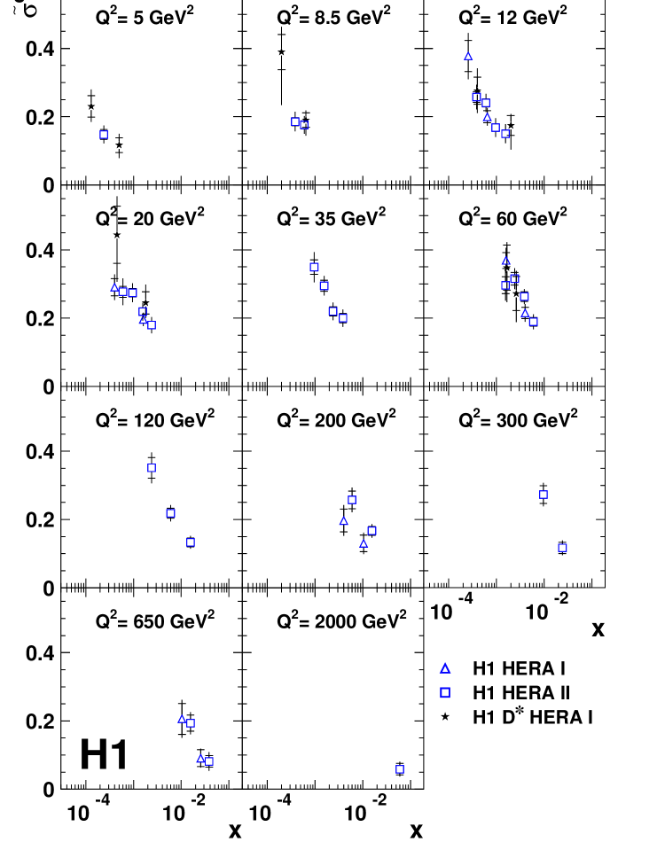
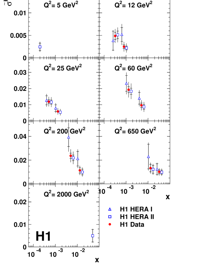
The measurements of $\tilde{\sigma}^{c\bar{c}}$ and $\tilde{\sigma}^{b\bar{b}}$ are shown as a function of $x$ for fixed values of $Q^{2}$ in figures 11 and 12 respectively. Also shown in these figures are the HERA I data extracted using measurements based on the displacement of tracks[9, 10]. The HERA I measurements for $Q^{2}\leq 60\ {\rm GeV^{2}}$ are normalised to the H1 inclusive cross sections measurements from [33] and [34]. The $\tilde{\sigma}^{c\bar{c}}$ and $\tilde{\sigma}^{b\bar{b}}$ data from HERA I and HERA II show good agreement for all measured $x$ and $Q^{2}$ values. In figure 11 the $\tilde{\sigma}^{c\bar{c}}$ data are also compared with those extracted from $D^{*}$ meson measurements by H1 [12], which were obtained using a NLO program [44] based on DGLAP evolution to extrapolate the measurements outside the visible $D^{*}$ range. The $D^{*}$ data agree well with the measurements from the present analysis.

The HERA I and HERA II datasets are combined for each $x$-$Q^{2}$ point where there are two measurements. The combination is performed using a weighted mean using those errors considered uncorrelated between the two data sets (the statistical errors and the systematic errors of $\delta$ resolution and track efficiency, see section 5):

$$\sigma_{\rm comb}=w_{I}\sigma_{\rm I}+w_{II}\sigma_{\rm II},$$ (3)

$${\rm with}\,\,\,\,w_{I}=\frac{\delta^{2}_{\rm II}}{\delta^{2}_{\rm I}+\delta^{2}_{\rm II}}\,\,\,\,{\rm and}\,\,\,\,w_{II}=\frac{\delta^{2}_{\rm I}}{\delta^{2}_{\rm I}+\delta^{2}_{\rm II}},$$ (4)

where $\sigma_{\rm comb}$ is the combined measurement and $\sigma_{\rm I}$ and $\sigma_{\rm II}$ are the HERA I and HERA II measurements respectively, with their respective errors of $\delta_{\rm I}=\sum_{i}\delta^{i}_{\rm I}$ and $\delta_{\rm II}=\sum_{i}\delta^{i}_{\rm II}$, where $i$ denotes the statistical error and each source of uncorrelated error between the two data sets. These contributions to the combined error are evaluated as:

$$(\delta^{i}_{\rm comb})^{2}=(w_{I}\delta^{i}_{\rm I})^{2}+(w_{II}\delta^{i}_{\rm II})^{2}.$$ (5)

For those systematics $j$ considered correlated between the two datasets (all apart from the errors of $\delta$ resolution and track efficiency) the systematic error as evaluated from HERA II is taken, $\delta^{j}_{\rm II}$. The total error on the combined measurement is therefore evaluated from:

$$(\delta^{\rm tot}_{\rm comb})^{2}=\sum_{i}(\delta^{i}_{\rm comb})^{2}+\sum_{j}(\delta^{j}_{\rm II})^{2}.$$ (6)

All data that is subsequently shown is from the combined dataset. Tables 3 and 4 list the combined results for $c$ and $b$. The results listed in these tables supersede the HERA I measurements published in [9] and [10]. If fits are performed with the data listed in these tables it should be noted that, although each $x$–$Q^{2}$ measurement is statistically independent, there is a correlation between the $c$ and $b$ measurements. Since the $c$ and $b$ binning is very different this correlation may be neglected for most bins. However, for the first and last bin the binning is identical so the correlation coefficient $C_{bc}$ listed in table 1 should be used.

6.2 Comparison with QCD

The leading contribution to heavy flavour production in the region $Q^{2}\raisebox{-3.01385pt}{$\stackrel{{\scriptstyle\textstyle<}}{{\sim}}$}M^{2}$ is given by the massive boson-gluon fusion matrix element [15, 45] convoluted with the gluon density of the proton. In the region where $Q^{2}$ is much larger than $M^{2}$ the massive approach may be a poor approximation due to the large logarithms $\log Q^{2}/M^{2}$ which are not resummed [2]. Here, the heavy quarks can be treated as massless partons with the leading order contribution coming from the quark parton model and the heavy quark parton densities. In QCD fits to global hard-scattering data the parton density functions are usually extracted using the general mass variable flavour number scheme (GM VFNS) [1, 2, 3, 4] for heavy quarks which interpolates from the massive approach at low scales to the massless approach at high scales.

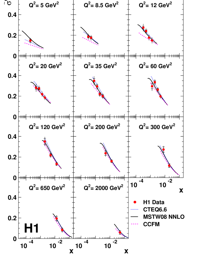
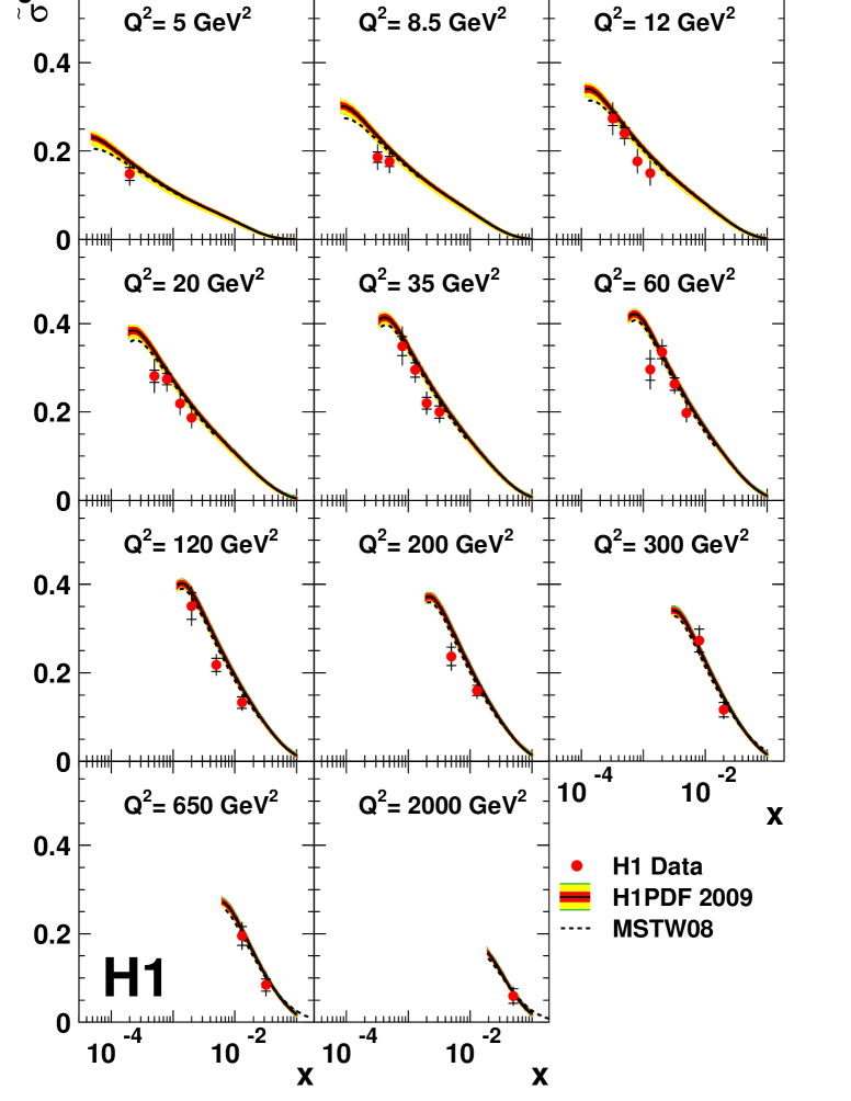
The data are compared with recent QCD predictions based on the GM VFNS from MSTW[7] (at NLO and NNLO), CTEQ[6] (at NLO) and from H1[34] (at NLO). The MSTW predictions use the MSTW08 PDFs which have $m_{c}=1.4~{}{\rm GeV}$ and $m_{b}=4.75~{}{\rm GeV}$, and the renormalization and factorization scales are set to $\mu_{r}=\mu_{f}=Q$. The CTEQ predictions use the CTEQ6.6 PDFs where $m_{c}=1.3~{}{\rm GeV}$, $m_{b}=4.5~{}{\rm GeV}$ and $\mu_{r}=\mu_{f}=\sqrt{Q^{2}+M^{2}}$. The predictions from H1 use the H1PDF 2009 PDFs and the same heavy flavour treatment, including the quark masses and perturbative scales, as for the MSTW08 NLO predictions [7].

The data are also compared with predictions based on CCFM[46] parton evolution and massive heavy flavour production. The CCFM predictions use the A0 PDF set [47] with $m_{c}=1.4~{}{\rm GeV}$, $m_{b}=4.75~{}{\rm GeV}$ and $\mu_{r}=\mu_{f}=\sqrt{\hat{s}+Q_{T}^{2}}$, where $\hat{s}$ is the square of the partonic centre of mass energy and $Q_{T}$ is the transverse momentum of the heavy quark pair.

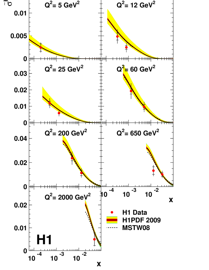
The $\tilde{\sigma}^{c\bar{c}}$ data as a function of $x$ for fixed values of $Q^{2}$ are compared in figure 13 with the QCD predictions from CCFM, CTEQ and MSTW at NNLO, and in figure 14 with the predictions from H1 and MSTW at NLO. In figure 13 the GM VFNS predictions from CTEQ and MSTW at NNLO are observed to be similar with the size of the largest differences between the two being at the level of the total experimental errors on the data. The CTEQ and MSTW predictions provide a reasonable description of the rise of the data with decreasing $x$ across the whole of the measured kinematic range thus supporting the validity of PDFs extracted using the GM VFNS. The predictions based on CCFM evolution tend to undershoot the data at the lowest values of $Q^{2}$ and $x$ but also provide a reasonable description for the rest of the measured phase space. In figure 14 the GM VFNS predictions from H1 and MSTW at NLO, which implement the same heavy flavour treatment [7], are similar and also provide a reasonable description of the data. The H1 predictions are shown with uncertainty bands representing the experimental and theoretical uncertainties [34]. The inner error band describes the experimental fit uncertainty, the middle error band represents the experimental and model uncertainties added in quadrature and the outer error band represents the fit parameterisation uncertainty added in quadrature with all the other uncertainties. The largest contribution to the uncertainty comes from the model which is dominated by the variation of the charm quark mass, which is varied from $1.38$ to $1.47\ {\rm GeV}$. The total uncertainties on the H1PDF 2009 reduced charm cross section predictions are generally smaller than those on the data.

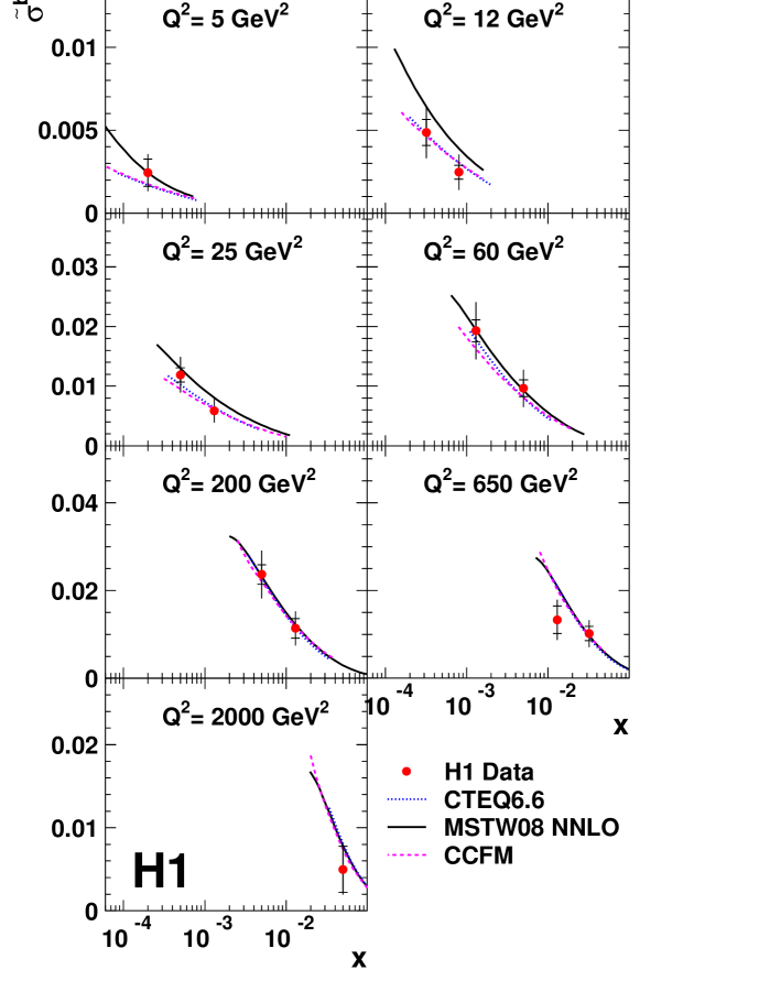
The $\tilde{\sigma}^{b\bar{b}}$ data as a function of $x$ for fixed values of $Q^{2}$ are compared with the QCD predictions in figures 15 and 16. In figure 15 the CTEQ and CCFM predictions are seen to be very similar across the whole range of the measurements. The MSTW NNLO predictions are around $35\%$ higher than CTEQ and CCFM at low values of $Q^{2}$, with the difference decreasing with increasing values of $Q^{2}$. The differences between the theory predictions for the $b$ cross section at low $Q^{2}$ are much reduced compared with the theoretical status at the time of the HERA I publication where there was a factor $2$ difference at $Q^{2}=12\ {\rm GeV^{2}}$ [10]. In figure 16 the MSTW and H1 NLO QCD predictions for $\tilde{\sigma}^{b\bar{b}}$ are observed, as for the case of $\tilde{\sigma}^{c\bar{c}}$, to be very similar. The uncertainty on the H1 predictions is again dominated by the model uncertainty due to the variation of the $b$ quark mass, which is varied from $4.3$ to $5.0\ {\rm GeV}$. At lower values of $Q^{2}$ the uncertainties on the H1 PDF predictions are larger than those on the data. The reduced $b$ cross section data, including the points in the newly measured regions, are well described by all the present QCD predictions.

The structure function $F_{2}^{c\bar{c}}$ is evaluated from the reduced cross section

$$\tilde{\sigma}^{c\bar{c}}=F_{2}^{c\bar{c}}-\frac{y^{2}}{1+(1-y)^{2}}F_{L}^{c\bar{c}},$$ (7)

where the longitudinal structure function $F_{L}^{c\bar{c}}$ is estimated from the same NLO QCD expectation as used for the bin centre correction. The correction due to $F_{L}^{c\bar{c}}$ is negligible for most bins but contributes up to $6.7$% of the reduced cross section at the highest value of $y$. The structure function $F_{2}^{b\bar{b}}$ is evaluated in the same manner.

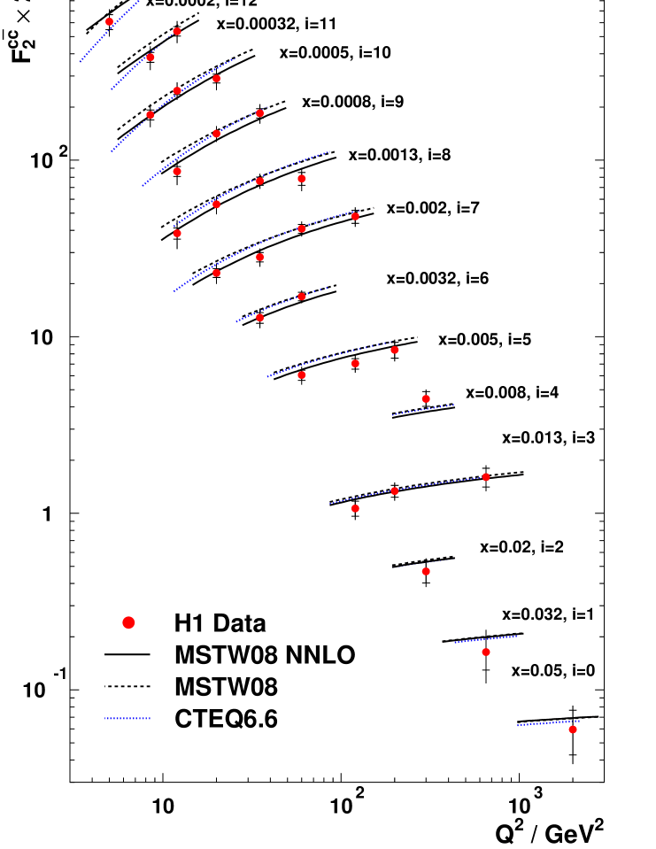
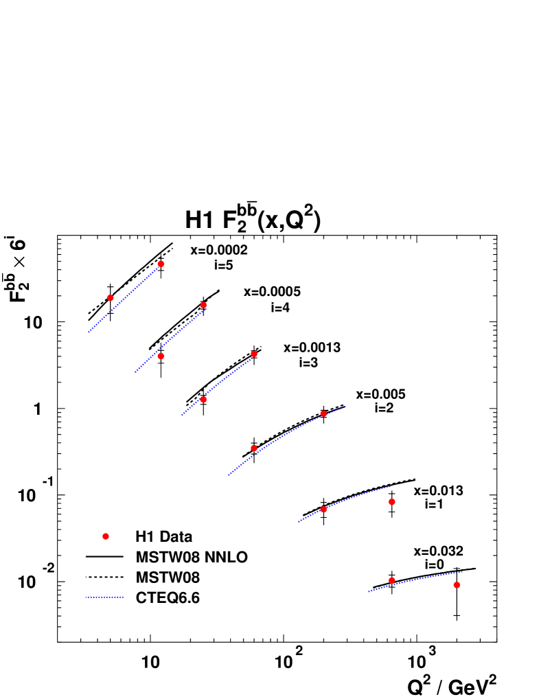
The measurements of $F_{2}^{c\bar{c}}$ and $F_{2}^{b\bar{b}}$ are presented in table 3 and shown as a function of $Q^{2}$ in figure 17 and figure 18 respectively. The data are compared with the GM VFNS QCD predictions from CTEQ[6] at NLO and from MSTW at NLO and NNLO[7]. The description of the charm data by the MSTW QCD calculations is reasonable, with the NNLO being somewhat better than NLO. The CTEQ NLO prediction also gives a reasonable description of the data.

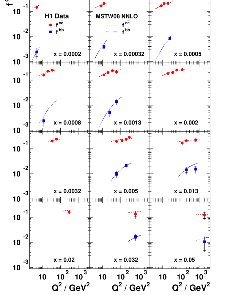
The measurements are presented in figure 19 in the form of the fractional contribution to the total $ep$ cross section

$$f^{c\bar{c}}=\frac{{\rm d}^{2}\sigma^{c\bar{c}}}{{\rm d}x\,{\rm d}Q^{2}}/\frac{{\rm d}^{2}\sigma}{{\rm d}x\,{\rm d}Q^{2}}.$$ (8)

The $b$ fraction $f^{b\bar{b}}$ is defined in the same manner. In the present kinematic range the value of $f^{c\bar{c}}$ is around $17\%$ on average and increases slightly with increasing $Q^{2}$ and decreasing $x$. The value of $f^{b\bar{b}}$ increases rapidly with $Q^{2}$ from about $0.2\%$ at $Q^{2}=5\ {\rm GeV^{2}}$ to around $1\%$ for $Q^{2}\raisebox{-3.01385pt}{$\stackrel{{\scriptstyle\textstyle>}}{{\sim}}$}60\ {\rm GeV^{2}}$. The NNLO QCD predictions of MSTW shown in figure 19 are found to describe the data well.

7 Conclusion

The reduced charm and beauty cross sections in deep inelastic scattering are measured for a wide range of $Q^{2}$ and Bjorken $x$ using the HERA II data. The analysis was performed using several variables including the significance (the impact parameter divided by its error) and the position of the secondary vertex as reconstructed from the vertex detector. For selected track multiplicities of $1$ or $2$ the highest and second highest significance distributions are used to evaluate the charm and beauty content of the data. For selected track multiplicities $\geq 3$ several variables are combined using an artificial neural network.

The reduced cross sections agree with previous measurements using a similar technique, but have reduced errors and cover an extended $Q^{2}$ range. HERA I and HERA II data are combined resulting in more precise reduced cross section and structure function measurements. The charm and beauty fractional contributions to the total $ep$ cross section are also measured. In this kinematic range the charm cross section contributes on average $17\%$ and the beauty fraction increases from about $0.2\%$ at $Q^{2}=5\ {\rm GeV^{2}}$ to $1.0\%$ for $Q^{2}\raisebox{-3.01385pt}{$\stackrel{{\scriptstyle\textstyle>}}{{\sim}}$}60\ {\rm GeV^{2}}$. The measurements are described by predictions using perturbative QCD in the general mass variable flavour number scheme at NLO and NNLO.

bin	$Q^{2}$	$x$	$y$	$\rho_{l}$	$\rho_{c}$	$\rho_{b}$	$\chi^{2}/{\rm n.d.f.}$	$C_{lc}$	$C_{lb}$	$C_{bc}$ [t]
$1$	$5.0$	$0.00020$	$0.246$	$1.27\pm 0.02$	$1.39\pm 0.13$	$1.72\pm 0.58$	$19.9/24$	$-0.99$	$0.56$	$-0.61$
$2$	$8.5$	$0.00050$	$0.167$	$1.15\pm 0.01$	$1.27\pm 0.08$	$0.58\pm 0.56$	$26.4/24$	$-0.99$	$0.57$	$-0.64$
$3$	$8.5$	$0.00032$	$0.262$	$1.15\pm 0.01$	$1.07\pm 0.07$	$0.86\pm 0.22$	$35.9/39$	$-0.99$	$0.52$	$-0.57$
$4$	$12.0$	$0.00130$	$0.091$	$1.11\pm 0.01$	$1.13\pm 0.08$	$0.94\pm 0.92$	$25.6/24$	$-0.98$	$0.62$	$-0.73$
$5$	$12.0$	$0.00080$	$0.148$	$1.14\pm 0.01$	$0.99\pm 0.06$	$1.29\pm 0.41$	$67.3/40$	$-0.98$	$0.59$	$-0.67$
$6$	$12.0$	$0.00050$	$0.236$	$1.09\pm 0.01$	$1.17\pm 0.06$	$0.48\pm 0.24$	$34.9/38$	$-0.99$	$0.52$	$-0.59$
$7$	$12.0$	$0.00032$	$0.369$	$1.15\pm 0.02$	$1.11\pm 0.07$	$0.88\pm 0.21$	$64.3/39$	$-0.99$	$0.55$	$-0.60$
$8$	$20.0$	$0.00200$	$0.098$	$1.12\pm 0.01$	$1.10\pm 0.06$	$1.77\pm 0.72$	$23.3/26$	$-0.97$	$0.62$	$-0.77$
$9$	$20.0$	$0.00130$	$0.151$	$1.14\pm 0.01$	$1.10\pm 0.05$	$0.97\pm 0.30$	$52.3/39$	$-0.98$	$0.57$	$-0.67$
$10$	$20.0$	$0.00080$	$0.246$	$1.15\pm 0.01$	$1.14\pm 0.05$	$0.60\pm 0.21$	$36.5/38$	$-0.98$	$0.52$	$-0.61$
$11$	$20.0$	$0.00050$	$0.394$	$1.25\pm 0.02$	$0.98\pm 0.06$	$1.00\pm 0.15$	$33.2/40$	$-0.99$	$0.56$	$-0.61$
$12$	$35.0$	$0.00320$	$0.108$	$1.12\pm 0.02$	$1.09\pm 0.07$	$0.93\pm 0.72$	$27.2/26$	$-0.96$	$0.62$	$-0.78$
$13$	$35.0$	$0.00200$	$0.172$	$1.18\pm 0.02$	$0.97\pm 0.06$	$1.52\pm 0.35$	$43.5/39$	$-0.97$	$0.58$	$-0.70$
$14$	$35.0$	$0.00130$	$0.265$	$1.19\pm 0.02$	$1.08\pm 0.06$	$0.67\pm 0.22$	$58.2/39$	$-0.98$	$0.54$	$-0.63$
$15$	$35.0$	$0.00080$	$0.431$	$1.25\pm 0.02$	$1.04\pm 0.06$	$1.02\pm 0.17$	$46.5/39$	$-0.99$	$0.57$	$-0.64$
$16$	$60.0$	$0.00500$	$0.118$	$1.15\pm 0.02$	$0.99\pm 0.06$	$2.17\pm 0.49$	$50.6/40$	$-0.95$	$0.59$	$-0.76$
$17$	$60.0$	$0.00320$	$0.185$	$1.16\pm 0.02$	$1.10\pm 0.06$	$0.66\pm 0.25$	$61.6/37$	$-0.96$	$0.52$	$-0.66$
$18$	$60.0$	$0.00200$	$0.295$	$1.15\pm 0.02$	$1.00\pm 0.06$	$0.90\pm 0.20$	$38.6/39$	$-0.97$	$0.52$	$-0.64$
$19$	$60.0$	$0.00130$	$0.454$	$1.32\pm 0.02$	$0.80\pm 0.07$	$1.06\pm 0.18$	$76.8/38$	$-0.98$	$0.57$	$-0.66$
$20$	$120.0$	$0.01300$	$0.091$	$1.13\pm 0.02$	$0.91\pm 0.09$	$1.37\pm 0.46$	$32.4/23$	$-0.95$	$0.61$	$-0.77$
$21$	$120.0$	$0.00500$	$0.236$	$1.20\pm 0.02$	$0.88\pm 0.06$	$1.27\pm 0.20$	$37.0/38$	$-0.96$	$0.55$	$-0.69$
$22$	$120.0$	$0.00200$	$0.591$	$1.25\pm 0.03$	$0.92\pm 0.08$	$0.94\pm 0.17$	$42.5/37$	$-0.97$	$0.54$	$-0.65$
$23$	$200.0$	$0.01300$	$0.151$	$1.14\pm 0.02$	$1.03\pm 0.08$	$0.65\pm 0.21$	$40.7/36$	$-0.95$	$0.53$	$-0.67$
$24$	$200.0$	$0.00500$	$0.394$	$1.19\pm 0.03$	$0.83\pm 0.08$	$0.75\pm 0.16$	$41.1/36$	$-0.97$	$0.53$	$-0.65$
$25$	$300.0$	$0.02000$	$0.148$	$1.08\pm 0.03$	$0.83\pm 0.12$	$1.16\pm 0.27$	$32.7/33$	$-0.95$	$0.52$	$-0.67$
$26$	$300.0$	$0.00800$	$0.369$	$1.12\pm 0.03$	$0.99\pm 0.09$	$0.54\pm 0.17$	$35.8/34$	$-0.96$	$0.51$	$-0.64$
$27$	$650.0$	$0.03200$	$0.200$	$1.08\pm 0.03$	$0.72\pm 0.15$	$0.75\pm 0.29$	$28.2/32$	$-0.96$	$0.52$	$-0.65$
$28$	$650.0$	$0.01300$	$0.492$	$1.09\pm 0.03$	$0.85\pm 0.10$	$0.82\pm 0.16$	$37.0/35$	$-0.96$	$0.54$	$-0.66$
$29$	$2000.0$	$0.05000$	$0.394$	$1.07\pm 0.04$	$0.73\pm 0.20$	$0.67\pm 0.37$	$25.5/25$	$-0.96$	$0.55$	$-0.67$

Table 1: The fit parameters $\rho_{l}$, $\rho_{c}$ and $\rho_{b}$, along with their errors, the $\chi^{2}$ per degree of freedom and the correlation coefficients of the fit parameters for each bin in $Q^{2}$ and $x$. The parameters are shown for the fine binning scheme used to evaluate the reduced $c$ cross section.

bin	$Q^{2}$	$x$	$y$	$\rho_{l}$	$\rho_{c}$	$\rho_{b}$	$\chi^{2}/{\rm n.d.f.}$	$C_{lc}$	$C_{lb}$	$C_{bc}$ [t]
$1$	$5.0$	$0.00020$	$0.246$	$1.27\pm 0.02$	$1.39\pm 0.13$	$1.72\pm 0.58$	$19.9/24$	$-0.99$	$0.56$	$-0.61$
$2$	$12.0$	$0.00032$	$0.369$	$1.17\pm 0.01$	$1.08\pm 0.06$	$1.06\pm 0.17$	$49.4/40$	$-0.99$	$0.55$	$-0.60$
$3$	$12.0$	$0.00080$	$0.148$	$1.12\pm 0.01$	$1.12\pm 0.03$	$0.75\pm 0.15$	$61.0/46$	$-0.99$	$0.54$	$-0.61$
$4$	$25.0$	$0.00050$	$0.492$	$1.29\pm 0.02$	$0.95\pm 0.05$	$1.15\pm 0.13$	$56.3/42$	$-0.99$	$0.57$	$-0.63$
$5$	$25.0$	$0.00130$	$0.189$	$1.15\pm 0.01$	$1.08\pm 0.02$	$0.93\pm 0.13$	$67.3/45$	$-0.98$	$0.55$	$-0.65$
$6$	$60.0$	$0.00130$	$0.454$	$1.20\pm 0.01$	$0.91\pm 0.03$	$1.00\pm 0.10$	$61.1/43$	$-0.97$	$0.54$	$-0.65$
$7$	$60.0$	$0.00500$	$0.118$	$1.13\pm 0.01$	$1.01\pm 0.04$	$1.16\pm 0.20$	$51.3/44$	$-0.96$	$0.55$	$-0.71$
$8$	$200.0$	$0.00500$	$0.394$	$1.14\pm 0.02$	$0.83\pm 0.04$	$0.88\pm 0.09$	$35.6/40$	$-0.97$	$0.55$	$-0.67$
$9$	$200.0$	$0.01300$	$0.151$	$1.19\pm 0.02$	$1.06\pm 0.07$	$1.01\pm 0.24$	$35.3/39$	$-0.95$	$0.53$	$-0.68$
$10$	$650.0$	$0.01300$	$0.492$	$1.07\pm 0.03$	$0.91\pm 0.09$	$0.50\pm 0.13$	$42.9/36$	$-0.97$	$0.55$	$-0.66$
$11$	$650.0$	$0.03200$	$0.200$	$1.08\pm 0.02$	$0.74\pm 0.09$	$1.12\pm 0.19$	$48.8/37$	$-0.96$	$0.52$	$-0.65$
$12$	$2000.0$	$0.05000$	$0.394$	$1.07\pm 0.04$	$0.73\pm 0.20$	$0.67\pm 0.37$	$25.5/25$	$-0.96$	$0.55$	$-0.67$

Table 2: The fit parameters $\rho_{l}$, $\rho_{c}$ and $\rho_{b}$, along with their errors, the $\chi^{2}$ per degree of freedom and the correlation coefficients of the fit parameters for each bin in $Q^{2}$ and $x$. The parameters are shown for the coarse binning scheme used to evaluate the reduced $b$ cross section.

bin	$Q^{2}$	$x$	$y$	$\tilde{\sigma}^{q\bar{q}}$	$F^{q\bar{q}}_{2}$	$\delta_{\rm stat}$	$\delta_{\rm sys}$	$\delta_{\rm tot}$	$\delta_{\rm unc}$	$\delta_{\rm res}$	$\delta_{\rm effCJC}$	$\delta_{\rm effCST}$	$\delta_{\rm fragC}$	$\delta_{\rm fragB}$	$\delta_{uds}$	$\delta_{\phi^{q}}$	$\delta_{\rm hadE}$	$\delta_{\rm gp}$	$\delta_{\rm F_{2}}$     [t]
	(GeV2)					($\%$)	($\%$)	($\%$)	($\%$)	($\%$)	($\%$)	($\%$)	($\%$)	($\%$)	($\%$)	($\%$)	($\%$)	($\%$)	($\%$)
$c$ 1	$5.0$	$0.00020$	$0.246$	$0.148$	$0.149$	$9.8$	$14.6$	$17.6$	$3.3$	$1.9$	$-1.9$	$-2.8$	$-3.5$	$0.3$	$-7.7$	$4.6$	$-1.2$	$3.1$	$1.0$
$c$ 2	$8.5$	$0.00050$	$0.167$	$0.176$	$0.176$	$6.5$	$13.3$	$14.8$	$2.0$	$1.9$	$-1.3$	$-2.0$	$-2.8$	$0.0$	$-10.0$	$1.8$	$-1.2$	$0.4$	$1.0$
$c$ 3	$8.5$	$0.00032$	$0.262$	$0.186$	$0.187$	$6.4$	$14.1$	$15.5$	$3.8$	$1.1$	$-1.0$	$-1.5$	$-5.8$	$0.0$	$-7.2$	$2.1$	$-0.2$	$3.6$	$1.0$
$c$ 4	$12.0$	$0.00130$	$0.091$	$0.150$	$0.150$	$7.3$	$17.2$	$18.7$	$1.2$	$1.5$	$-0.6$	$-0.9$	$-2.5$	$0.1$	$-15.7$	$1.7$	$1.7$	$0.0$	$1.0$
$c$ 5	$12.0$	$0.00080$	$0.148$	$0.177$	$0.177$	$5.2$	$15.0$	$15.9$	$1.3$	$1.0$	$-0.8$	$-1.3$	$-2.5$	$0.0$	$-13.5$	$1.2$	$-0.7$	$0.2$	$1.1$
$c$ 6	$12.0$	$0.00050$	$0.236$	$0.240$	$0.242$	$4.9$	$10.1$	$11.2$	$1.3$	$2.0$	$-1.0$	$-1.4$	$-3.0$	$0.0$	$-5.6$	$1.7$	$-1.7$	$0.6$	$1.0$
$c$ 7	$12.0$	$0.00032$	$0.369$	$0.273$	$0.277$	$5.6$	$12.6$	$13.8$	$1.4$	$2.1$	$-0.8$	$-1.3$	$-5.6$	$0.1$	$-5.8$	$1.6$	$-0.3$	$3.1$	$1.1$
$c$ 8	$20.0$	$0.00200$	$0.098$	$0.187$	$0.188$	$4.0$	$12.0$	$12.7$	$1.6$	$1.4$	$-0.4$	$-0.8$	$-2.2$	$0.2$	$-9.9$	$1.2$	$2.2$	$0.0$	$1.1$
$c$ 9	$20.0$	$0.00130$	$0.151$	$0.219$	$0.219$	$4.6$	$11.0$	$11.9$	$1.2$	$1.2$	$-0.9$	$-1.4$	$-2.2$	$0.0$	$-8.7$	$1.6$	$0.7$	$0.2$	$1.1$
$c$ 10	$20.0$	$0.00080$	$0.246$	$0.274$	$0.276$	$4.5$	$9.2$	$10.2$	$1.2$	$1.5$	$-1.0$	$-1.4$	$-2.6$	$0.0$	$-5.8$	$1.4$	$-0.8$	$0.5$	$1.0$
$c$ 11	$20.0$	$0.00050$	$0.394$	$0.281$	$0.287$	$4.9$	$12.9$	$13.8$	$1.5$	$1.6$	$-0.5$	$-0.7$	$-5.9$	$0.2$	$-6.7$	$1.7$	$-1.3$	$3.2$	$1.1$
$c$ 12	$35.0$	$0.00320$	$0.108$	$0.200$	$0.200$	$6.9$	$10.7$	$12.7$	$1.9$	$2.4$	$-0.6$	$-0.8$	$-1.8$	$0.3$	$-8.8$	$1.2$	$3.0$	$0.1$	$1.1$
$c$ 13	$35.0$	$0.00200$	$0.172$	$0.220$	$0.220$	$6.1$	$10.1$	$11.8$	$1.5$	$1.9$	$-0.7$	$-1.0$	$-1.9$	$0.0$	$-7.9$	$2.5$	$-0.3$	$0.2$	$1.0$
$c$ 14	$35.0$	$0.00130$	$0.265$	$0.295$	$0.297$	$5.4$	$8.1$	$9.7$	$1.2$	$2.2$	$-0.7$	$-1.0$	$-2.0$	$0.0$	$-5.4$	$1.4$	$-0.4$	$0.3$	$1.0$
$c$ 15	$35.0$	$0.00080$	$0.431$	$0.349$	$0.360$	$6.1$	$11.1$	$12.7$	$1.3$	$0.6$	$-0.5$	$-0.8$	$-4.6$	$0.1$	$-6.4$	$2.0$	$-1.0$	$1.8$	$1.1$
$c$ 16	$60.0$	$0.00500$	$0.118$	$0.198$	$0.199$	$5.1$	$9.5$	$10.8$	$1.8$	$1.9$	$-0.5$	$-0.8$	$-1.7$	$0.7$	$-6.8$	$2.3$	$1.2$	$0.1$	$1.1$
$c$ 17	$60.0$	$0.00320$	$0.185$	$0.263$	$0.264$	$5.5$	$6.3$	$8.4$	$1.1$	$1.5$	$-0.7$	$-1.1$	$-1.5$	$0.0$	$-3.3$	$2.6$	$1.3$	$0.0$	$1.0$
$c$ 18	$60.0$	$0.00200$	$0.295$	$0.335$	$0.339$	$4.3$	$7.7$	$8.8$	$1.1$	$1.8$	$-0.5$	$-0.8$	$-1.5$	$0.1$	$-5.8$	$1.7$	$-0.3$	$0.1$	$1.0$
$c$ 19	$60.0$	$0.00130$	$0.454$	$0.296$	$0.307$	$8.3$	$12.6$	$15.1$	$1.2$	$1.6$	$-0.1$	$-0.2$	$-3.7$	$0.2$	$-9.6$	$1.5$	$-1.3$	$1.0$	$1.0$
$c$ 20	$120.0$	$0.01300$	$0.091$	$0.133$	$0.133$	$9.7$	$10.2$	$14.1$	$2.7$	$2.6$	$-0.7$	$-1.0$	$-2.2$	$0.9$	$-7.7$	$3.2$	$1.2$	$0.0$	$1.2$
$c$ 21	$120.0$	$0.00500$	$0.236$	$0.218$	$0.220$	$6.8$	$8.8$	$11.1$	$1.6$	$2.5$	$-0.3$	$-0.5$	$-1.2$	$0.1$	$-6.6$	$3.1$	$0.7$	$0.0$	$1.1$
$c$ 22	$120.0$	$0.00200$	$0.591$	$0.351$	$0.375$	$8.6$	$9.5$	$12.8$	$3.2$	$3.3$	$-0.3$	$-0.4$	$-2.7$	$0.2$	$-5.1$	$1.9$	$0.0$	$0.9$	$2.9$
$c$ 23	$200.0$	$0.01300$	$0.151$	$0.160$	$0.160$	$7.1$	$9.5$	$11.9$	$2.8$	$2.1$	$-1.0$	$-1.5$	$-1.8$	$0.2$	$-6.5$	$3.1$	$1.7$	$0.0$	$2.7$
$c$ 24	$200.0$	$0.00500$	$0.394$	$0.237$	$0.243$	$8.8$	$10.2$	$13.5$	$3.4$	$3.3$	$-0.1$	$-0.2$	$-2.0$	$0.0$	$-6.2$	$3.7$	$0.3$	$0.5$	$2.9$
$c$ 25	$300.0$	$0.02000$	$0.148$	$0.117$	$0.117$	$14.1$	$12.0$	$18.5$	$3.3$	$2.6$	$-0.4$	$-0.6$	$-1.3$	$0.4$	$-9.3$	$3.8$	$1.9$	$0.0$	$2.9$
$c$ 26	$300.0$	$0.00800$	$0.369$	$0.273$	$0.278$	$9.5$	$8.4$	$12.7$	$3.3$	$3.6$	$-0.2$	$-0.3$	$-1.1$	$0.0$	$-3.4$	$4.8$	$-0.1$	$0.5$	$2.9$
$c$ 27	$650.0$	$0.03200$	$0.200$	$0.084$	$0.085$	$16.7$	$26.0$	$30.9$	$3.8$	$5.2$	$-2.2$	$-3.3$	$-3.4$	$0.2$	$-20.8$	$10.7$	$4.5$	$0.0$	$3.4$
$c$ 28	$650.0$	$0.01300$	$0.492$	$0.195$	$0.203$	$10.8$	$12.0$	$16.2$	$3.7$	$3.0$	$-0.1$	$-0.2$	$-1.0$	$0.2$	$-6.9$	$6.9$	$-0.2$	$0.4$	$3.3$
$c$ 29	$2000.0$	$0.05000$	$0.394$	$0.059$	$0.060$	$28.3$	$22.9$	$36.4$	$6.7$	$4.0$	$-1.7$	$-2.6$	$-1.2$	$0.1$	$-14.1$	$15.6$	$0.0$	$0.2$	$4.3$
$b$ 1	$5.0$	$0.00020$	$0.246$	$0.00244$	$0.00244$	$33.8$	$31.3$	$46.1$	$8.1$	$-2.4$	$-2.8$	$-5.6$	$-3.7$	$-6.6$	$6.0$	$-3.7$	$3.1$	$3.1$	$1.0$
$b$ 2	$12.0$	$0.00032$	$0.369$	$0.00487$	$0.00490$	$16.0$	$27.4$	$31.8$	$8.4$	$-3.4$	$-4.1$	$-8.2$	$-1.1$	$-4.5$	$5.1$	$2.2$	$-0.8$	$4.1$	$1.1$
$b$ 3	$12.0$	$0.00080$	$0.148$	$0.00247$	$0.00248$	$16.7$	$40.2$	$43.5$	$9.6$	$-8.1$	$-7.4$	$-14.8$	$-1.6$	$-5.3$	$17.8$	$2.2$	$6.6$	$0.6$	$1.1$
$b$ 4	$25.0$	$0.00050$	$0.492$	$0.01189$	$0.01206$	$10.1$	$23.0$	$25.1$	$5.0$	$-4.0$	$-3.8$	$-7.5$	$0.2$	$-4.5$	$3.5$	$0.8$	$0.3$	$3.1$	$1.3$
$b$ 5	$25.0$	$0.00130$	$0.189$	$0.00586$	$0.00587$	$12.1$	$31.9$	$34.1$	$7.8$	$-8.7$	$-5.6$	$-11.2$	$-0.8$	$-4.9$	$10.5$	$0.9$	$3.5$	$0.2$	$1.0$
$b$ 6	$60.0$	$0.00130$	$0.454$	$0.01928$	$0.01969$	$9.5$	$23.1$	$25.0$	$10.9$	$-4.6$	$-4.0$	$-8.1$	$-0.1$	$-2.9$	$4.1$	$1.4$	$0.7$	$0.8$	$1.0$
$b$ 7	$60.0$	$0.00500$	$0.118$	$0.00964$	$0.00965$	$14.6$	$29.1$	$32.6$	$4.3$	$-7.0$	$-5.2$	$-10.4$	$-0.5$	$-7.9$	$2.3$	$-2.8$	$8.6$	$0.0$	$1.1$
$b$ 8	$200.0$	$0.00500$	$0.394$	$0.02365$	$0.02422$	$9.4$	$21.2$	$23.2$	$7.9$	$-4.6$	$-4.2$	$-8.5$	$0.2$	$-2.7$	$1.1$	$1.0$	$0.5$	$1.9$	$2.9$
$b$ 9	$200.0$	$0.01300$	$0.151$	$0.01139$	$0.01142$	$19.5$	$28.4$	$34.4$	$4.6$	$-4.4$	$-4.5$	$-8.9$	$0.2$	$-10.3$	$5.7$	$0.0$	$10.4$	$0.0$	$2.7$
$b$ 10	$650.0$	$0.01300$	$0.492$	$0.01331$	$0.01394$	$23.6$	$25.4$	$34.7$	$13.4$	$-4.6$	$-5.0$	$-10.1$	$-1.1$	$-2.2$	$5.8$	$4.5$	$1.5$	$0.8$	$3.3$
$b$ 11	$650.0$	$0.03200$	$0.200$	$0.01018$	$0.01024$	$16.0$	$25.5$	$30.1$	$10.8$	$-3.3$	$-3.3$	$-6.5$	$-0.2$	$-9.0$	$3.6$	$2.1$	$3.1$	$0.0$	$3.4$
$b$ 12	$2000.0$	$0.05000$	$0.394$	$0.00499$	$0.00511$	$55.7$	$25.1$	$61.1$	$15.0$	$-2.0$	$-4.4$	$-8.7$	$1.7$	$-2.7$	$9.4$	$-3.0$	$1.7$	$0.2$	$4.3$

Table 3: The measured values and relative errors for the reduced DIS cross section ($\tilde{\sigma}^{q\bar{q}}$) and structure function $F_{2}^{q\bar{q}}$ for charm ($c$) and beauty ($b$) quarks for the combined datasets. The values for $F_{2}^{q\bar{q}}$ are obtained from the measured reduced cross sections using the NLO QCD fit to correct for the contributions from $F_{L}^{q\bar{q}}$. The table shows the statistical error ($\delta_{\rm stat}$), the systematic error ($\delta_{\rm sys}$), the total error ($\delta_{\rm tot}$) and the uncorrelated systematic error ($\delta_{\rm unc}$) on the reduced cross section. The next ten columns show the effect of a $+1\sigma$ shift for the correlated systematic error contributions to the reduced cross section from: track impact parameter resolution, CJC track efficiency, CST track efficiency, $c$ fragmentation, $b$ fragmentation, light quark contribution, struck quark angle $\phi^{q}$, hadronic energy scale, photoproduction background and the DIS event selection. The $-1\sigma$ errors are taken as the negative of the $+1\sigma$ errors. The correlated systematic errors are continued in table 4.

bin	$\delta_{{\rm mod}Q^{2}c}$	$\delta_{{\rm mod}Q^{2}b}$	$\delta_{{\rm mod}xc}$	$\delta_{{\rm mod}xb}$	$\delta_{{\rm mod}P_{T}c}$	$\delta_{{\rm mod}P_{T}b}$	$\delta_{{\rm mod}\eta c}$	$\delta_{{\rm mod}\eta b}$	$\delta_{{\rm BF}D^{+}}$	$\delta_{{\rm BF}D^{0}}$	$\delta_{{\rm Mult}D^{+}}$	$\delta_{{\rm Mult}D^{0}}$	$\delta_{{\rm Mult}D_{s}}$	$\delta_{{\rm Mult}B}$
	$(\%)$	$(\%)$	$(\%)$	$(\%)$	$(\%)$	$(\%)$	$(\%)$	$(\%)$	$(\%)$	$(\%)$	$(\%)$	$(\%)$	$(\%)$	$(\%)$
$c1$	$-0.1$	$0.0$	$2.3$	$-0.4$	$-7.8$	$0.9$	$2.8$	$0.4$	$-0.6$	$0.2$	$-2.0$	$-1.4$	$-1.7$	$-0.7$
$c2$	$-0.7$	$0.0$	$1.4$	$-0.1$	$-5.1$	$0.3$	$3.6$	$-0.1$	$-0.6$	$0.1$	$-1.6$	$-1.6$	$-1.4$	$-0.5$
$c3$	$-0.5$	$0.0$	$-0.1$	$0.0$	$-8.3$	$0.8$	$0.6$	$0.4$	$-0.6$	$0.3$	$-1.8$	$-1.4$	$-1.4$	$-0.9$
$c4$	$-0.3$	$0.0$	$1.3$	$0.0$	$-3.5$	$-0.1$	$3.5$	$0.0$	$-0.6$	$0.0$	$-1.7$	$-1.3$	$-1.7$	$0.4$
$c5$	$-0.2$	$0.0$	$0.8$	$0.0$	$-4.5$	$0.4$	$0.0$	$0.2$	$-0.6$	$0.2$	$-1.7$	$-1.3$	$-1.6$	$-1.0$
$c6$	$-0.2$	$0.0$	$0.4$	$0.0$	$-5.9$	$0.3$	$1.5$	$0.1$	$-0.5$	$0.2$	$-1.7$	$-1.4$	$-1.6$	$-0.3$
$c7$	$-0.2$	$0.0$	$-0.3$	$0.0$	$-7.8$	$1.0$	$0.3$	$0.4$	$-0.5$	$0.3$	$-1.7$	$-1.4$	$-1.7$	$-0.7$
$c8$	$-0.1$	$0.0$	$1.5$	$-0.1$	$-2.6$	$0.3$	$3.6$	$0.0$	$-0.3$	$-0.2$	$-1.2$	$-1.6$	$-1.7$	$-0.6$
$c9$	$-0.1$	$0.0$	$0.9$	$0.0$	$-3.7$	$0.3$	$3.1$	$0.1$	$-0.5$	$0.1$	$-1.6$	$-1.4$	$-1.7$	$-0.5$
$c10$	$-0.1$	$0.0$	$0.3$	$0.0$	$-4.8$	$0.3$	$1.6$	$0.1$	$-0.5$	$0.2$	$-1.7$	$-1.4$	$-1.8$	$-0.5$
$c11$	$-0.2$	$0.0$	$-0.8$	$-0.1$	$-7.2$	$1.3$	$0.6$	$0.6$	$-0.4$	$0.2$	$-1.5$	$-1.5$	$-1.5$	$-1.5$
$c12$	$0.1$	$0.0$	$1.6$	$0.0$	$-1.6$	$0.4$	$0.0$	$-0.1$	$-0.1$	$-0.2$	$-1.0$	$-1.4$	$-1.8$	$-1.1$
$c13$	$0.0$	$0.0$	$0.9$	$0.0$	$-2.3$	$0.6$	$2.9$	$0.2$	$-0.5$	$0.2$	$-1.2$	$-1.4$	$-1.4$	$-1.0$
$c14$	$-0.1$	$0.0$	$0.3$	$0.0$	$-3.4$	$0.5$	$1.8$	$0.2$	$-0.5$	$0.2$	$-1.4$	$-1.5$	$-1.4$	$-0.6$
$c15$	$-0.2$	$0.0$	$-1.0$	$0.0$	$-6.3$	$1.0$	$0.5$	$0.5$	$-0.5$	$0.3$	$-1.8$	$-1.3$	$-1.7$	$-1.1$
$c16$	$0.0$	$-0.1$	$1.4$	$-0.3$	$-1.1$	$0.7$	$3.5$	$-0.4$	$-0.3$	$0.0$	$-1.1$	$-1.1$	$-1.8$	$-1.7$
$c17$	$-0.1$	$0.0$	$0.6$	$0.0$	$-1.6$	$0.3$	$2.4$	$0.0$	$-0.4$	$0.1$	$-1.2$	$-1.4$	$-1.2$	$-0.6$
$c18$	$-0.2$	$0.0$	$-0.4$	$-0.1$	$-2.4$	$0.6$	$1.0$	$0.1$	$-0.4$	$0.1$	$-1.4$	$-1.2$	$-1.5$	$-1.1$
$c19$	$-0.6$	$0.0$	$-1.8$	$0.0$	$-5.3$	$1.3$	$0.0$	$0.5$	$-0.3$	$0.2$	$-1.5$	$-1.3$	$-1.6$	$-1.8$
$c20$	$0.3$	$0.1$	$1.5$	$-0.2$	$-0.1$	$0.5$	$0.0$	$-0.6$	$-0.2$	$-0.2$	$-1.1$	$-0.9$	$-1.3$	$-2.2$
$c21$	$0.3$	$0.0$	$-0.2$	$-0.3$	$-0.9$	$0.7$	$0.9$	$-0.2$	$-0.3$	$0.1$	$-1.2$	$-1.0$	$-1.2$	$-2.4$
$c22$	$-0.9$	$0.1$	$-1.9$	$0.2$	$-4.3$	$0.8$	$0.2$	$0.4$	$-0.4$	$0.3$	$-1.4$	$-1.2$	$-1.1$	$-1.6$
$c23$	$-0.4$	$0.0$	$1.6$	$-0.2$	$-0.7$	$0.2$	$0.0$	$-0.1$	$-0.4$	$0.0$	$-1.3$	$-1.1$	$-1.3$	$-1.1$
$c24$	$-0.1$	$0.1$	$-0.8$	$0.1$	$-2.3$	$0.7$	$0.3$	$0.3$	$-0.3$	$0.1$	$-1.2$	$-1.2$	$-1.5$	$-2.2$
$c25$	$-0.1$	$0.1$	$0.9$	$-0.2$	$-0.4$	$0.6$	$0.0$	$-0.4$	$-0.5$	$0.1$	$-1.5$	$-1.0$	$-2.0$	$-3.2$
$c26$	$0.0$	$0.0$	$-0.5$	$0.1$	$-1.4$	$0.3$	$0.8$	$0.1$	$-0.3$	$0.3$	$-1.1$	$-0.8$	$-1.6$	$-1.6$
$c27$	$0.1$	$0.1$	$1.7$	$-0.2$	$0.1$	$0.2$	$3.5$	$-0.1$	$-0.6$	$0.0$	$-1.3$	$-1.4$	$-2.3$	$-2.5$
$c28$	$0.1$	$0.3$	$-0.7$	$0.3$	$-2.0$	$0.4$	$-0.1$	$0.1$	$-0.3$	$0.2$	$-0.7$	$-0.6$	$-1.1$	$-2.9$
$c29$	$0.6$	$0.6$	$0.3$	$0.1$	$-0.9$	$0.5$	$0.0$	$0.2$	$-0.5$	$0.3$	$-1.6$	$-1.0$	$0.9$	$-2.1$
$b1$	$0.0$	$-0.4$	$0.6$	$14.0$	$-7.2$	$-17.8$	$-2.2$	$9.0$	$-2.2$	$0.6$	$-3.0$	$-0.8$	$-1.8$	$9.2$
$b2$	$-0.2$	$-1.1$	$-0.4$	$-1.3$	$-7.3$	$-17.3$	$-3.8$	$-1.0$	$-1.2$	$0.9$	$-3.4$	$-0.3$	$-1.1$	$11.4$
$b3$	$-0.3$	$-2.6$	$0.8$	$4.7$	$-13.7$	$-14.5$	$0.0$	$8.2$	$-3.9$	$2.6$	$-10.5$	$-1.3$	$-3.0$	$12.9$
$b4$	$-0.2$	$-0.5$	$-0.1$	$-1.0$	$-3.8$	$-15.2$	$-1.8$	$-1.4$	$-0.9$	$0.4$	$-2.3$	$-0.5$	$-0.5$	$10.7$
$b5$	$-0.6$	$-0.3$	$0.3$	$7.1$	$-8.1$	$-11.9$	$0.0$	$7.7$	$-3.4$	$2.0$	$-8.6$	$-1.2$	$-2.8$	$13.3$
$b6$	$-0.3$	$-0.8$	$-0.4$	$-2.9$	$-2.8$	$-10.2$	$-1.4$	$-0.6$	$-1.4$	$0.8$	$-3.3$	$-1.1$	$-1.5$	$12.1$
$b7$	$-0.4$	$-0.5$	$0.3$	$7.2$	$-3.0$	$-7.4$	$0.0$	$10.1$	$-2.9$	$1.3$	$-6.8$	$-1.4$	$-2.8$	$14.8$
$b8$	$-0.4$	$-1.8$	$-0.6$	$-2.1$	$-1.3$	$-8.7$	$0.0$	$0.8$	$-0.9$	$0.3$	$-2.5$	$-1.0$	$-1.2$	$12.6$
$b9$	$-0.3$	$-2.4$	$0.4$	$4.7$	$-1.4$	$-5.1$	$0.0$	$10.3$	$-2.0$	$0.5$	$-4.5$	$-1.3$	$-1.0$	$15.1$
$b10$	$-0.8$	$-1.5$	$-1.0$	$-2.7$	$-1.0$	$-5.4$	$-1.9$	$0.3$	$-1.1$	$0.3$	$-4.0$	$-2.2$	$-2.8$	$13.0$
$b11$	$-0.2$	$-0.6$	$0.1$	$7.9$	$-0.3$	$-1.8$	$0.0$	$10.6$	$-0.6$	$-0.5$	$-1.3$	$-0.9$	$-0.1$	$13.0$
$b12$	$-0.9$	$-0.2$	$0.2$	$0.8$	$0.5$	$-2.2$	$2.4$	$2.3$	$-0.5$	$-0.2$	$-1.8$	$-1.2$	$-6.0$	$11.8$

Table 4: The correlated errors continued from table 3. The first eight errors represent a $+1\sigma$ shift for the correlated systematic error contributions from: reweighting the $Q^{2}$ distribution, reweighting the $x$ distribution, reweighting the jet transverse momentum distribution $P^{\rm jet}_{T}$, and reweighting the jet pseudorapidity $\eta^{\rm jet}$ distribution for $c$ and $b$ events. The remaining six columns show the contributions from: $c$ hadron branching fractions and multiplicities, and the $b$ quark multiplicity. Only those uncertainties where there is an effect of $>1\%$ for any $x$–$Q^{2}$ point are listed; the remaining uncertainties are included in the uncorrelated error.

Figure 1: Diagrams of a track in the $X$–$Y$ plane. If the angle $\alpha$ is less than $90^{\circ}$, $\delta$ is defined as positive otherwise $\delta$ is defined as negative.

Figure 2: The distribution of the signed impact parameter $\delta$ of a track to the primary vertex in the $X$–$Y$ plane. Included in the figure is the expectation from the Monte Carlo simulation for light, $c$ and $b$ quarks. The contributions from the various quark flavours in the Monte Carlo are shown after applying the scale factors $\rho_{l}$, $\rho_{c}$ and $\rho_{b}$ obtained from the fit to the complete data sample (see section 4.4). The arrows indicate the range over which tracks are selected for analysis.

Figure 3: The significance $\delta/\sigma(\delta)$ distribution (a) of the highest absolute significance track ($S_{1}$) and (b) of the track with the second highest absolute significance ($S_{2}$). Included in the figure is the expectation from the Monte Carlo simulation for light, $c$ and $b$ quarks. The contributions from the various quark flavours in the Monte Carlo are shown after applying the scale factors $\rho_{l}$, $\rho_{c}$ and $\rho_{b}$ obtained from the fit to the complete data sample.

Figure 4: Inputs to the NN for events with at least 3 CST tracks: $|S_{1}|$, $|S_{2}|$, $|S_{3}|$ and $S_{L}$. Included in the figure is the expectation from the Monte Carlo simulation for light, $c$ and $b$ quarks. The contributions from the various quark flavours in the Monte Carlo are shown after applying the scale factors $\rho_{l}$, $\rho_{c}$ and $\rho_{b}$ obtained from the fit to the complete data sample.

Figure 5: Inputs to the NN for events with at least 3 CST tracks: $P_{T}^{\rm track}$ of the highest and second highest transverse momentum track, $N_{\rm track}$ and $N^{\rm SV}_{\rm track}$. Included in the figure is the expectation from the Monte Carlo simulation for light, $c$ and $b$ quarks. The contributions from the various quark flavours in the Monte Carlo are shown after applying the scale factors $\rho_{l}$, $\rho_{c}$ and $\rho_{b}$ obtained from the fit to the complete data sample.

Figure 6: The subtracted distributions for $|S_{1}|$, $|S_{2}|$, $|S_{3}|$ and $S_{L}$. Each plot shows the difference between the distributions for those events with $S_{2}>3$ and the corresponding distribution with $S_{2}<-3$. Included in the figure is the expectation from the Monte Carlo simulation for light, $c$ and $b$ quarks. The contributions from the various quark flavours in the Monte Carlo are shown after applying the scale factors $\rho_{l}$, $\rho_{c}$ and $\rho_{b}$ obtained from the fit to the complete data sample.

Figure 7: The subtracted distributions for $P_{T}^{\rm track}$ of the highest and second highest transverse momentum track, $N_{\rm track}$ and $N^{\rm SV}_{\rm track}$. Each plot shows the difference between the distributions for those events with $S_{2}>3$ and the corresponding distribution with $S_{2}<-3$. Included in the figure is the expectation from the Monte Carlo simulation for light, $c$ and $b$ quarks. The contributions from the various quark flavours in the Monte Carlo are shown after applying the scale factors $\rho_{l}$, $\rho_{c}$ and $\rho_{b}$ obtained from the fit to the complete data sample.

Figure 8: The subtracted distributions for $P_{T}^{q}$, $\eta^{q}$, $\log Q^{2}$, $\log x$. Each plot shows the difference between the distributions for those events with $S_{2}>3$ and the corresponding distribution with $S_{2}<-3$. Included in the figure is the expectation from the Monte Carlo simulation for light, $c$ and $b$ quarks. The contributions from the various quark flavours in the Monte Carlo are shown after applying the scale factors $\rho_{l}$, $\rho_{c}$ and $\rho_{b}$ obtained from the fit to the complete data sample. Also shown are the variations in $P_{T}^{q}$ and $\eta^{q}$ resulting from uncertainties in the QCD model of heavy quark production, as well as the variations in $\log Q^{2}$ and $\log x$, resulting from uncertainties on the input heavy quark structure functions.

Figure 9: The output of the NN. Included in the figure is the expectation from the Monte Carlo simulation for light, $c$ and $b$ quarks. The contributions from the various quark flavours in the Monte Carlo are shown after applying the scale factors $\rho_{l}$, $\rho_{c}$ and $\rho_{b}$ obtained from the fit to the complete data sample.

Figure 10: The subtracted distributions of (a) $S_{1}$ and (b) $S_{2}$ and (c) NN output. Included in the figure is the result from the fit to the complete data sample of the Monte Carlo distributions of the various quark flavours to obtain the scale factors $\rho_{l}$, $\rho_{c}$ and $\rho_{b}$.

Figure 11: The measured reduced cross section $\tilde{\sigma}^{c\bar{c}}$ shown as a function of $x$ for different $Q^{2}$ values. The inner error bars show the statistical error, the outer error bars represent the statistical and systematic errors added in quadrature. The HERA II measurements are compared with those from HERA I. The measurements obtained from $D^{*}$ mesons by H1 [12] using HERA I data are also shown. The $x$ values of the HERA I data are shifted for visual clarity.

Figure 12: The measured reduced cross section $\tilde{\sigma}^{b\bar{b}}$ shown as a function of $x$ for different $Q^{2}$ values. The inner error bars show the statistical error, the outer error bars represent the statistical and systematic errors added in quadrature. The HERA II measurements are compared with those from HERA I. The combined H1 data are also shown. The $x$ values of the HERA I and HERA II data are shifted for visual clarity.

Figure 13: The combined reduced cross section $\tilde{\sigma}^{c\bar{c}}$ shown as a function of $x$ for different $Q^{2}$ values. The inner error bars show the statistical error, the outer error bars represent the statistical and systematic errors added in quadrature. The predictions of QCD calculations are also shown.

Figure 14: The combined reduced cross section $\tilde{\sigma}^{c\bar{c}}$ (as in figure 13). The predictions of the H1PDF 2009 and MSTW08 NLO QCD fits are also shown. For the H1 QCD fit the inner error bands show the experimental uncertainty, the middle error bands include the theoretical model uncertainties of the fit assumptions, and the outer error band represents the total uncertainty including the parameterisation uncertainty.

Figure 15: The combined reduced cross section $\tilde{\sigma}^{b\bar{b}}$ shown as a function of $x$ for different $Q^{2}$ values. The inner error bars show the statistical error, the outer error bars represent the statistical and systematic errors added in quadrature. The predictions of QCD calculations are also shown.

Figure 16: The combined reduced cross section $\tilde{\sigma}^{b\bar{b}}$ (as in figure 15). The predictions of the H1PDF 2009 and MSTW08 NLO QCD fits are also shown. For the H1 QCD fit the inner error bands show the experimental uncertainty, the middle error bands include the theoretical model uncertainties of the fit assumptions, and the outer error band represents the total uncertainty including the parameterisation uncertainty.

Figure 17: The combined $F_{2}^{c\bar{c}}$ shown as a function of $Q^{2}$ for various $x$ values. The inner error bars show the statistical error, the outer error bars represent the statistical and systematic errors added in quadrature. The predictions of QCD calculations are also shown.

Figure 18: The combined $F_{2}^{b\bar{b}}$ shown as a function of $Q^{2}$ for various $x$ values. The inner error bars show the statistical error, the outer error bars represent the statistical and systematic errors added in quadrature. The predictions of QCD calculations are also shown. Note that some points have been interpolated in $x$ for visual clarity.

Figure 19: The charm and beauty contributions to the total cross section, $f^{c\bar{c}}$ and $f^{b\bar{b}}$, shown as a function of $Q^{2}$ for different $x$ values. The inner error bars show the statistical error, the outer error bars represent the statistical and systematic errors added in quadrature. A prediction of NNLO QCD is also shown. The charm data point at $x=0.005$ and $Q^{2}=300\ {\rm GeV^{2}}$ has been interpolated from $x=0.008$.

References

• [1] J. C. Collins, Phys. Rev.  D 58 (1998) 094002 [hep-ph/9806259].
• [2] M. A. G. Aivazis, F. I. Olness and W. K. Tung, Phys. Rev. D 50 (1994) 3085 [hep-ph/9312318]; M. A. G. Aivazis, J. C. Collins, F. I. Olness and W. K. Tung, Phys. Rev. D 50 (1994) 3102 [hep-ph/9312319]; M. Krämer, F. I. Olness and D. E. Soper, Phys. Rev. D 62 (2000) 096007 [hep-ph/0003035]; W. K. Tung, S. Kretzer and C. Schmidt, J. Phys. G 28 (2002) 983 [hep-ph/0110247]; W. K. Tung, H. L. Lai, A. Belyaev, J. Pumplin, D. Stump and C. P. Yuan, JHEP 0702 (2007) 053 [hep-ph/0611254].
• [3] R. S. Thorne and R. G. Roberts, Phys. Rev. D 57 (1998) 6871 [hep-ph/9709442]; R. S. Thorne and R. G. Roberts, Phys. Lett. B 421 (1998) 303 [hep-ph/9711223]; R. S. Thorne, Phys. Rev.  D 73 (2006) 054019 [hep-ph/0601245].
• [4] M. Buza, Y. Matiounine, J. Smith and W. L. van Neerven, Phys. Lett. B 411 (1997) 211 [hep-ph/9707263]; A. Chuvakin, J. Smith and W. L. van Neerven, Phys. Rev. D 61 (2000) 096004 [hep-ph/9910250]; A. Chuvakin, J. Smith and W. L. van Neerven, Phys. Rev. D 62 (2000) 036004 [hep-ph/0002011].
• [5] S. Kretzer, H. L. Lai, F. I. Olness and W. K. Tung, Phys. Rev.  D 69 (2004) 114005 [hep-ph/0307022]; A. D. Martin, W. J. Stirling, R. S. Thorne and G. Watt, Phys. Lett.  B 652 (2007) 292 [arXiv:0706.0459]; S. Alekhin and S. Moch, Phys. Lett. B 672 (2009) 166 [arXiv:0811.1412]; I. Bierenbaum, J. Blumlein and S. Klein, Phys. Lett.  B 672 (2009) 401 [arXiv:0901.0669]; I. Bierenbaum, J. Blumlein and S. Klein, Nucl. Phys.  B 820 (2009) 417 [arXiv:0904.3563]; P. M. Nadolsky and W. K. Tung, Phys. Rev.  D 79 (2009) 113014 [arXiv:0903.2667]; R. S. Thorne and W. K. Tung, proceedings of the HERA and the LHC workshop series on the implications of HERA for LHC physics (2009) 332 [arXiv:0903.3861].
• [6] P. M. Nadolsky et al., Phys. Rev.  D 78 (2008) 013004 [arXiv:0802.0007].
• [7] A. D. Martin, W. J. Stirling, R. S. Thorne and G. Watt, arXiv:0901.0002.
• [8] D. Dicus, T. Stelzer, Z. Sullivan, and S. Willenbrock, Phys. Rev. D 59 (1999) 094016; C. S. Huang and S. H. Zhu, Phys. Rev. D 60 (1999) 075012; C. Balazs, H. J. He, and C. P. Yuan, Phys. Rev. D 60 (1999) 114001; J. Campbell, R. K. Ellis, F. Maltoni, and S. Willenbrock, Phys. Rev. D 67 (2003) 095002; F. Maltoni, Z. Sullivan, and S. Willenbrock, Phys. Rev. D 67 (2003) 093005.
• [9] A. Aktas et al. [H1 Collaboration], Eur. Phys. J. C 40 (2005) 349 [hep-ex/0411046].
• [10] A. Aktas et al. [H1 Collaboration], Eur. Phys. J.  C 45 (2006) 23 [hep-ex/0507081].
• [11] C. Adloff et al. [H1 Collaboration], Z. Phys. C 72 (1996) 593 [hep-ex/9607012]; J. Breitweg et al. [ZEUS Collaboration], Phys. Lett. B 407 (1997) 402 [hep-ex/9706009]; C. Adloff et al. [H1 Collaboration], Nucl. Phys. B 545 (1999) 21 [hep-ex/9812023]; J. Breitweg et al. [ZEUS Collaboration], Eur. Phys. J. C 12 (2000) 35 [hep-ex/9908012]; S. Chekanov et al. [ZEUS Collaboration], Phys. Rev. D 69 (2004) 012004 [hep-ex/0308068]; S. Chekanov et al. [ZEUS Collaboration], DESY-08-201, arXiv:0812.3775.
• [12] C. Adloff et al. [H1 Collaboration], Phys. Lett. B 528 (2002) 199 [hep-ex/0108039].
• [13] S. Chekanov et al. [ZEUS Collaboration], Phys. Lett.  B 599 (2004) 173 [hep-ex/0405069]; A. Aktas et al. [H1 Collaboration], Eur. Phys. J.  C 41 (2005) 453 [hep-ex/0502010]; S. Chekanov et al. [ZEUS Collaboration], Eur. Phys. J.  C 50 (2007) 299 [hep-ex/0609050]; S. Chekanov et al. [ZEUS Collaboration], DESY-09-056, arXiv:0904.3487.
• [14] H. Jung, RAPGAP 3.1, Comput. Phys. Commun.  86 (1995) 147
(see also http://www.desy.de/similar-to\simjung/rapgap/).
• [15] G. Ingelman and G. A. Schuler, Z. Phys.  C 40 (1988) 299; G. A. Schuler, Nucl. Phys.  B 299 (1988) 21.
• [16] A. D. Martin, W. J. Stirling and R. S. Thorne, Phys. Lett.  B 636 (2006) 259 [hep-ph/0603143].
• [17] B. Andersson, G. Gustafson, G. Ingelman and T. Sjöstrand, Phys. Rept.  97 (1983) 31.
• [18] T. Sjöstrand et al. Comput. Phys. Commun.  135 (2001) 238; T. Sjöstrand, L. Lönnblad and S. Mrenna, “PYTHIA 6.2: Physics and manual,” hep-ph/0108264.
• [19] M. G. Bowler, Z. Phys.C 11 (1981) 169.
• [20] A. Kwiatkowski, H. Spiesberger and H. J. Möhring, Comput. Phys. Commun.  69 (1992) 155.
• [21] R. Engel and J. Ranft, Phys. Rev. D 54 (1996) 4244 [hep-ph/9509373].
• [22] R. Brun et al., GEANT 3, CERN-DD-78-2-REV.
• [23] I. Abt et al. [H1 Collaboration], Nucl. Instrum. Meth. A 386 (1997) 310; I. Abt et al. [H1 Collaboration], Nucl. Instrum. Meth. A 386 (1997) 348.
• [24] D. Pitzl et al., Nucl. Instrum. Meth. A 454 (2000) 334 [hep-ex/0002044]; B. List, Nucl. Instrum. Meth.  A 501 (2001) 49.
• [25] T. Nicholls et al. [H1 SPACAL Group], Nucl. Instrum. Meth. A 374 (1996) 149.
• [26] M. Peez, “Recherche de déviations au Modèle Standard dans les processus de grande énergie transverse sur le collisionneur électron-proton HERA”, Ph.D. thesis. Université de Lyon (2003), DESY-THESIS-2003-023 (available at http://www-h1.desy.de/publications/theses_list.html); B. Portheault, “Première mesure des sections efficaces de courant chargé et neutre avec le faisceau de positrons polarisé á HERA II et analyses QCD-électrofaibles”, Ph.D. thesis. Université Paris XI (2005), LAL-05-05 (available at http://www-h1.desy.de/publications/theses_list.html).
• [27] U. Bassler and G. Bernardi, Nucl. Instrum. Meth. A 361 (1995) 197 [hep-ex/9412004].
• [28] T. Ahmed et al. [H1 Collaboration], Z. Phys. C 63 (1994) 377.
• [29] S. D. Ellis and D. E. Soper, Phys. Rev. D 48 (1993) 3160 [hep-ph/9305266]; S. Catani, Y. L. Dokshitzer, M. H. Seymour and B. R. Webber, Nucl. Phys. B 406 (1993) 187.
• [30] R. Frühwirth et al., Nucl. Instrum. Meth. A 502 (2003) 699.
• [31] R. Frühwirth and A. Strandlie, Comput. Phys. Commun.  120 (1999) 197.
• [32] C. Peterson, T. Rögnvaldsson and L. Lönnblad, Comput. Phys. Commun.  81 (1994) 185.
• [33] F.D. Aaron et al. [H1 Collaboration], submitted to Eur. Phys. J.C, arXiv:0904.0929.
• [34] F.D. Aaron et al. [H1 Collaboration], submitted to Eur. Phys. J.C, arXiv:0904.3513.
• [35] C. Adloff et al. [H1 Collaboration], Eur. Phys. J. C 30 (2003) 1 [hep-ex/0304003].
• [36] C. Adloff et al. [H1 Collaboration], Eur. Phys. J. C 13 (2000) 609 [hep-ex/9908059].
• [37] W. M. Yao et al. [Particle Data Group], J. Phys. G 33 (2006) 1.
• [38] L. Gladilin, “Charm hadron production fractions”, hep-ex/9912064.
• [39] A. Aktas et al. [H1 Collaboration], Eur. Phys. J. C 38 (2005) 447 [hep-ex/0408149].
• [40] D. Coffman et al. [MARK-III Collaboration], Phys. Lett. B 263 (1991) 135.
• [41] D. Abbaneo et al. [LEP/SLD Heavy Flavour Working Group], LEPHF 2001-01
(available from http://lepewwg.web.cern.ch/LEPEWWG/heavy/).
• [42] F. D. Aaron et al. [H1 Collaboration], Eur. Phys. J. C 59 (2009) 1 [arXiv:0808.1003].
• [43] A.J. Rahmat, “Measurement of the Charm and Beauty Jet Cross Sections in Neutral Current Deep Inelastic Scattering at HERA”, Ph.D. Thesis, University of Liverpool, UK, 2008 (available at http://www-h1.desy.de/publications/theses_list.html).
• [44] B. W. Harris and J. Smith, Phys. Rev. D 57 (1998) 2806 [hep-ph/9706334].
• [45] E. Laenen, S. Riemersma, J. Smith and W. L. van Neerven, Nucl. Phys. B 392 (1993) 162; E. Laenen, S. Riemersma, J. Smith and W. L. van Neerven, Nucl. Phys. B 392 (1993) 229.
• [46] M. Ciafaloni, Nucl. Phys. B 296 (1988) 49; S. Catani, F. Fiorani and G. Marchesini, Phys. Lett. B 234 (1990) 339; S. Catani, F. Fiorani and G. Marchesini, Nucl. Phys. B 336 (1990) 18; G. Marchesini, Nucl. Phys. B 445 (1995) 49 [hep-ph/9412327].
• [47] H. Jung, proceedings of the 12thsuperscript12th12^{\rm th} International Workshop on Deep Inelastic Scattering (DIS 2004), Strbske Pleso, Slovakia (2004) 299 [hep-ph/0411287].
bin Q2superscript𝑄2Q^{2} x𝑥x y𝑦y ρlsubscript𝜌𝑙\rho_{l} ρcsubscript𝜌𝑐\rho_{c} ρbsubscript𝜌𝑏\rho_{b} χ2/n.d.f.formulae-sequencesuperscript𝜒2ndf\chi^{2}/{\rm n.d.f.} Clcsubscript𝐶𝑙𝑐C_{lc} Clbsubscript𝐶𝑙𝑏C_{lb} Cbcsubscript𝐶𝑏𝑐C_{bc} \bigstrut[t]
111 5.05.05.0 0.000200.000200.00020 0.2460.2460.246 1.27±0.02plus-or-minus1.270.021.27\pm 0.02 1.39±0.13plus-or-minus1.390.131.39\pm 0.13 1.72±0.58plus-or-minus1.720.581.72\pm 0.58 19.9/2419.92419.9/24 0.990.99-0.99 0.560.560.56 0.610.61-0.61
222 8.58.58.5 0.000500.000500.00050 0.1670.1670.167 1.15±0.01plus-or-minus1.150.011.15\pm 0.01 1.27±0.08plus-or-minus1.270.081.27\pm 0.08 0.58±0.56plus-or-minus0.580.560.58\pm 0.56 26.4/2426.42426.4/24 0.990.99-0.99 0.570.570.57 0.640.64-0.64
333 8.58.58.5 0.000320.000320.00032 0.2620.2620.262 1.15±0.01plus-or-minus1.150.011.15\pm 0.01 1.07±0.07plus-or-minus1.070.071.07\pm 0.07 0.86±0.22plus-or-minus0.860.220.86\pm 0.22 35.9/3935.93935.9/39 0.990.99-0.99 0.520.520.52 0.570.57-0.57
444 12.012.012.0 0.001300.001300.00130 0.0910.0910.091 1.11±0.01plus-or-minus1.110.011.11\pm 0.01 1.13±0.08plus-or-minus1.130.081.13\pm 0.08 0.94±0.92plus-or-minus0.940.920.94\pm 0.92 25.6/2425.62425.6/24 0.980.98-0.98 0.620.620.62 0.730.73-0.73
555 12.012.012.0 0.000800.000800.00080 0.1480.1480.148 1.14±0.01plus-or-minus1.140.011.14\pm 0.01 0.99±0.06plus-or-minus0.990.060.99\pm 0.06 1.29±0.41plus-or-minus1.290.411.29\pm 0.41 67.3/4067.34067.3/40 0.980.98-0.98 0.590.590.59 0.670.67-0.67
666 12.012.012.0 0.000500.000500.00050 0.2360.2360.236 1.09±0.01plus-or-minus1.090.011.09\pm 0.01 1.17±0.06plus-or-minus1.170.061.17\pm 0.06 0.48±0.24plus-or-minus0.480.240.48\pm 0.24 34.9/3834.93834.9/38 0.990.99-0.99 0.520.520.52 0.590.59-0.59
777 12.012.012.0 0.000320.000320.00032 0.3690.3690.369 1.15±0.02plus-or-minus1.150.021.15\pm 0.02 1.11±0.07plus-or-minus1.110.071.11\pm 0.07 0.88±0.21plus-or-minus0.880.210.88\pm 0.21 64.3/3964.33964.3/39 0.990.99-0.99 0.550.550.55 0.600.60-0.60
888 20.020.020.0 0.002000.002000.00200 0.0980.0980.098 1.12±0.01plus-or-minus1.120.011.12\pm 0.01 1.10±0.06plus-or-minus1.100.061.10\pm 0.06 1.77±0.72plus-or-minus1.770.721.77\pm 0.72 23.3/2623.32623.3/26 0.970.97-0.97 0.620.620.62 0.770.77-0.77
999 20.020.020.0 0.001300.001300.00130 0.1510.1510.151 1.14±0.01plus-or-minus1.140.011.14\pm 0.01 1.10±0.05plus-or-minus1.100.051.10\pm 0.05 0.97±0.30plus-or-minus0.970.300.97\pm 0.30 52.3/3952.33952.3/39 0.980.98-0.98 0.570.570.57 0.670.67-0.67
101010 20.020.020.0 0.000800.000800.00080 0.2460.2460.246 1.15±0.01plus-or-minus1.150.011.15\pm 0.01 1.14±0.05plus-or-minus1.140.051.14\pm 0.05 0.60±0.21plus-or-minus0.600.210.60\pm 0.21 36.5/3836.53836.5/38 0.980.98-0.98 0.520.520.52 0.610.61-0.61
111111 20.020.020.0 0.000500.000500.00050 0.3940.3940.394 1.25±0.02plus-or-minus1.250.021.25\pm 0.02 0.98±0.06plus-or-minus0.980.060.98\pm 0.06 1.00±0.15plus-or-minus1.000.151.00\pm 0.15 33.2/4033.24033.2/40 0.990.99-0.99 0.560.560.56 0.610.61-0.61
121212 35.035.035.0 0.003200.003200.00320 0.1080.1080.108 1.12±0.02plus-or-minus1.120.021.12\pm 0.02 1.09±0.07plus-or-minus1.090.071.09\pm 0.07 0.93±0.72plus-or-minus0.930.720.93\pm 0.72 27.2/2627.22627.2/26 0.960.96-0.96 0.620.620.62 0.780.78-0.78
131313 35.035.035.0 0.002000.002000.00200 0.1720.1720.172 1.18±0.02plus-or-minus1.180.021.18\pm 0.02 0.97±0.06plus-or-minus0.970.060.97\pm 0.06 1.52±0.35plus-or-minus1.520.351.52\pm 0.35 43.5/3943.53943.5/39 0.970.97-0.97 0.580.580.58 0.700.70-0.70
141414 35.035.035.0 0.001300.001300.00130 0.2650.2650.265 1.19±0.02plus-or-minus1.190.021.19\pm 0.02 1.08±0.06plus-or-minus1.080.061.08\pm 0.06 0.67±0.22plus-or-minus0.670.220.67\pm 0.22 58.2/3958.23958.2/39 0.980.98-0.98 0.540.540.54 0.630.63-0.63
151515 35.035.035.0 0.000800.000800.00080 0.4310.4310.431 1.25±0.02plus-or-minus1.250.021.25\pm 0.02 1.04±0.06plus-or-minus1.040.061.04\pm 0.06 1.02±0.17plus-or-minus1.020.171.02\pm 0.17 46.5/3946.53946.5/39 0.990.99-0.99 0.570.570.57 0.640.64-0.64
161616 60.060.060.0 0.005000.005000.00500 0.1180.1180.118 1.15±0.02plus-or-minus1.150.021.15\pm 0.02 0.99±0.06plus-or-minus0.990.060.99\pm 0.06 2.17±0.49plus-or-minus2.170.492.17\pm 0.49 50.6/4050.64050.6/40 0.950.95-0.95 0.590.590.59 0.760.76-0.76
171717 60.060.060.0 0.003200.003200.00320 0.1850.1850.185 1.16±0.02plus-or-minus1.160.021.16\pm 0.02 1.10±0.06plus-or-minus1.100.061.10\pm 0.06 0.66±0.25plus-or-minus0.660.250.66\pm 0.25 61.6/3761.63761.6/37 0.960.96-0.96 0.520.520.52 0.660.66-0.66
181818 60.060.060.0 0.002000.002000.00200 0.2950.2950.295 1.15±0.02plus-or-minus1.150.021.15\pm 0.02 1.00±0.06plus-or-minus1.000.061.00\pm 0.06 0.90±0.20plus-or-minus0.900.200.90\pm 0.20 38.6/3938.63938.6/39 0.970.97-0.97 0.520.520.52 0.640.64-0.64
191919 60.060.060.0 0.001300.001300.00130 0.4540.4540.454 1.32±0.02plus-or-minus1.320.021.32\pm 0.02 0.80±0.07plus-or-minus0.800.070.80\pm 0.07 1.06±0.18plus-or-minus1.060.181.06\pm 0.18 76.8/3876.83876.8/38 0.980.98-0.98 0.570.570.57 0.660.66-0.66
202020 120.0120.0120.0 0.013000.013000.01300 0.0910.0910.091 1.13±0.02plus-or-minus1.130.021.13\pm 0.02 0.91±0.09plus-or-minus0.910.090.91\pm 0.09 1.37±0.46plus-or-minus1.370.461.37\pm 0.46 32.4/2332.42332.4/23 0.950.95-0.95 0.610.610.61 0.770.77-0.77
212121 120.0120.0120.0 0.005000.005000.00500 0.2360.2360.236 1.20±0.02plus-or-minus1.200.021.20\pm 0.02 0.88±0.06plus-or-minus0.880.060.88\pm 0.06 1.27±0.20plus-or-minus1.270.201.27\pm 0.20 37.0/3837.03837.0/38 0.960.96-0.96 0.550.550.55 0.690.69-0.69
222222 120.0120.0120.0 0.002000.002000.00200 0.5910.5910.591 1.25±0.03plus-or-minus1.250.031.25\pm 0.03 0.92±0.08plus-or-minus0.920.080.92\pm 0.08 0.94±0.17plus-or-minus0.940.170.94\pm 0.17 42.5/3742.53742.5/37 0.970.97-0.97 0.540.540.54 0.650.65-0.65
232323 200.0200.0200.0 0.013000.013000.01300 0.1510.1510.151 1.14±0.02plus-or-minus1.140.021.14\pm 0.02 1.03±0.08plus-or-minus1.030.081.03\pm 0.08 0.65±0.21plus-or-minus0.650.210.65\pm 0.21 40.7/3640.73640.7/36 0.950.95-0.95 0.530.530.53 0.670.67-0.67
242424 200.0200.0200.0 0.005000.005000.00500 0.3940.3940.394 1.19±0.03plus-or-minus1.190.031.19\pm 0.03 0.83±0.08plus-or-minus0.830.080.83\pm 0.08 0.75±0.16plus-or-minus0.750.160.75\pm 0.16 41.1/3641.13641.1/36 0.970.97-0.97 0.530.530.53 0.650.65-0.65
252525 300.0300.0300.0 0.020000.020000.02000 0.1480.1480.148 1.08±0.03plus-or-minus1.080.031.08\pm 0.03 0.83±0.12plus-or-minus0.830.120.83\pm 0.12 1.16±0.27plus-or-minus1.160.271.16\pm 0.27 32.7/3332.73332.7/33 0.950.95-0.95 0.520.520.52 0.670.67-0.67
262626 300.0300.0300.0 0.008000.008000.00800 0.3690.3690.369 1.12±0.03plus-or-minus1.120.031.12\pm 0.03 0.99±0.09plus-or-minus0.990.090.99\pm 0.09 0.54±0.17plus-or-minus0.540.170.54\pm 0.17 35.8/3435.83435.8/34 0.960.96-0.96 0.510.510.51 0.640.64-0.64
272727 650.0650.0650.0 0.032000.032000.03200 0.2000.2000.200 1.08±0.03plus-or-minus1.080.031.08\pm 0.03 0.72±0.15plus-or-minus0.720.150.72\pm 0.15 0.75±0.29plus-or-minus0.750.290.75\pm 0.29 28.2/3228.23228.2/32 0.960.96-0.96 0.520.520.52 0.650.65-0.65
282828 650.0650.0650.0 0.013000.013000.01300 0.4920.4920.492 1.09±0.03plus-or-minus1.090.031.09\pm 0.03 0.85±0.10plus-or-minus0.850.100.85\pm 0.10 0.82±0.16plus-or-minus0.820.160.82\pm 0.16 37.0/3537.03537.0/35 0.960.96-0.96 0.540.540.54 0.660.66-0.66
292929 2000.02000.02000.0 0.050000.050000.05000 0.3940.3940.394 1.07±0.04plus-or-minus1.070.041.07\pm 0.04 0.73±0.20plus-or-minus0.730.200.73\pm 0.20 0.67±0.37plus-or-minus0.670.370.67\pm 0.37 25.5/2525.52525.5/25 0.960.96-0.96 0.550.550.55 0.670.67-0.67