A high performance likelihood reconstruction of gamma-rays for Imaging Atmospheric Cherenkov Telescopes
Abstract
We present a sophisticated gamma-ray likelihood reconstruction technique for Imaging Atmospheric Cerenkov Telescopes. The technique is based on the comparison of the raw Cherenkov camera pixel images of a photon induced atmospheric particle shower with the predictions from a semi-analytical model. The approach was initiated by the CAT experiment in the 1990’s, and has been further developed by a new fit algorithm based on a log-likelihood minimisation using all pixels in the camera, a precise treatment of night sky background noise, the use of stereoscopy and the introduction of first interaction depth as parameter of the model.
The reconstruction technique provides a more precise direction and energy reconstruction of the photon induced shower compared to other techniques in use, together with a better gamma efficiency, especially at low energies, as well as an improved background rejection. For data taken with the H.E.S.S. experiment, the reconstruction technique yielded a factor of 2 better sensitivity compared to the H.E.S.S. standard reconstruction techniques based on second moments of the camera images (Hillas Parameter technique).
keywords:
Cherenkov , IACT , analysis techniques , VHE Gamma-ray AstronomyIntroduction
The last decade saw the emergence of very high energy (VHE; GeV) gamma-ray astronomy as a new observational discipline, with the number of VHE gamma-ray sources now approaching 100. This success was driven by the third generation of ground based Imaging Atmospheric Cherenkov Telescope Systems (IACT), such as H.E.S.S., with an order of magnitude better sensitivity compared to the previous generation instruments (see e.g. [1, 2] for a recent review).The improvement was made possible by the use of stereoscopic systems of large telescopes equipped with finely pixelated fast cameras.
To reconstruct the direction and energy of the primary gamma-ray and to discriminate them from charged cosmic rays most of the current experiments use reconstruction techniques based on the second moments of the pixel amplitudes in the camera (Hillas parameters) [3, 4]. These techniques are very robust and efficient. However, a more sophisticated albeit more computing time intensive reconstruction technique was pioneered by the CAT experiment [5], taking advantage of its very finely pixelized camera. The technique is based on a comparison of the recorded Cherenkov light distributions of a photon induced electromagnetic shower in the camera, i.e. the shower images, with calculated shower images from a model of the Cherenkov light distribution in electromagnetic showers. The reconstruction technique presented in this paper (Model Analysis) is a further development and improvement of this early work.
The calculated shower images are derived from the Cherenkov light distribution of charged particles in electromagnetic showers taking into account light collection efficiencies, atmospheric absorption etc. The Cherenkov light distribution of a shower is determined by the longitudinal, lateral, and angular distributions of charged particles in the shower. These distributions are derived from Monte Carlo simulations and parametrised to yield an analytical description of the shower, i.e. the shower model, including the depth of the first interaction as a new parameter in the parametrisation. Additionally, the contribution of the night sky background noise in the camera in every pixel is modelled on the basis of a detailed statistical analysis. Thus the fit procedure does not require a dedicated image cleaning procedure to extract the pixels illuminated by the shower. The parameters of the calculated shower that best fits the measured shower image are determined in a minimisation procedure which yields a selection criteria to discriminate the gamma-ray induced shower from the hadronic background.
The different parts of the model, i.e. the semi-analytical description of the shower development are described in section 1, and are used in section 2 to generate the shower image templates. In section 3 the fit algorithm is described. Finally, section 4 is devoted to the description of the performance of source analysis using this model reconstruction, with detailed comparison with alternate reconstruction techniques.
1 Charged particle distributions in an electromagnetic shower
The model of the pixel illumination by Cherenkov light in the camera is based on analytical descriptions of the energy-dependent longitudinal, lateral, and angular distributions of charged particles in electromagnetic showers. The electromagnetic showers were generated with the KASKADE [6] shower simulation program. The KASKADE program has been improved to include among others a more precise treatment of Bhabha and Moller scattering [7, 8]. A detailed comparison of several generators in the H.E.S.S.-collaboration, including CORSIKA [9], showed no noticeable difference between the different generators.
In order to cover the dynamical range of the H.E.S.S. instruments, showers were generated at energies of 10 GeV, 50 GeV, 100 GeV, 500 GeV, 1 TeV, 5 TeV, 10 TeV and 20 TeV. Typical number of showers required for the generation of a smooth model range from at low energy to a few hundred at the highest energies. The varying number of showers ensure that different primary energies have similar weights in the model construction.
The model for atmospheric electromagnetic showers presented here is an extension of the model proposed by Hillas in [10]. The nomenclature used here follows closely the nomenclature of the model by Hillas.
As the dominant source of shower-to-shower fluctuations, the depth of the first interaction is included as a new parameter in the parametrisation. This helps reducing the discrepancy between actual shower images and model predictions, and thus improves the reconstruction and discrimination efficiency.
1.1 Longitudinal distribution of charged particles
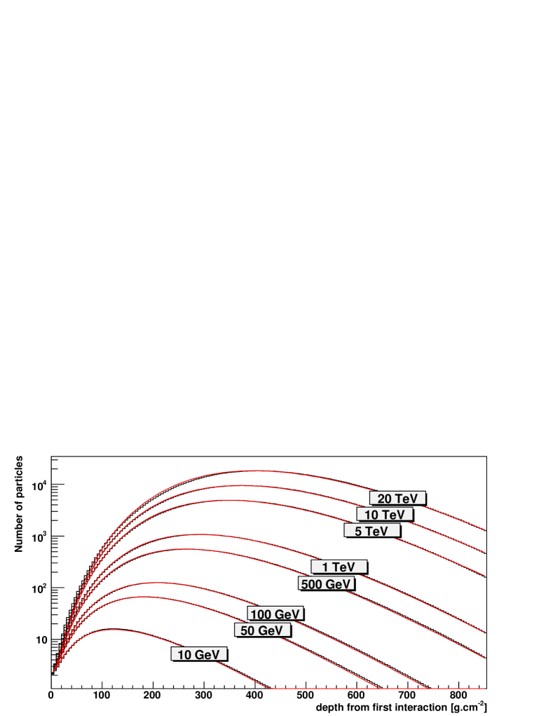
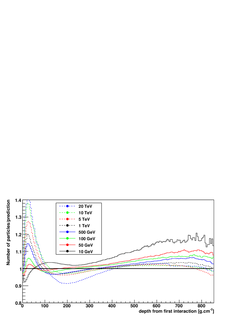
The average number of charged particles in simulated electromagnetic showers as a function of the distance to the first interaction point for different primary photon energies are shown in fig. 1. The longitudinal distributions are modelled by a modified Greisen formula[11]:
where is the scaled primary photon energy with being the primary photon energy and being the critical energy ( in air). The first part of the expression corresponds to the standard Greisen formula, with parameters and left free. The second part describes the decay of the two charged particles created at the first interaction point and ensures . The shower depth is given in units of radiation lengths. The shower age measured from the point of the first interaction is given by
| (1) |
This expression is constructed so that the shower age being at the first interaction and at the shower maximum. The parameter is the depth of shower maximum measured from the first interaction ( for ) and is a scaling factor related to speed of the shower development. The parameters and are found to be linearly dependent on the scaled energy . A fit of the analytical description on the simulated distributions yielded for the parameters , and :
| (2) |
As can be seen in fig. 1 the analytical description is in good agreement (at a level of in the central depth range, degrading to in the shower tail and in the shower head) with the simulation for primary energies ranging from to more than ,with slightly worse performances at the very high and very low energies.
The Cherenkov light distribution of an electromagnetic shower depends on the energy dependent longitudinal distributions of charged particles in the shower with
| (3) |
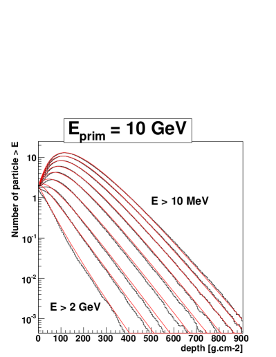
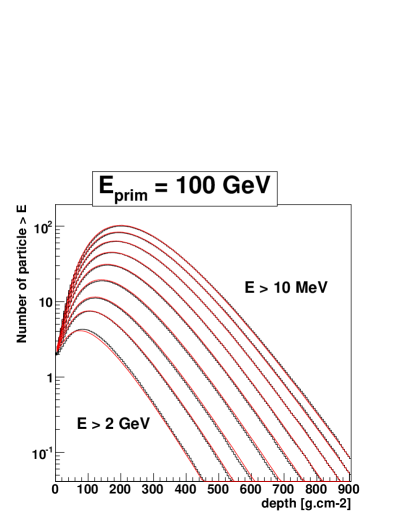
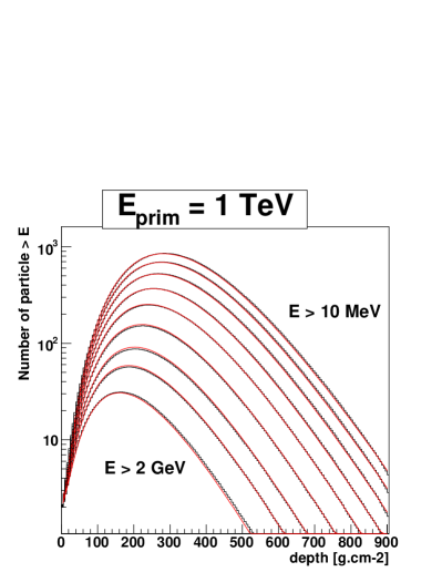
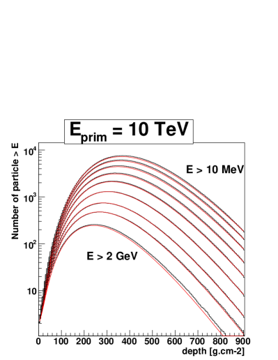
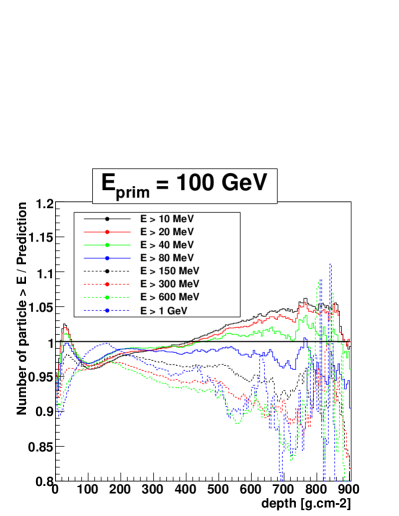
Examples of the longitudinal distributions of charged particles in the shower integrated over charge particle energy above some threshold (10 MeV, 20 MeV, 40 MeV, 80 MeV, 150 MeV, 300 MeV, 600 MeV, 1 GeV and 2 GeV) and for different primary photon energies is shown in Fig. 2 . The distributions are modelled using the same analytical expression as in Eq. 1.1 but with a different set of parameters:
| (4) | |||||
where is the charged particle energy, expressed in MeV.
 |
 |
 |
 |
 |
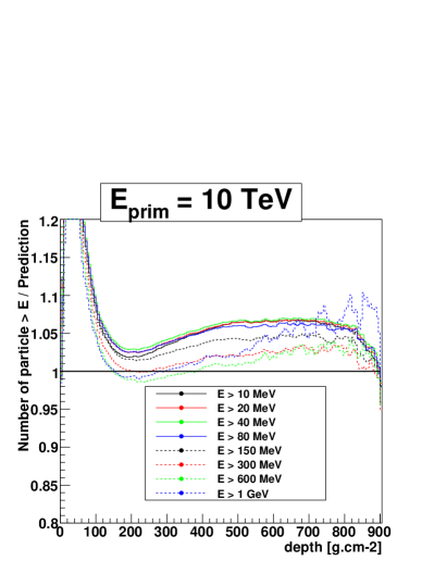 |
The comparison of the analytical function with the distributions from simulations with different primary energies is shown in Fig. 2. The agreement is very good (at the level of ) up to particle energies of a few GeV above which the particles contribute very little to the overall Cherenkov light distribution.
1.2 Angular distribution of particles in a shower
The angular distribution of charged particles in the shower together with the velocity dependent Cherenkov-angle determine the angular distribution of the Cherenkov-photons. As described in Moliere theory, the relevant angle of the charged particles is the reduced angle given as
| (5) |
where is the angle between the direction of the primary particle and the direction of the charged particle of energy in the shower. The angular distribution of the charged particles in the shower is decomposed into the mean reduced angle as a function of the particle energy of the charged particle and the distribution of reduced angles around the mean reduced angle.
The mean reduced angle is found to depend only very weakly on the primary particle energy and is parametrised by
| (6) |
The mean reduced angle for different primary particle energies as a function of the charged particle energy in units of the primary particle energy together with the parametrisation is shown in Fig. 3. There is a good overall agreement within a few percent between the mean reduced angle from the simulation and the parametrisation, in the range of small kinetic energies compared to the primary particle energy. Fig. 3 right shows the ratio between the simulation and the parametrisation. A deviation is seen when the charged particle kinetic energy exceeds about of the primary particle energy (corresponding to a red vertical line in fig. 3, right), affecting only a very small fraction of the particles in the shower.
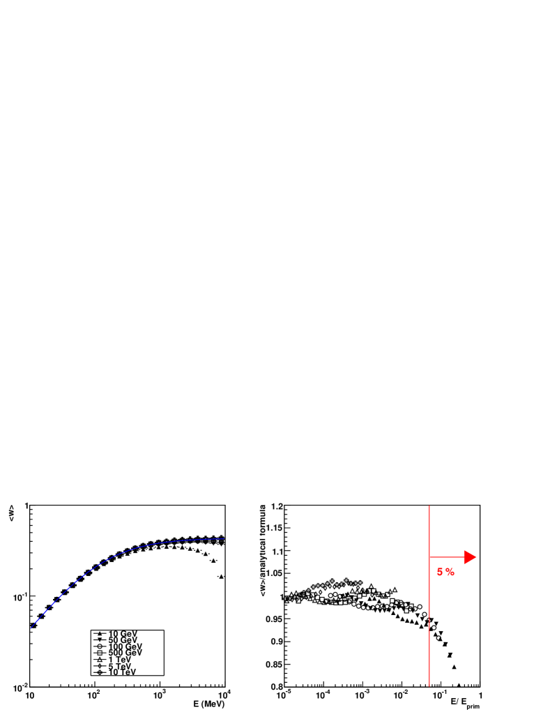
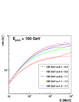
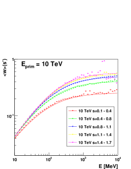
The detail modelling of the Cherenkov light distribution in a shower requires the dependency of on the shower age to be taken into account. The parametrisation of eq. 6 is kept, but with parameters varying with shower age:
| (7) |
The parameters , and are given by (fig. 4):
| (8) | |||||
 |
 |
 |
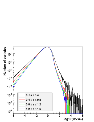
The distribution of angles around the mean is found to be quite independent of shower age or primary particle energy. The rescaled angle is used here:
| (9) |
The distribution of for varying shower age and particle energy is shown in fig. 5, and is found to be almost independent of these parameters. There is a slight broadening of the distribution at small shower ages, but this corresponds to the beginning of the shower when the number of charge particles is small.
 |
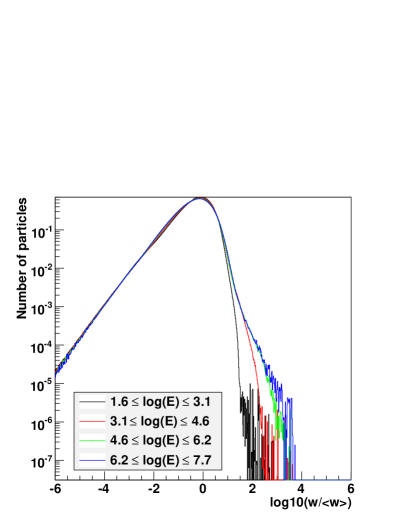 |
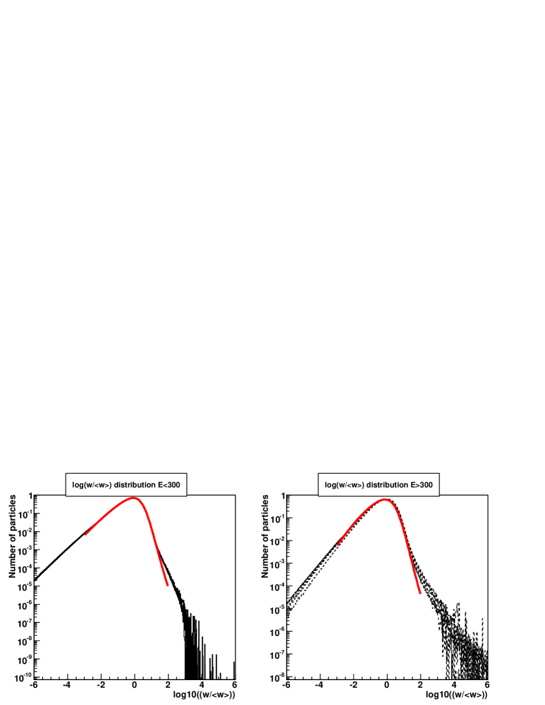
The distribution of , assumed to be independent of shower age or primary particle energy, is shown in fig. 6 and can be modelled by the expression111there was a typo in published paper
| (10) |
with:
| for | |||||
| for | (11) |
The distribution for different primary energies and for charged particles energies (left) and (right) is shown in fig. 6 with the analytical formula from eq. 10 superimposed (solid red line). A good agreement up to a few is observed in the central part of the distribution, encompassing the majority of particles in the shower.
1.3 Lateral distribution of particles in a shower
 |
The lateral distribution of the charged particles (electron or positron) in a shower are given in a system of coordinates attached to each charged particle in the shower as introduced in [10]. The -direction is defined as the projection of the particle flight direction on the plane perpendicular to the shower axis, and the direction is perpendicular to it (and therefore perpendicular to the particle velocity) (see fig. 7). The mean particle displacement with respect to the shower axis along the axis is non-zero, whereas the average displacement along the axis is zero for symmetry reasons.
Assuming a factorisation of the expressions of mean displacement and spread in terms of energy, particle angle and shower age, the following expressions are found to properly describe the particle spread (expressed in units of )222In the publised paper, eq 1.3 had a typo.:
| (14) | |||||
The above expression is a good description of the mean lateral displacement and spread at the level of 10%.
The reduced variables and are used for simplicity:
| (16) |
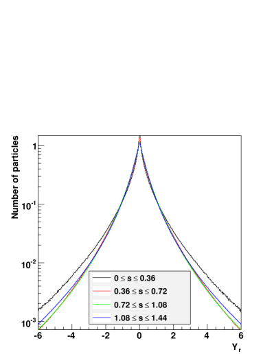
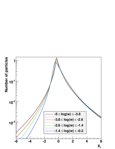
were , and are obtained from eq. 1.3 to 1.3. The distributions of and for 1 TeV gamma-ray showers are shown in fig. 8. The average values and RMS of and are respectively and , as expected if equations 1.3-1.3 are correct. As expected, the distribution is symmetric while the distribution is not.
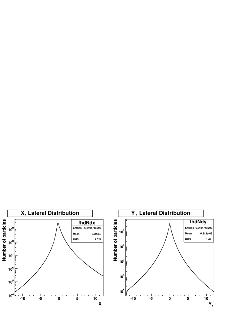
The distributions can be modelled by the following expression:
| (17) |
A similar expression can be derived for taking into account the non-centred position of the distribution maximum, and with different coefficients on both sides. For the sake of simplicity, a tabulated version of this distribution is used in the model production instead of a complicated analytical expression.
 |
 |
 |
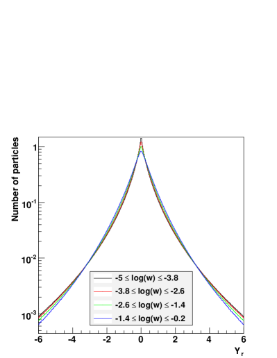 |
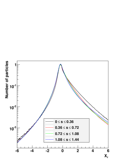
The dependency of the reduced and lateral distributions with shower age and particle angle is shown in fig. 9. The and distributions remain stable enough to be considered as independent of these parameters in the shower modelling. The small variation seen in the distribution of with particle angle affects mainly particles with a very large angle which are anyhow not likely to reach the telescopes.
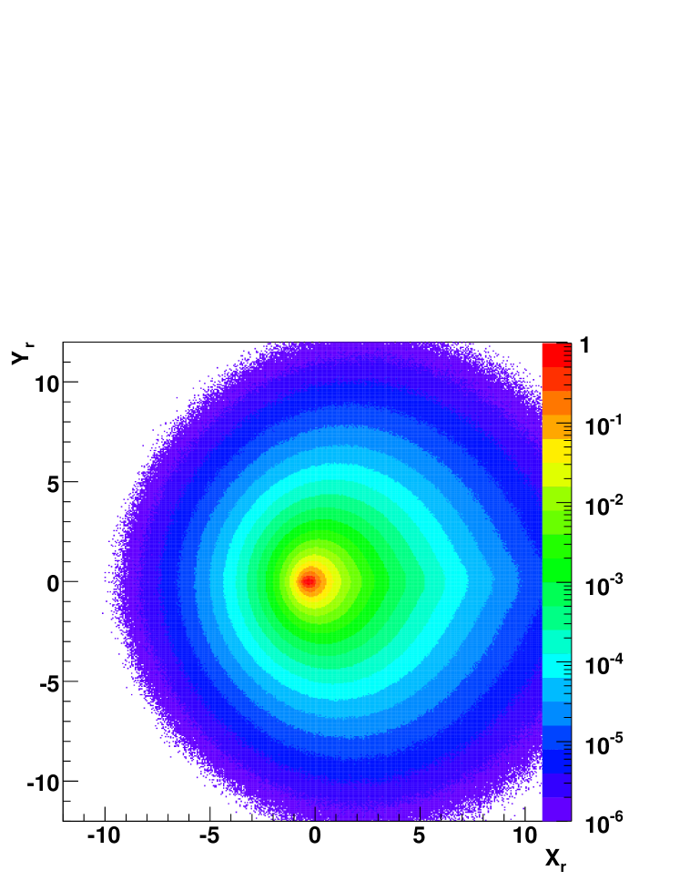
Figure 10 shows that the and distributions are mostly uncorrelated and can therefore be considered as independent.
2 Model Generation
The semi-analytical description of shower development described in the previous section can be used to construct a shower model, i.e. a prediction of the light distribution on the ground for a given primary particle energy, direction, impact parameter and development depth. This section describes how the shower image model is constructed from the distributions derived in the previous section.
2.1 Principles
The light density due to a shower in the camera can be calculated by an eight-fold integral:
-
•
integral over altitude or depth (longitudinal development of shower).
-
•
integral over energy of the electron/positron in shower.
-
•
integral over electron direction with respect to the telescope ( and ).
-
•
integral over electron position with respect to its direction ( and ).
-
•
integral over Cherenkov photon wavelengths.
-
•
integral over Cherenkov photon azimuthal angle around the electron (the angle between the electron and the Cherenkov photon being fixed for a given electron energy).
Where:
- •
- •
- •
-
•
is the Cherenkov photon production rate (per unit of vertical track length and emitted photon wavelength) for an electron angle with respect to the shower axis
-
•
is the atmospheric absorption
-
•
is the detector quantum efficiency (multiplied by mirror reflectivity and other wavelength-dependent transmission coefficients in the detector)
-
•
is the average geometrical collection efficiency for photons emitted by a electron at position with direction defined by , and with an azimuthal photon angle around the electron.
In addition to the aforementioned ingredients, instrumental effects such as instrument point spread function and electronic response of the camera, including in particular trigger response and integration duration, have to be taken into account in the calculation.
These effects, as well as the geometric light collection efficiency are obtained from a detailed simulation of the telescope response and parametrised in look-up tables. Atmospheric absorption of light, wavelength-dependent quantum efficiency and reflectivity used in the model generation are also implemented as look-up tables.
 |
In practice, for a given set of parameters, the relevant altitude range (in which emitted photons can reach the telescope) is first determined. Within this range, the shower development is divided into altitude slices (typically 20 slices). For each slice, the total number of charged particles in the shower is computed from eq. 1.1, and the particles are distributed in energy bands using eq. 4. For each energy band, the average energy, Cherenkov photon emission angle and emission yield (integrated over atmospheric transmission, quantum efficiency and dish reflectivity) is derived. The average shower is then further divided into flying particle angular bands and lateral displacement (eq. 6 to 17). For each considered position and direction, the geometric collection efficiency is then taken into account to compute the contribution of this small shower subset. At each calculation step, a precise estimation of the required integration range is performed to avoid spending too much time in sampling parts of the shower whose Cherenkov light do not reach the telescope mirror.
An example for such a determination (using a geometrical construction) is shown in fig. 11: The projection plane (ground) is taken perpendicular to the shower axis, which is assumed to intersect the ground at point . In order to avoid correlations with electron position and direction, the azimuthal range is determined in the shower direction frame (i.e. for a fixed shower and a telescope moving around the shower). The electron, at a fixed altitude , with an energy , is assumed to be at a distance with an angle from the shower axis. Point in the figure is the projection on the ground of the electron position. Its impact on the ground lies on the circle of radius around the point . Any Cherenkov photon emitted by this electron (with an angle with respect to the electron) will fall within the ring defined by the radii and . Intersections of this ring with the possible telescope position (circle centred on ) given the allowed azimuthal range . A similar approach is used to define the integration range for the other variables.
2.2 Parameter space
Models are generated for:
-
•
40 different zenith angles
-
•
40 impact distances ranging from to from telescope
-
•
65 different energies from to
-
•
6 first interaction depths from to .
The shower images are always generated on-axis (i.e. for a -ray at the centre of the camera). For a perfect telescope, a change of direction will result in a simple translation in the camera frame, that can be applied later, in the fit procedure. In a more realistic telescope, the broadening of the point spread function at large off-axis angles needs to be taken into account. This is currently not needed for the H.E.S.S. telescopes, which use a Davis-Cotton optical design offering a degradation of the PSF from 0.25 mrad (RMS) at the centre to 1 mrad at the edge of the field of view, however always smaller than the pixel size[12]. In total, templates are generated. The model generation procedure requires about 50 to 100 day-machine computing time on recent desktop computers and can be easily parallelled. The resulting shower images are stored in a ROOT binary file[13] for later use.
2.3 Example
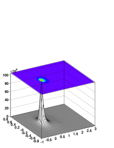
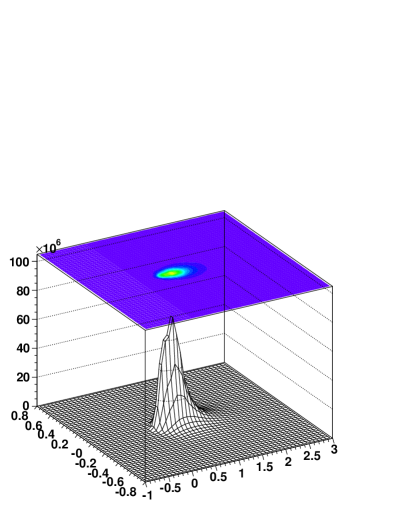
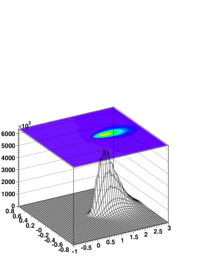
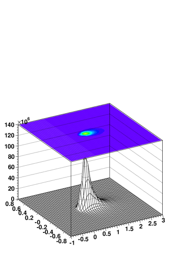
The output of the model generation procedure is a bank of two dimensional shower images in the frame of a perfect camera, with very small () pixel size. For a given primary particle set of parameters, a predicted image is computed with an interpolation procedure on the generated images in a 4 dimensional space (energy, impact distance, primary interaction depth and zenith angle). Shower direction and azimuthal angle are then taken into account as a rotation and a translation in the camera frame to compute the final predicted image. Examples of such two dimensional shower images are shown in fig. 12
 |
 |
 |
 |
2.4 Comparison with simulation
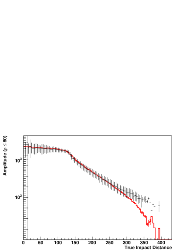
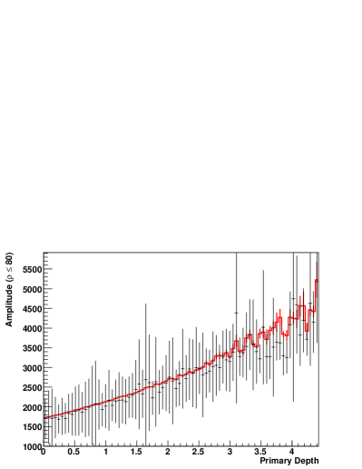
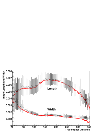
A comparison of the image shapes between simulation and model prediction is shown in fig. 13 for 1 TeV gamma-ray showers. The images were calculated for a H.E.S.S. camera, with pixels of diameter. The image length and width were estimated using the standard Hillas parametrisation applied to the predicted images. In each plot, the average value of the simulation is drawn as a black histogram, with error bars indicating the shower-to-shower fluctuations. The model prediction (image of average shower) is represented by a solid thick red line.
 |
 |
 |
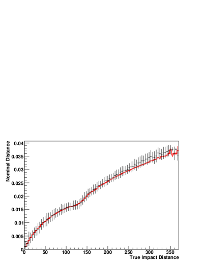 |
The agreement between the model and the average values of the simulation is excellent up to core distance of about 300 m, where some trigger effects can explain the differences: at this distance, the total image amplitude does not exceed 100 photoelectrons, distributed over many pixels. Showers fluctuating up to higher intensities are more likely to trigger the telescope, thus resulting in a higher average image amplitude in the simulation compared to the model.
The bars in the simulation histograms (in black) are due to shower-to-shower fluctuations, which are not taken into account in the model generation. At small core distance, and when taking into account the evolution with primary interaction depth, the shower intensity fluctuates by about 20% from shower to shower in addition to the fluctuation related to the depth of first interaction.
2.5 Conclusions
The work presented in this section results in the generation of a shower image model, which is nothing more than an accurate prediction of the expected Cherenkov light distribution in the camera for a given set of primary particle parameters. The key ingredients in the model generation are the inclusion of depth of first interaction as shower parameter (as the main source of shower-to-shower fluctuations), and the precise description of longitudinal, lateral, and angular distributions of charged particles in the shower. The corresponding shower model is constructed once for all and can be applied to various zenith angles, telescope impact distance or off-axis angle.
An alternate brute force approach would be the generation of the shower image model from massive simulations performed at every energy, zenith angle, impact distance, off-axis angle and primary interaction depth. The size of the parameter space and the need for a smooth model (in order to avoid local minima that would hamper the quality of the fit procedure) makes this approach less effective that the generation of an intrinsically smooth shower model.
3 Fit procedure
Once a shower model has been obtained, actual images on the camera can be compared to the ones predicted by the shower image model for a given set of primary parameters. A minimisation procedure is then used to obtain the most likely parameters of the incoming particle (energy, direction, impact, depth of the first interaction) under the hypothesis that the particle is a -ray. The minimisation procedure involves a precise comparison of the intensity in each pixel of the camera with the prediction from the model (interpolated between grid points to the actual set of parameters). In order to take into account the Poisson nature of the detected number of photons in each pixel, a log-likelihood approach has been chosen.
3.1 Pedestal and calibration
In the absence of Cherenkov light, each pixel of the H.E.S.S. camera is illuminated by a significant amount of Night Sky Background (NSB) light, which largely dominates over the electronic noise and represents a single photoelectron rate ranging from off the galactic plane to in the most luminous parts of the galactic plane. The pedestal is defined for each pixel as the charge distribution collected in the absence of Cherenkov signal. It is determined[14] for each pixel and for each observation run, using a cleaning procedure that identifies the position of the shower image in the camera and rejects the corresponding pixels. The pedestal width is the combination of the electronic noise and the night sky background, the later being largely dominant. Due to varying atmospheric conditions, rotation of the sky on the camera333The H.E.S.S. telescope use a Alt-Az mount and instrumental effects that depend on particular on temperature, the pedestal position and width can vary with time, with timescales of the order of a few minutes. The evolution of pedestal position and width with time for each pixel is recorded for every observation run and used during the reconstruction describe below.
3.2 Pixel log-likelihood
The shower image model provides a density of Cherenkov light in the focal plane. A convolution by the pixel size is done when loading the model to compute the expected signal in each pixel. For the sake of simplicity, the dependence of the PSF across the field of view is not taken into account in this calculation. The probability density (likelihood) to observe a signal of (in units of photoelectron) in a pixel for an expectation value is given by the convolution of the Poisson distribution of the photoelectron number with the photomultiplier resolution. The latter is well represented by a Gaussian of width where is the width of the pedestal (charge distribution under pure noise, including night sky background) and the width of the single photoelectron peak (photomultiplier resolution):
| (20) |
In eq. 20, the actual pedestal width is different for each pixel, and depends in particular on the level of night sky background (NSB) seen by the pixel. The photoelectron resolution , also specific to each pixel, is measured using calibration runs where the camera is illuminated with a low intensity flashing LED. The use of measured values of and is an important aspect that will explain the stability of the Model Analysis for varying level of NSB (Section 4.12).
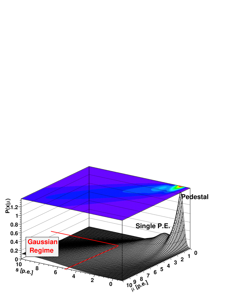
The shape of function 20 is shown in fig. 14. In order to obtain a variable that behaves asymptotically like a , we define the pixel log-likelihood
| (21) |
3.3 Pixel log-likelihood expectation values
In order to compare the observed signal with a model prediction , the expectation value of the log-likelihood under different realisations of the same shower image (i.e. being fixed and fluctuating due to Poisson noise, electronic and NSB fluctuations) needs to be computed. If the observed signal is only due to noise (night sky background), the probability density functions simplifies to a Gaussian of width . In this case, the average value of the pixel log-likelihood reads
| (22) | |||||
In a similar manner, one obtains
| (23) |
At high , the Poisson distribution can be replaced by a Gaussian of width , and the probability density function can be well approximated by the convolution of two Gaussian:
In this limit, the log-likelihood behaves like a :
| (24) |
This expression reduces to eq. 22 when . Figure 15 shows the comparison of this analytical expression with a numerical integration of the average log-likelihood. The analytical expression is valid for and, as expected, is also asymptotically valid for . In the transition regime, the analytical expression slightly overestimates the likelihood value.
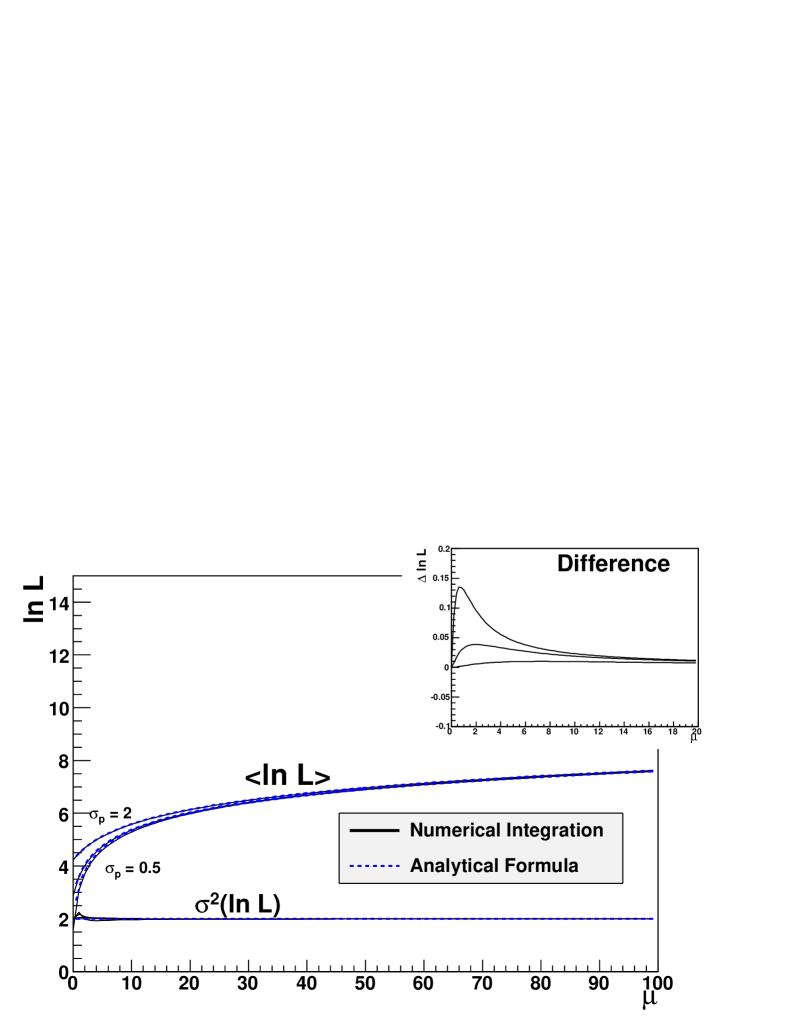
In order to properly calibrate the average log-likelihood, the discrepancy between the analytical expression and the numerical integration is computed for every expected amplitude and pedestal width (using a Monte Carlo simulation) and stored in a look-up table. This look-up table will be used at the end of the fit procedure (see below) to produce calibrated discriminating variables.
3.4 Telescope log-likelihood
Pixels belonging to a camera are assumed to be independent. We define the telescope log-likelihood as the sum over all pixels of the pixel log-likelihood:
| (25) |
3.5 Reconstruction - Fit algorithm
The model photon reconstruction relies on the pixel-per-pixel comparison of the actual shower images with the ones that are predicted for a given set of parameters. A minimisation procedure is used to find the best parameters (direction, impact, depth of the first interaction and energy). In contrast to Hillas parameters based reconstruction techniques, the raw image amplitudes are directly used, without any image cleaning procedure. All pixels are used in the fit, not only those close to the actual image.
A Levenberg-Marquardt fit algorithm [15, 16] is used to minimise the telescope log-likelihood (eq. 25). This algorithm is very efficient in the case the first and second derivative of the minimised function (log-likelihood or ) can be expressed analytically and depend mostly on the first derivative of the model (the second derivative being negligible). This is in general valid when the minimised function is a quadratic form ( or similar) and when the model function exhibits a smooth behaviour when varying the model parameters. The algorithm assumes a quadratic form and uses the inverse matrix of second derivatives to estimate the position of the minimum. In order to improve convergence stability, a combination of pure steepest descent and parabolic assumption is used with weights that vary during the minimisation, depending on whether the quadratic assumption is valid or not. The Levenberg-Marquardt fit algorithm always converges - sometimes to a local minimum - and provides reliable estimates of the model parameters uncertainties, taken from the correlation matrix.
An important issue in the fit algorithm is the starting point. The standard Hillas reconstruction technique[17] with different sets of image cleaning parameters is used to derive a handful of possible estimates. The estimate that provides the best initial log-likelihood is chosen as starting point of the minimisation.
In our case, about 40 iterations are needed for the algorithm to converge, whereas simpler algorithms such as Minuit[18] needed in average about ten times more. On recent desktop computers, the reconstruction of a single event takes about to .
The actual telescope reflectivity, as measured from ring-shape images of muons passing through the telescope[14], is used to scale the model prediction to the observation conditions, on a run-by-run basis. Since the optical efficiency is taken into account directly at the reconstruction level, no further energy correction is needed (which is completely different to the way the optical efficiency is handled in Hillas parameters based analyses).
The output of the minimisation procedure are:
-
•
Best guess of the 6 shower parameters: direction (2 parameters), impact (2 parameters), depth of the first interaction and energy
-
•
Correlation matrix and therefore uncertainty on these best fit parameters
-
•
Final log-likelihood value
3.6 Goodness of fit
Since Atmospheric Cherenkov Telescopes are background dominated systems, the performance of any analysis is mainly driven by its ability to discriminate between gamma-ray induced showers and the much more numerous hadronic background. In the Model Analysis, a goodness-of-fit approach is chosen to compare the model prediction and the actual shower images, in order to check the compatibility of the recorded events with a pure -ray hypothesis. The goodness-of-fit is defined as a normalised sum over all pixels of the difference between the actual pixel log-likelihood and its expectation value, properly normalised:
| (26) |
where is the number of degrees of freedom (number of pixels - 6). The goodness of fit behaves asymptotically like a and provides therefore a measure of the fit quality. This will be used later on the hadronic discrimination. By construction, if the pixels likelihood behave like independent random variables, is expected to behave like a normal variable:
| (27) |
3.7 Goodness of fit calibration
The goodness of fit average value relies on the assumption of a Gaussian pedestal (of width ). In the absence of night sky background, the pedestal reduces to the electronic noise and the assumption is always valid[14]. The H.E.S.S. camera use two different gains: a high gain, with dynamical range from 0 to 200 photoelectrons with single photoelectron resolution and an electronic noise representing about p.e., and a low gain, with dynamical range up to 2000 photoelectrons but worse resolution. In the low gain, where the electronic noise represents about p.e., the pedestal is also Gaussian to a good approximation.
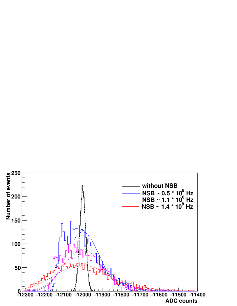
In the high gain channel, figure 16, reproduced from [14], shows that the Gaussian assumption is also almost valid for high night sky background (above ), but not in the intermediate regime where the pedestal shape exhibits two peaks, similar to a single photoelectron spectrum, and produced by fractions of single photoelectron pulses falling by chance within the acquisition window.
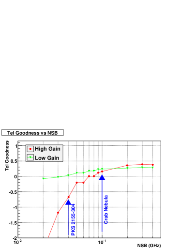
Simulation of -ray spectra were conducted with different levels of night sky background (from to ). Figure 17 shows the average goodness of fit, computed on a single telescope basis (to keep a constant number of pixels), and as function of the night sky background level for the two gains of the H.E.S.S. camera.
 |
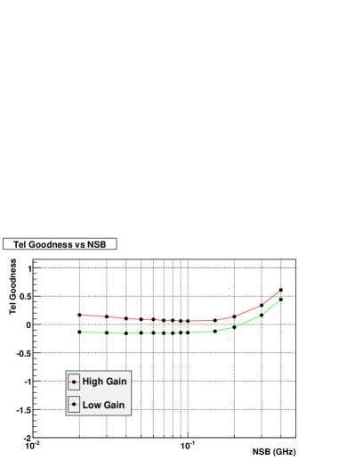 |
The goodness of fit calculated with low gain channels on each pixel appears to be rather stable with night sky background, thus confirming the validity of the Gaussian assumption for this channel. In contrast, the goodness of fit calculated with high gain channels exhibit a strong deviation at low night sky background level, where the pedestal is not Gaussian anymore. Simulations were used to derive a correction table as function of night sky background level in each pixel independently. This table is not used during the reconstruction, and is only applied to the final goodness of fit estimator. The resulting goodness-of-fit is shown in fig. 17, before correction (left) and after correction (right). After calibration, the goodness-of-fit is stable for a night sky background variation from to , which corresponds the bulk of the H.E.S.S. observations.
3.8 ShowerGoodness and BackgroundGoodness
The discrimination between -ray induced showers and hadron induced ones can use several distinct features (fig. 18):
-
•
Hadron induced showers are more irregular, and contain several electromagnetic sub-showers initiated in particular by disintegration of neutral pions. As a consequence, the image in a Cherenkov camera often exhibits several clusters separated apart (fig. 18, left)
-
•
In addition, the hadronic component of the shower itself emits a low intensity Cherenkov light spread over a large fraction of the camera. This emission, denoted as Hadronic rain, is in general eliminated by cleaning procedures used in standard reconstruction techniques. (fig. 18, middle).
-
•
Finally, the charged nucleus entering the atmosphere can emit a Cherenkov light before interacting. This emission is produced very high in the atmosphere and therefore it generates, in the camera, a faint spot close to the shower direction.
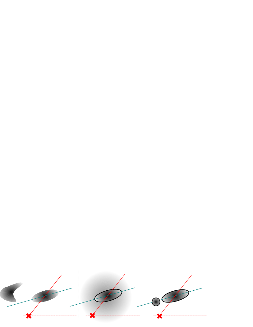
In order to fully exploit the differences between the and hadron induced showers, individual pixels contributing to the goodness-of-fit (eq. 26) are classified into two different groups at the end of the fit:
-
•
Pixels belonging to the shower core, defined as pixels whose predicted amplitude is above , are grouped together with three rows of neighbours around them to construct a variable named ShowerGoodness (SG) in a similar way to eq. 26. These pixels are selected at the end of the fit procedure to avoid changes of the number of degrees of freedom during the fit. Due to the large reduction of the number of degrees freedom, this variable is more sensitive than the Goodness to discrepancies between the model prediction and the actual shower images.
-
•
Remaining pixels, denoted as background pixels, are grouped together to construct a variable named BackgroundGoodness (BG), which is sensitive to hadronic clusters outside the main image, hadronic rains and other irregularities.
4 Results
4.1 Data sets
For a detailed comparison of the Model Analysis with previously existing reconstruction techniques, two data sets are used:
-
•
A data set (PKS Flare) of 7.7 hours (live time) of data taken on the blazar PKS 2155-304 during flaring period in July 2006, with 4 telescopes, yielding a test sample of more than 10 000 -rays with very small background contamination, at relatively low zenith angles (typically ). The average night sky background for this data set corresponds to a single pixel triggering rate of , representative for extragalactic space. Since the data has been taken within 3 days, the system state can be considered as stable.
-
•
A large set (Crab Full) of 34 hours (live time) of data taken on the Crab Nebula, from 2004 to 2008, with 4 telescopes and larger zenith angles (from to ). This data set yields a sample of excess events. The average NSB for this data set, representative for galactic plane, is more than twice higher () than for extragalactic space.
The model analysis will be compared to the standard Hillas parameters based reconstruction in use in the H.E.S.S. collaboration[17]. Two sets of cuts will be defined: Hillas 60 will denote a minimum image amplitude of 60 photoelectrons (p.e.), same as for the Model Analysis, and Hillas 200 will use a larger minimum image amplitude of 200 p.e.. When needed, Hillas Std and Hillas Hard will denote configurations used in the Crab publication[17] with respectively 80 and 200 p.e. minimal image amplitude.
4.2 Shape cuts
In order to have well reconstructed showers, the following shape cuts are used throughout the current section (unless specified differently):
-
•
A minimum image amplitude of 60 photoelectrons per telescope.
-
•
A maximal nominal distance (distance of the shower image centre to the centre of the camera) of for a camera radius of . The nominal distance cut removes truncated images, close to the camera edge, that often lead to misreconstruction of shower direction.
-
•
At least images from two different telescopes passing the previous cuts to ensure stereoscopic reconstruction.
These cuts will be used both for the Model Analysis and for the Hillas parameters based reconstruction techniques. The later needs an additional cleaning procedure. We use a two-level filter cleaning[17] with pixel thresholds of respectively and . The image amplitude is computed after cleaning. The Model Analysis doesn’t require any cleaning procedure, so the image amplitude for the model photon reconstruction is slightly larger than for the Hillas analysis (as pixels belonging to the shower image tail are taken into account for the model reconstruction and not for the Hillas reconstruction).
4.3 Hadron discrimination
 |
 |
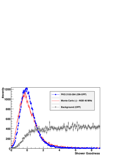
The distribution of ShowerGoodness (SG) in the shape cuts of section 4.2 is shown in fig. 19 for the data taken on the blazar PKS 2155-304, and for a simulation with 40 MHz of night sky background noise, corresponding to the average night sky luminosity around PKS 2155-304. The Monte Carlo distribution (red line) and the distribution for the PKS 2155-304 excess events (blue filled circles) are in overall good agreement, and are very different from the distribution obtained for background events (grey triangles), thus confirming the discrimination capabilities of the ShowerGoodness variable. The small shift between the two distribution is responsible for a systematic error in acceptance determination of 4% for a cut at .
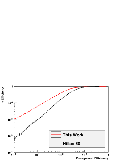
Fig. 19, right, shows the -ray efficiency as function of background rejection for a selection based on ShowerGoodness only444several other variables, described later in this paper, can provide additional rejection, after shape cuts, compared to what is achieved in the standard Hillas parameters based reconstruction (at the same minimal image amplitude, and using the Mean Scaled Width as varying selection variable). A large squared angular distance cut of was used to ensure that all events are accepted (extended source assumption) and to decorrelate angular resolution performance(sec. 4.8) from hadronic discrimination. The model reconstruction provides, for a given -ray efficiency, a much better background rejection than Hillas parameters based reconstruction. Moreover, as will be shown in the following sections, the Model Analysis provides additional discriminating variables that improve further the sensitivity.
In the standard configuration of the Model Analysis, a cut ShowerGoodness will be used as main discriminating parameter. This cut retains of -rays and rejects more than of background events, yielding a quality factor
| (28) |
4.4 Primary interaction reconstruction
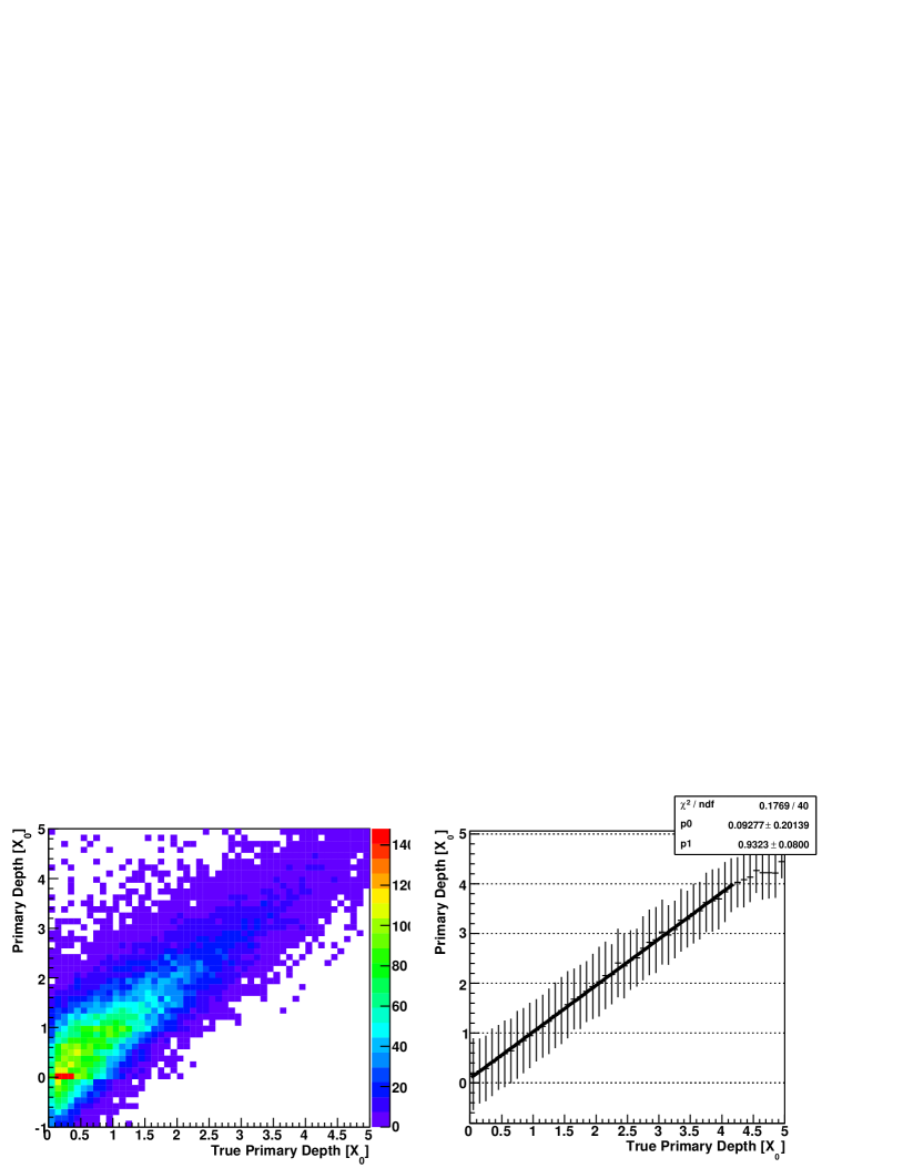
The depth of the first interaction being a parameter of the model, is also a direct product of the reconstruction procedure (instead of being calculated, as in the Hillas parameters based reconstruction, from the shower maximum). Fig. 20 shows the ability of the Model Analysis to reconstruct the depth of the first interaction with almost no bias and a resolution of (slightly worse at large zenith angles). This is better than Hillas parameters based analyses, which obtain resolution not better than in the best cases.
 |
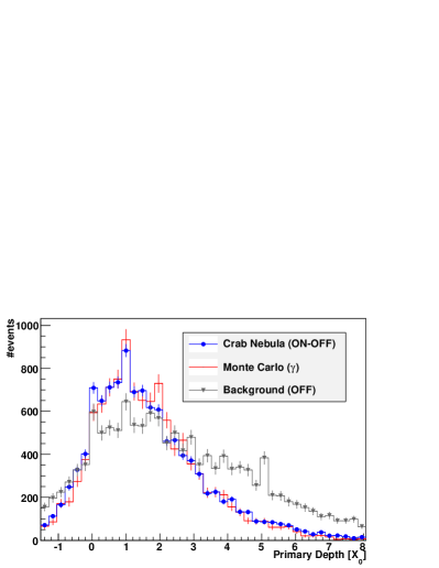 |
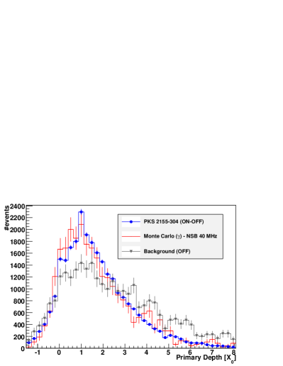
A comparison of the actual depth of the first interaction obtained with real data and with simulation is shown in fig. 21, in shape cuts and , under a point-like source assumption (squared angular distance cut of ). The agreement between data and simulations is excellent. The PKS 2155-304 data are compatible with a resolution, and the Crab data with a slightly worse () resolution due to a larger average zenith angle. Moreover, since the distribution for OFF data is significantly different, the depth of the first interaction can be used to improve the -hadron separation. The irregularities in the OFF distributions are artifacts of the reconstruction procedure: models are only available for depths of and and are linearly interpolated between these values (and extrapolated above ). Poorly constrained showers tend to accumulate at the grid model points and avoid interpolated values.
In order to improve -background separation, a cut in reconstructed primary interaction depth is used. This cut retains of -rays (resp.) and rejects of hadrons (resp. ) , yielding a quality factor (resp. ) respectively for the Crab and PKS 2155-304 data sets, leading to an improvement of the signal over background ratio by about .
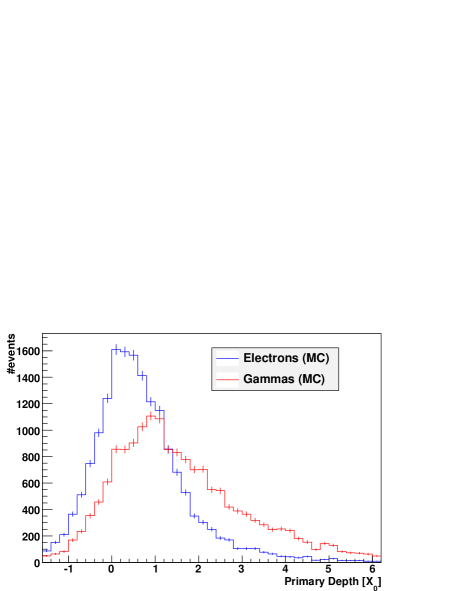
At low energies, the electron background becomes dominant for atmospheric Cherenkov telescopes. It is usually considered as irreducible, since electron induced showers are almost identical to -ray induced one. However, electron induced showers start to produce Cherenkov light a little bit earlier in the atmosphere (about a radiation length before ). This is confirmed by simulation shown in fig. 22: the distribution of reconstructed primary depth for a simulated electrons spectrum shows a peaks centred around , earlier than for ’s. The difference is not big enough to distinguish between electrons and gammas on an event by event basis, but a statistical discrimination seems to be possible.
4.5 Analysis Configurations
The -hadron separation is essentially based on the ShowerGoodness and primary interaction depth variables. For completeness, two additional cuts are used: a cut on BackgroundGoodness (), with -ray efficiency close to , is designed to remove a small number of shower misreconstructed at very large distance from the camera centre ( degrees or more). A second cut on the Goodness () variable (eq. 26), in which the model is replaced by a null () assumption, removes images that are consistent with pure night sky background noise, and reduces the effect of night sky background inhomogeneities across the field of view.
The standard cuts for the Model Analysis are defined as:
-
•
A minimum image amplitude of 60 photoelectrons per telescope
-
•
A maximal nominal distance (distance of the shower image centre to the centre of the camera) not more than
-
•
At least two telescopes passing the previous shape cuts
-
•
A maximum ShowerGoodness (SG) of
-
•
A reconstructed primary interaction depth between -1 and 4 .
-
•
For a point-like source, a squared angular distance cut of , independent of zenith angle555Since the angular resolution degrades at large zenith angle, a varying cut could perform better. This is not specific to the Model Analysis and applies to other reconstruction techniques as well.
Two additional sets of cuts are defined as reference point for future H.E.S.S. publications: the Faint source configuration is optimised for source fainter than a few percent of the Crab flux. The Loose cuts configuration is designed to maximise the -ray efficiency for strong sources at the expense of a poorer background rejection. For analysis of extended source, the cut is usually replaced by a selection that encompasses the whole source. Cuts for the three aforementioned configurations are summarised in Tab. 1. of cuts
| Name | Min. | Max. Nom. | #Tels | |||
| Charge | Distance | |||||
| (p.e.) | (deg.) | () | () | |||
| Standard | 60 | 2 | 2 | 0.6 | 0.01 | |
| Faint Source | 120 | 2 | 2 | 0.4 | 0.005 | |
| Loose Cuts | 40 | 2 | 2 | 0.9 | N/A | 0.0125 |
4.6 Effective Areas
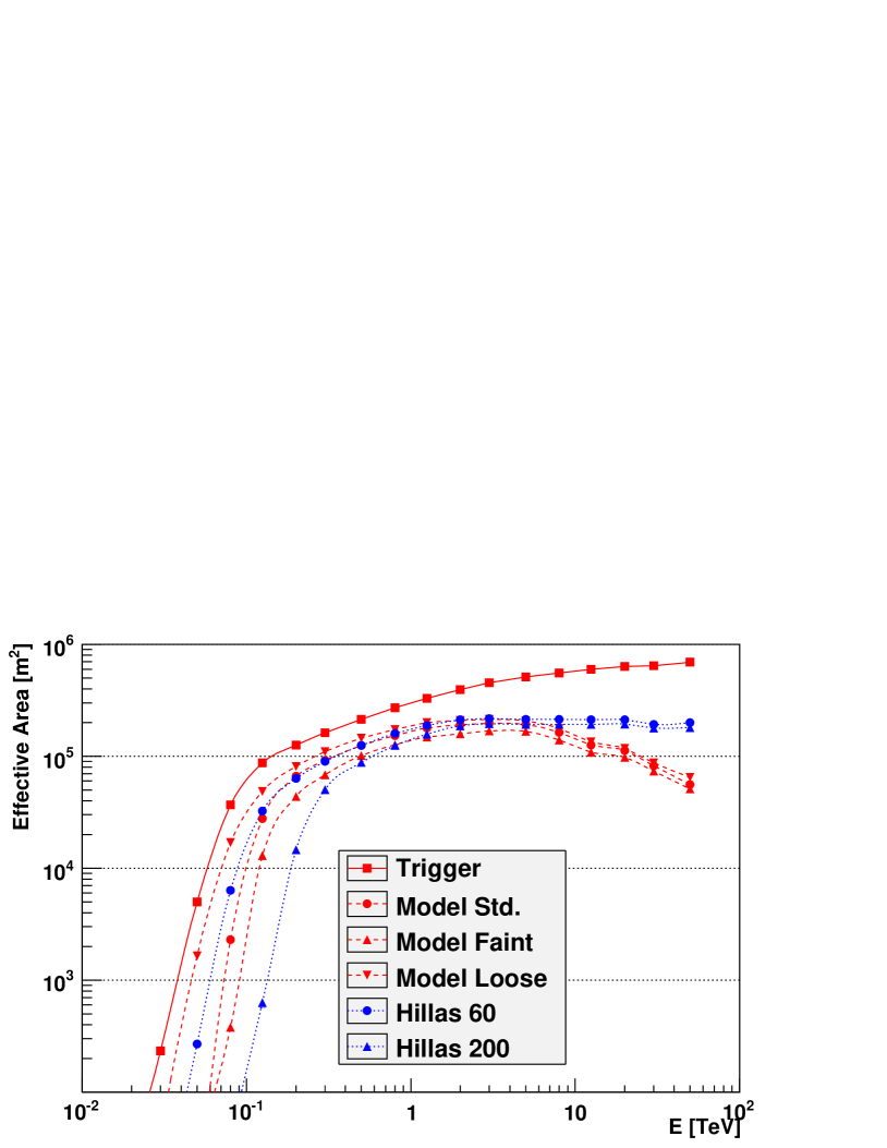
The effective area as function of energy for the Model Analysis at zenith is shown in fig. 23, compared to areas obtained with Hillas parameters based reconstructions. The reconstruction efficiency for the standard configuration is similar to the values obtained with Hillas reconstruction with a minimum image amplitude of 60 p.e.. As expected, the loose configuration has a larger effective area and a lower threshold. In most of the H.E.S.S. publications so far, a minimum image amplitude of 200 p.e. was used, yielding a much larger threshold of at zenith. Models are currently generated only up to , thus leading to a loss of acceptance at high energy. In addition, showers above can reach the ground, resulting into large fluctuations that are not fully reproduced by the model.
Performances obtained on the Crab Nebula and on the Blazar PKS 2155-304 are shown in tab. 2. The Model Analysis yields a -ray efficiency similar to the 60 p.e. Hillas reconstruction, but with a background rejection improved by a factor of (PKS 2155-304) to (Crab Nebular), yielding a signal over background ratio similar or better to the one obtained with hard cuts Hillas reconstruction. As a result, the significance obtained with the Model reconstruction is larger, and the sensitivity improved by a factor of more than . The faint source configuration provides an additional factor of in S/B compared to standard configuration.
| Data Set | Analysis | ON | OFF | S/B | |||
|---|---|---|---|---|---|---|---|
| Crab Full | Hillas 60 | 12768 | 26154 | 16.2 | 11148.6 | 162.6 | 6.9 |
| Crab Full | Hillas 200 | 3742 | 1435 | 16.9 | 3657.1 | 125.0 | 43.1 |
| Crab Full | Model Std | 10249 | 3848 | 18.2 | 10037 | 210.7 | 47.3 |
| Crab Full | Model Faint | 5920 | 1605 | 25.8 | 5857.7 | 176.8 | 94.0 |
| Crab Full | Model Loose | 20107 | 22137 | 16.7 | 18782.3 | 244.3 | 14.2 |
| PKS Flare | Hillas 60 | 24964 | 7025 | 10.9 | 24320.4 | 302.1 | 37.8 |
| PKS Flare | Hillas 200 | 5148 | 490 | 12.7 | 5109.3 | 153.9 | 132.1 |
| PKS Flare | Model Std | 24388 | 1303 | 12.7 | 24285.4 | 342.9 | 236.7 |
| PKS Flare | Model Faint | 11047 | 427 | 18.1 | 11023.4 | 248.1 | 466.5 |
| PKS Flare | Model Loose | 38308 | 3676 | 11.0 | 37972.7 | 407.2 | 113 |
4.7 Energy resolution
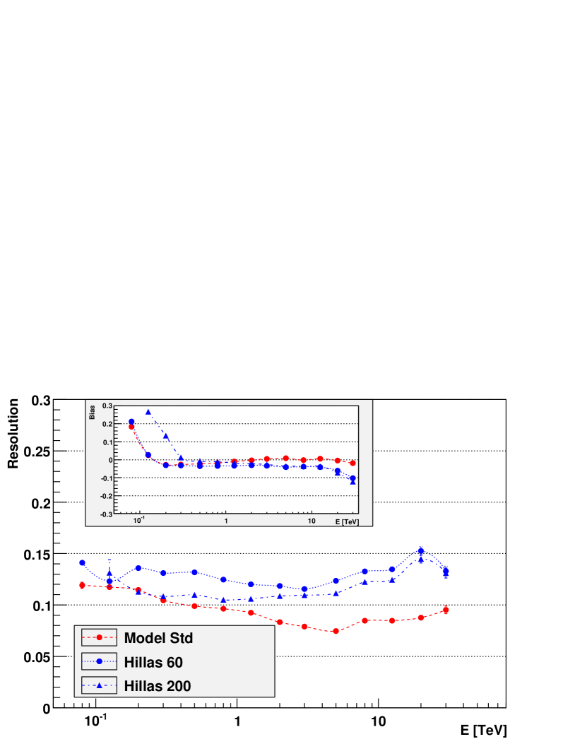
The energy resolution (in cuts) as function of energy is shown in fig. 24 for zenith, where the energy resolution is defined as the RMS of the distribution. The energy resolution is better than for the whole energy range (from up to more than ), with biases not exceeding in the central range. The very central energy range ( to more than ), the energy resolution is better than and reaches values as low as to . Larger energy biases appear at very low energy (up to at ), due to trigger selection effects. These biases are however smaller than those obtained with an Hillas parameters based reconstruction. In a similar manner, negative energy biases appear at very high energies, due to very distant high energy showers reconstructed closer to the telescopes666Very distant shower produce almost parallel images in the camera, which introduces a degeneracy in the reconstruction. and with an underestimated energy. In the medium energy range ( to a few 10 ), the Model Analysis largely outperforms standard reconstruction techniques.
4.8 Angular resolution
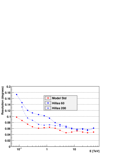
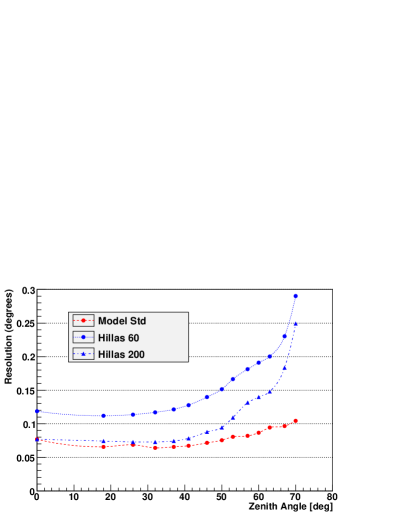
The angular resolution, defined as the containment radius, is shown in fig. 25 for showers at zenith (left), and is of the order of in most of the energy range, which is much better than values obtained with Hillas parameters based analyses (using algorithm 1 from [19]) for similar minimal image amplitude. An immediate consequence is an improved sensitivity for point like sources and improved morphological studies of extended source. The angular resolution is stable for zenith angles up to (fig. 25, right), ans rises slowly up to very large zenith angles. The degradation observed for very large zenith angles is much larger for Hillas parameters based reconstruction techniques.
 |
 |
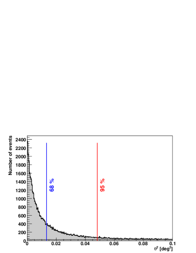
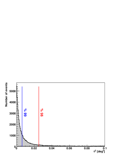
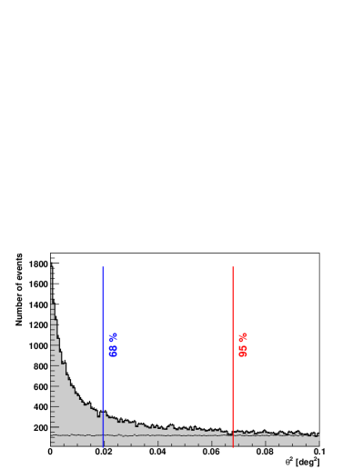
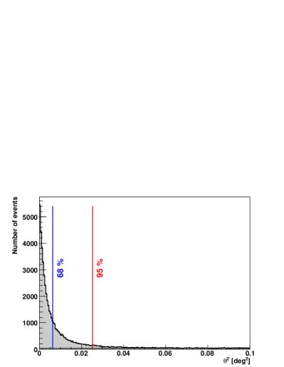
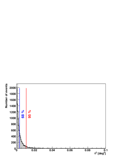
The superior angular resolution of the Model Analysis is demonstrated in fig. 26 on data taken on PKS 2155-304. The distribution is twice as more peaked for the Model Analysis (right), compared to the Hillas reconstruction (left). The same behaviour is observed at larger zenith angles for the Crab Nebula (fig. 27).
 |
 |
 |
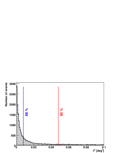 |
Detailed numerical comparison shown in tab. 3 demonstrates that, on average, the Model Analysis angular resolution performances with a minimal image amplitude of 60 p.e. are equally good as the Hillas Analysis with a much higher minimal image amplitude of 200 p.e..
| Data Set | Analysis | ||
|---|---|---|---|
| Crab Full | Hillas 60 | 0.14 | 0.26 |
| Crab Full | Hillas 200 | 0.09 | 0.21 |
| Crab Full | Model Std | 0.09 | 0.22 |
| PKS Full | Hillas 60 | 0.11 | 0.22 |
| PKS Full | Hillas 200 | 0.07 | 0.14 |
| PKS Full | Model Std | 0.08 | 0.16 |
4.9 Uncertainty on parameters
The Model Analysis provides uncertainty estimation for each reconstructed parameter, as byproducts of the correlation matrix. This can be used to select in a simple and natural way a sub-sample of the events with improved angular or energy resolution (for more precise morphological or spectral analysis).
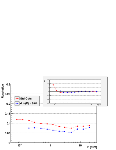
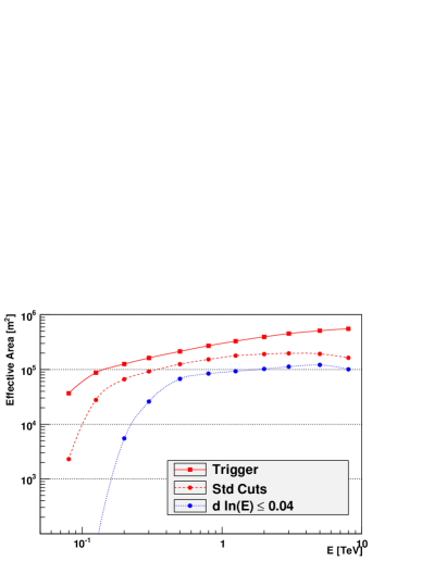
An example of such a subset selection is shown in fig. 28, where an additional selection on the energy uncertainty is applied to the data. The energy resolution becomes better than from up to with values as low as at a few . The prices to pay for such a golden events selection is an increase of energy threshold and a reduction of statistics (fig. 28, right) by a factor of above .
 |
 |
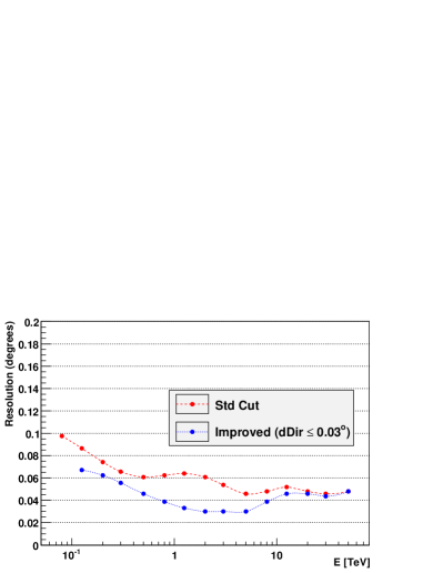
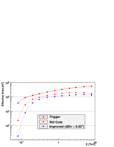
In a similar manner, fig. 29 shows the effect of an additional selection on the direction uncertainty on the angular resolution. It is possible to achieve a resolution as good as in the TeV energy range at the expense of a factor less than 2 in statistics. This can greatly improve the ability to pin-point the source position in challenging regions such as the Galactic Centre.
 |
 |
This is demonstrated in fig. 30, where the same selection is applied to data from PKS 2155-304. The net result of the selection is an unprecedented resolution and with number of excess event being still around 10000 . The background is also much more suppressed than the signal, resulting into a ratio of compared to before selection. The direction uncertainty could therefore serve as an additional discriminating parameter, but its effect would not be independent of energy.
 |
 |
4.10 Combination of reconstruction methods
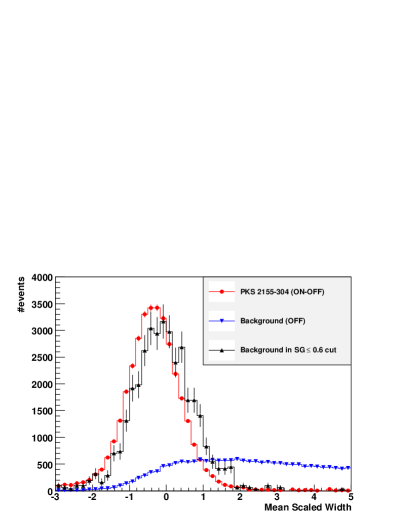
In the early stages of the Model Analysis, it was realised that the Goodness variable was almost uncorrelated with the Mean Scaled Width and Mean Scaled Length variables obtained with standard reconstruction techniques[20, 21]. As a consequence, the combination of several reconstruction techniques was improving rejection capabilities and thus final sensitivity.
 |
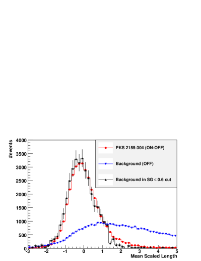 |
Fig 31 shows the behaviour of the Mean Scaled Width and Mean Scaled Length variable (from Hillas reconstruction) when imposing the ShowerGoodness cut. The background data histograms (in blue) are much more extended than the excess events (-rays) histograms (red), thus confirming the rejection capabilities of the Mean Scaled Width and Mean Scaled Length variables. However, after imposing a selection on the ShowerGoodness (), most of the discrimination capability vanishes (black histograms): the Mean Scaled Width still provides only a very small additional discrimination, whereas the Mean Scaled Length does not anymore. The games of combining several analyses appears therefore not as promising as it was, when using a older version of the Model Analyis with less performance.
4.11 Sensitivity to stars and broken pixels
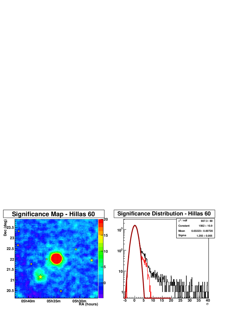
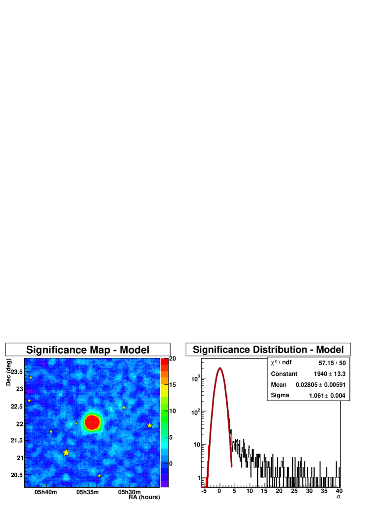
During H.E.S.S. observations, camera pixels illuminated by a bright star are turned off to avoid damage to the photocathode. In addition, some (in general less than ) pixels are removed from the analysis due to instrumental malfunction (non working high voltage, noisy pixel, badly behaving analogue memory, …). Missing pixels affect more Hillas parameters based analyses (as they produce truncated images) than the Model Analysis, which just ignores the missing pixels.
The effect of bright stars is demonstrated in fig. 32, where the large Crab Nebula data set (32 live hours) was used to produce a significance map using the template model[22]. A bright star, -Tauri of visual magnitude 2.97, is present in the field of view. On average, about three to four pixels surrounding the star are turned off during observations. An artificial excess of events, up to the level of , is visible in the Hillas Analysis significance map. This excess is due to a deficit in background events which translates into an artificial excess of events. The Model Analysis significance map shows no deviation at the same position, demonstrating that it is less sensitive to missing pixels. The artifact in the Hillas Analysis significance map weakens at larger minimal image amplitude (200 p.e.) as the shower images in the camera become larger and are therefore less affected by a few missing pixels.
4.12 Sensitivity to varying night sky background
 |
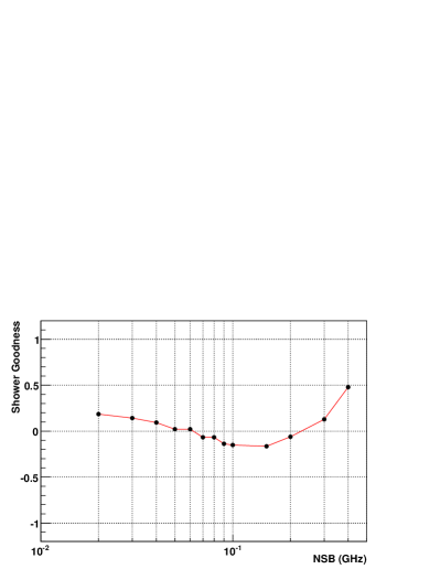 |
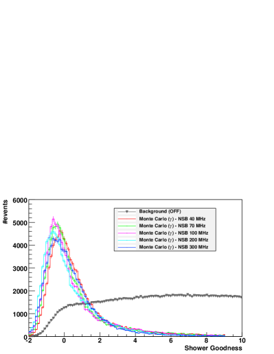
The evolution of Shower Goodness distribution for simulated -rays (with photon index 2.0 at zenith) is shown in fig. 33. No strong evolution is seen up to . The bulk of the HESS observations correspond to an average NBS level of , varying between to in the most luminous parts of the Galactic Plane.
Conclusion
We have presented a sophisticated -ray reconstruction technique for Atmospheric Cherenkov Telescopes, based on an accurate pixel per pixel comparison of observed intensity with a pre-calculated model. This significant improvement over earlier works leads to an improved angular and energy resolution, and background rejection, resulting in an increase of the sensitivity of the H.E.S.S. telescope system by a factor close to 2. The model analysis is less sensitive than reconstruction techniques based on Hillas parameters to instrumental or environmental effects (missing pixels, night sky background variation across the field of view, …), thus allowing an optimal use of the full dynamical range of the instruments. This novel reconstruction technique should also benefit to upcoming projects such as CTA and AGIS.
Acknowledgements
We thank Prof. W. Hofmann, spokesman of the H.E.S.S. Collaboration and Prof. G. Fontaine, chairman of the Collaboration board, for allowing us to use H.E.S.S. data in this publication. We are grateful to Dr. B. Degrange and Prof. C. Stegmann for carefully reading the manuscript and for providing us with very useful suggestions. Finally, our thanks go to all the members of the H.E.S.S. Collaboration for their technical support and for many stimulating discussions.
References
- [1] J. Buckley, et al., arXiv:0810.0444 (2008)
- [2] H.J. Voelk and K. Bernloehr, Exp. Ast., 25, 173-191 (2009)
- [3] P. K. MacKeown, et al , Proc. 18th Internat. Cosmic Ray. Conf. (Bangalore), 9, 175 (1983)
- [4] A. M. Hillas, Proc. 19th Internat. Cosmic Ray. Conf. (La Jolla), 3, 445 (1985)
- [5] S. Le Bohec, et al., NIM A 416, 425 (1998)
- [6] M. P. Ketzman and G. H. Sembroski, NIM A 347, 629-643 (1994)
- [7] J. Guy, PhD Thesis, Universities of Paris VI (2003)
- [8] J. Guy, Internal HESS collaboration note
-
[9]
Corsika web page and references therein:
http://www-ik.fzk.de/corsika/physics_description/corsika_phys.html - [10] A. M. Hillas, J. Phys. G, 8, 1461-1473 (1982)
- [11] K. Greisen, Prog. Cosmic Ray Physics, 3, 1 (1956)
- [12] R. Cornils et al., Astropart. Phys., 20, 129-143 (2003)
-
[13]
ROOT web page and references therein:
http://root.cern.ch/ - [14] H.E.S.S. collaboration, F. Aharonian et al., Astropart. Phys., 22, 109 (2004)
- [15] K. Levenberg, The Quarterly of Applied Mathematics 2, 164–168. (1944)
- [16] D. Marquardt, SIAM Journal on Applied Mathematics 11, 431–441. (1963)
- [17] H.E.S.S. collaboration, F. Aharonian et al., A&A, 457, 899-915 (2006)
-
[18]
Minuit web page and references therein:
www.cern.ch/minuit - [19] W. Hofmann, et al., Astropart. Phys., 12, 3 (1999)
-
[20]
M. de Naurois, et al., Proc. Towards a Network of Atmospheric Cherenkov Detectors VII (Palaiseau) p.149. (2005) and
arXiv:astro-ph/0607247 - [21] F. Dubois, G. Lamanna and A. Jacholkowska, submitted to Astropart. Phys. (2009)
- [22] G. Rowell, A&A, 410, 389-396 (2003)