Signature of primordial non-Gaussianity of ϕ3superscriptitalic-ϕ3\phi^{3}-type in the mass function and bias of dark matter haloes

Vincent Desjacques1 and Uroš Seljak1,2,3
1 Institute for Theoretical Physics, University of Zürich, Winterthurerstrasse 190, CH-8057 Zürich, Switzerland
2 Physics and Astronomy Department, University of California, and Lawrence Berkeley National Laboratory,
Berkeley, California 94720, USA
3 IEU, Ewha University, Seoul, S. Korea
dvince@physik.uzh.chseljak@physik.uzh.ch dvince@physik.uzh.ch seljak@physik.uzh.ch
Abstract

We explore the effect of a cubic correction gNLϕ3subscript𝑔NLsuperscriptitalic-ϕ3g_{\rm NL}\phi^{3} on the mass function and bias of dark matter haloes extracted from a series of large N-body simulations and compare it to theoretical predictions. Such cubic terms can be motivated in scenarios like the curvaton model, in which a large cubic correction can be produced while simultaneously keeping the quadratic fNLϕ2subscript𝑓NLsuperscriptitalic-ϕ2f_{\rm NL}\phi^{2} correction small. The deviation from the Gaussian halo mass function is in reasonable agreement with the theoretical predictions. The scale-dependent bias correction Δbκ(k,gNL)Δsubscript𝑏𝜅𝑘subscript𝑔NL\Delta b_{\kappa}(k,g_{\rm NL}) measured from the auto- and cross-power spectrum of haloes, is similar to the correction in fNLsubscript𝑓NLf_{\rm NL} models, but the amplitude is lower than theoretical expectations. Using the compilation of LSS data in Slosar et al. [JCAP, 08, 031 (2008)], we obtain for the first time a limit on gNLsubscript𝑔NLg_{\rm NL} of 3.5×10⁵<gNL<+8.2×1053.5superscript105subscript𝑔NL8.2superscript105-3.5\times 10^{5}<g_{\rm NL}<+8.2\times 10^{5} (at 95% CL). This limit will improve with the future LSS data by 1-2 orders of magnitude, which should test many of the scenarios of this type.

pacs:
98.65.-r, 98.80.Cq, 95.36.+x, 98.70.Vc

I Introduction

In standard single field inflation, primordial curvature perturbations are produced by the inflaton field as it slowly rolls down its potential (1981JETPL..33..532M ; 1982PhLB..117..175S ; 1982PhLB..115..295H ; 1982PhRvL..49.1110G ). Most of these models predict a nearly scale-invariant spectrum of adiabatic curvature fluctuations in agreement with cosmological observations. In addition, very small deviations from Gaussianity are expected 1987PhLB..197…66A ; 1992PhRvD..46.4232F ; 1994ApJ…430..447G . Therefore, any evidence for or against the detection of primordial non-Gaussianity would strongly constrain inflationary scenarios.

Non-Gaussianity can be produced by nonlinearities in the relation between the primordial curvature perturbation ΦΦ\Phi (Here and henceforth, the usual Bardeen potential in matter-dominated era) and the inflaton field, interactions of scalar fields, a modified dispersion relation or a departure from the natural adiabatic vacuum state (see 2004PhR…402..103B for a review). Any non-Gaussianity that is generated outside the horizon induces a three-point function (or bispectrum) BΦ(𝐤1,𝐤2,𝐤3)subscript𝐵Φsubscript𝐤1subscript𝐤2subscript𝐤3B_{\Phi}({\bf k}_{1},{\bf k}_{2},{\bf k}_{3}) that is peaked on squeezed triangles (i.e. k1k2k3much-less-thansubscript𝑘1subscript𝑘2similar-tosubscript𝑘3k_{1}\ll k_{2}\sim k_{3}) for realistic values of the scalar spectral index. The resulting non-Gaussianity depends only on the local value Φ(𝐱)Φ𝐱\Phi({\bf x}) of the Bardeen’s curvature potential and can thus be conveniently parametrised up to third order by

Φ(𝐱)=ϕ(𝐱)+fNL[ϕ2(𝐱)ϕ2]+gNLϕ3(𝐱),Φ𝐱italic-ϕ𝐱subscript𝑓NLdelimited-[]superscriptitalic-ϕ2𝐱delimited-⟨⟩superscriptitalic-ϕ2subscript𝑔NLsuperscriptitalic-ϕ3𝐱\Phi({\bf x})=\phi({\bf x})+f_{\rm NL}\bigl{[}\phi^{2}({\bf x})-\langle\phi^{2}\rangle\bigr{]}+g_{\rm NL}\phi^{3}({\bf x})\;, (1)

where ϕ(𝐱)italic-ϕ𝐱\phi({\bf x}) is an isotropic Gaussian random field and fNLsubscript𝑓NLf_{\rm NL}, gNLsubscript𝑔NLg_{\rm NL} are dimensionless, phenomenological parameters. While the quadratic term generates the irreducible three-point function or bispectrum at leading order, the cubic term does so for the irreducible four-point function or trispectrum. These statistics can be computed straightforwardly from a perturbative expansion of the homogeneous Robertson-Walker background 2003NuPhB.667..119A ; 2003JHEP…05..013M . Convolved with the appropriate transfer function (e.g. the radiation transfer function for the CMB temperature anisotropy), they can be used to constrain the value of the coupling parameters fNLsubscript𝑓NLf_{\rm NL} and gNLsubscript𝑔NLg_{\rm NL}. No significant detection of primordial non-Gaussianity has been reported from measurements of the three-point correlation function of the cosmic microwave background (CMB) anisotropies 2003ApJS..148..119K ; 2007JCAP…03..005C ; 2009ApJS..180..330K ; 2009arXiv0901.2572S ; 2009MNRAS.393..615C . The tightest limits are 4<fNL<804subscript𝑓NL80-4<f_{\rm NL}<80 at 95% confidence level 2009arXiv0901.2572S .

If 𝒪(fNL)𝒪(gNL)similar-to𝒪subscript𝑓NL𝒪subscript𝑔NL{\cal O}(f_{\rm NL})\sim{\cal O}(g_{\rm NL}) then the cubic correction should always be negligibly small compared to the quadratic one since curvature perturbations are typically 𝒪(105)𝒪superscript105{\cal O}(10^{-5}). However, this condition is not satisfied by some multifield inflationary models such as the curvaton scenario, in which a large gNLsubscript𝑔NLg_{\rm NL} and a small fNLsubscript𝑓NLf_{\rm NL} can be simultaneously produced. In this model, curvature perturbations are generated by an additional scalar field, the curvaton, whose energy density is negligible during inflation 2003PhRvD..67b3503L ; 2004PhRvD..69d3503B ; 2005JCAP…10..013E ; 2006JCAP…09..008M . Non-Gaussianity is generated by curvaton self-interactions which effectively contribute a non-quadratic term to the curvaton potential 2006PhRvD..74j3003S ; 2008JCAP…09..012E ; 2008JCAP…09..025H ; 2008PhRvD..78b3513I ; 2009JCAP…04..031C . While the value and the sign of gNLsubscript𝑔NLg_{\rm NL} depend upon the exact form of the self-interaction term (which can dominate the mass term if the curvaton mass is small enough and the curvaton vacuum expectation value during inflation is large enough 2008JCAP…11..005H ), it is generically of magnitude |gNL|104105similar-tosubscript𝑔NLsuperscript104superscript105|g_{\rm NL}|\sim 10^{4}-10^{5} for realistic models in which the ratio of the energy density of the curvaton to the total energy density at time of decay is small. There are other realizations where one can have large gNLsubscript𝑔NLg_{\rm NL} and small fNLsubscript𝑓NLf_{\rm NL} 2009JCAP…06..035H ; 2009JCAP…08..016B . In ekpyrotic and cyclic models, fNLsubscript𝑓NLf_{\rm NL} typically is of the order of a few tens while gNLsubscript𝑔NLg_{\rm NL} is of the order of a few thousand 2009PhRvD..80f3503L . If fNLsubscript𝑓NLf_{\rm NL} were small, then the imprint of non-Gaussianity would be detected only in four-point statistics such as the CMB trispectrum 2001PhRvD..64h3005H ; 2002PhRvD..66f3008O ; 2006PhRvD..73h3007K . Thus far, no observational limits have been set on gNLsubscript𝑔NLg_{\rm NL} by measuring the CMB trispectrum 2002astro.ph..6039K ; 2001ApJ…563L..99K . Nevertheless, since the current bound |fNL|100less-than-or-similar-tosubscript𝑓NL100|f_{\rm NL}|\lesssim 100 implies a relative contribution for the quadratic term of 0.1similar-toabsent0.1\sim 0.1 per cent, a third order coupling parameter |gNL|106similar-tosubscript𝑔NLsuperscript106|g_{\rm NL}|\sim 10^{6} should also be consistent with the data.

Large-scale structures offer another venue to test for the presence of primordial non-Gaussianity. Deviation from Gaussianity can significantly affect the high mass end of the mass function 1988ApJ…330..535L ; 1989ApJ…345….3C , the large-scale two-point correlation 1986ApJ…310…19G ; 1986ApJ…310L..21M , the bispectrum 2004PhRvD..69j3513S ; 2007PhRvD..76h3004S ; 2009arXiv0905.0717S ; 2009arXiv0904.0497J of dark matter haloes hosting the observed galaxies as well as void abundances 2009JCAP…01..010K ; 2009MNRAS.395.1743L and topological measures of the cosmic web 2006ApJ…653…11H ; 2008MNRAS.385.1613H . Recently, references 2008PhRvD..77l3514D ; 2008ApJ…677L..77M ; 2008JCAP…08..031S showed that the local quadratic coupling fNLϕ2subscript𝑓NLsuperscriptitalic-ϕ2f_{\rm NL}\phi^{2} induces a scale-dependent bias Δbκ(k,fNL)Δsubscript𝑏𝜅𝑘subscript𝑓NL\Delta b_{\kappa}(k,f_{\rm NL}) in the large-scale power spectrum of biased tracers,

Δbκ(k,fNL)=3fNL[b(M)1]δcΩmH02k2T(k)D(z),Δsubscript𝑏𝜅𝑘subscript𝑓NL3subscript𝑓NLdelimited-[]𝑏𝑀1subscript𝛿csubscriptΩmsuperscriptsubscript𝐻02superscript𝑘2𝑇𝑘𝐷𝑧\Delta b_{\kappa}(k,f_{\rm NL})=3f_{\rm NL}\bigl{[}b(M)-1\bigr{]}\delta_{\rm c}\frac{\Omega_{\rm m}H_{0}^{2}}{k^{2}T(k)D(z)}\;, (2)

where b(M)𝑏𝑀b(M) is the linear bias parameter, H0subscript𝐻0H_{0} is the Hubble parameter, T(k)𝑇𝑘T(k) is the matter transfer function normalised to unity as k0𝑘0k\rightarrow 0, D(z)𝐷𝑧D(z) is the growth factor normalised to (1+z)1superscript1𝑧1(1+z)^{-1} in the matter era and δc1.68similar-tosubscript𝛿c1.68\delta_{\rm c}\sim 1.68 is the present-day (linear) critical density threshold. Reference 2008JCAP…08..031S applied Eq. (2) to constrain the value of fNLsubscript𝑓NLf_{\rm NL} using a compilation of large-scale structure data and found 29<fNL<+6929subscript𝑓NL69-29<f_{\rm NL}<+69 at 95% confidence. These limits are comparable with those from the CMB, demonstrating the competitiveness of the method. Forthcoming all sky surveys should achieve constraints of the order of fNL1similar-tosubscript𝑓NL1f_{\rm NL}\sim 1 2008PhRvD..77l3514D ; 2008PhRvD..78l3507A ; 2008ApJ…684L…1C ; 2009PhRvL.102b1302S and should be sensitive to a possible scale-dependence of fNLsubscript𝑓NLf_{\rm NL} 2009arXiv0906.0232S . On the numerical side however, while simulations of structure formation have confirmed the scaling Δbκ(k,fNL)Δsubscript𝑏𝜅𝑘subscript𝑓NL\Delta b_{\kappa}(k,f_{\rm NL}) with k𝑘k 2008PhRvD..77l3514D ; 2009MNRAS.396…85D ; 2008arXiv0811.4176P ; 2009arXiv0902.2013G , the exact amplitude of the non-Gaussian bias correction remains somewhat debatable.

All numerical studies to date have only implemented the quadratic term fNLϕ2subscript𝑓NLsuperscriptitalic-ϕ2f_{\rm NL}\phi^{2}. The purpose of this work is to quantify the impact of the cubic term gNLϕ3subscript𝑔NLsuperscriptitalic-ϕ3g_{\rm NL}\phi^{3} on the mass function and bias of dark matter haloes extracted from cosmological simulations and assess the ability of forthcoming measurements of the large-scale bias of galaxies/quasars to constrain the size of a local cubic correction. This paper is organized as follows. We begin with a brief description of the N-body simulations and illustrate the extent to which the coupling gNLϕ3subscript𝑔NLsuperscriptitalic-ϕ3g_{\rm NL}\phi^{3} affects the matter power spectrum and the halo mass function (Sec. II). We pursue with the non-Gaussian halo bias (Sec. III), to which we derive analytically the scale-dependent and scale-independent contribution, ΔbκΔsubscript𝑏𝜅\Delta b_{\kappa} and ΔbIΔsubscript𝑏I\Delta b_{\rm I}, and demonstrates the large suppression of the simulated ΔbκΔsubscript𝑏𝜅\Delta b_{\kappa} relative to theory. We then place limits on the coupling parameter gNLsubscript𝑔NLg_{\rm NL} and forecast constraints from future large-scale surveys and CMB experiments (Sec. IV). We also show that our findings consistently apply to more general models with non-zero fNLsubscript𝑓NLf_{\rm NL} and gNLsubscript𝑔NLg_{\rm NL} (Sec. V). We conclude with a discussion of the results in Sec. VI.

II The non-Gaussian simulations

II.1 Characteristics of the N-body runs

We utilize a series of large N-body simulations of the ΛΛ\LambdaCDM cosmology seeded with Gaussian and non-Gaussian initial conditions. The (dimensionless) power spectrum of the Gaussian part ϕ(𝐱)italic-ϕ𝐱\phi({\bf x}) of the Bardeen potential is the usual power-law Δϕ2(k)k3Pϕ(k)/(2π2)=Aϕ(k/k0)ns1superscriptsubscriptΔitalic-ϕ2𝑘superscript𝑘3subscript𝑃italic-ϕ𝑘2superscript𝜋2subscript𝐴italic-ϕsuperscript𝑘subscript𝑘0subscript𝑛𝑠1\Delta_{\phi}^{2}(k)\equiv k^{3}P_{\phi}(k)/(2\pi^{2})=A_{\phi}(k/k_{0})^{n_{s}-1}. The non-Gaussianity is of the “local” form Φ=ϕ+gNLϕ3Φitalic-ϕsubscript𝑔NLsuperscriptitalic-ϕ3\Phi=\phi+g_{\rm NL}\phi^{3}. We adopt the standard (CMB) convention in which Φ(𝐱)Φ𝐱\Phi({\bf x}) is primordial, and not extrapolated to present epoch. It is important to note that the local transformation is performed before multiplication by the matter transfer function. T(k)𝑇𝑘T(k) is computed with CMBFAST 1996ApJ…469..437S for the WMAP5 best-fitting parameters 2009ApJS..180..330K  : h=0.70.7h=0.7, Ωm=0.279subscriptΩm0.279\Omega_{\rm m}=0.279, Ωb=0.0462subscriptΩb0.0462\Omega_{\rm b}=0.0462, ns=0.96subscript𝑛𝑠0.96n_{s}=0.96 and a normalisation of the Gaussian curvature perturbations Aϕ=7.96×10¹⁰subscript𝐴italic-ϕ7.96superscript1010A_{\phi}=7.96\times 10^{-10} at the pivot point k0=0.02subscript𝑘00.02k_{0}=0.02Mpc-1. This yields a density fluctuations amplitude σ80.81subscript𝜎80.81\sigma_{8}\approx 0.81 when the initial conditions are Gaussian. Five sets of three 10243 simulations, each of which has gNL=0,±106subscript𝑔NL0plus-or-minussuperscript106g_{\rm NL}=0,\pm 10^{6}, were run with the N-body code GADGET2 2005MNRAS.364.1105S . We used the same Gaussian random seed field ϕitalic-ϕ\phi in each set of runs so as to minimise the sampling variance. We also explored scenarios with non-zero fNLsubscript𝑓NLf_{\rm NL} and gNLsubscript𝑔NLg_{\rm NL} and ran 2 realisations for each of the non-Gaussian models characterized by (fNL,gNL)=(±100,3×10⁵)subscript𝑓NLsubscript𝑔NLplus-or-minus1003superscript105(f_{\rm NL},g_{\rm NL})=(\pm 100,-3\times 10^{5}). In all cases, the box size is 1600h1Mpcsuperscript1Mpc\ {\rm{\it h}^{-1}Mpc} with a force resolution of 0.04 times the mean interparticle distance. The particle mass of these simulations thus is 3.0×10¹¹M/h3.0superscript1011subscriptMdirect-product3.0\times 10^{11}\ {\rm M_{\odot}/{\it h}}, enough to resolve haloes down to 1013M/hsuperscript1013subscriptMdirect-product10^{13}\ {\rm M_{\odot}/{\it h}}.

In the curvaton scenario, generic polynomial interaction terms of the form λmσ4(σ/mσ)n𝜆superscriptsubscript𝑚𝜎4superscript𝜎subscript𝑚𝜎𝑛\lambda m_{\sigma}^{4}(\sigma/m_{\sigma})^{n} (where λ𝜆\lambda is some coupling strength and mσsubscript𝑚𝜎m_{\sigma} is the curvaton mass) to the quadratic potential of the curvaton field σ𝜎\sigma yield |gNL|1much-greater-thansubscript𝑔NL1|g_{\rm NL}|\gg 1 even when the non-linearity parameter fNLsubscript𝑓NLf_{\rm NL} is very small 2008JCAP…09..012E ; 2008JCAP…09..025H . One typically finds |gNL|𝒪(104)𝒪(105)similar-tosubscript𝑔NL𝒪superscript104𝒪superscript105|g_{\rm NL}|\sim{\cal O}(10^{4})-{\cal O}(10^{5}) when fNLsubscript𝑓NLf_{\rm NL} varies in the range 100<fNL<100100subscript𝑓NL100-100<f_{\rm NL}<100. For practical reasons however, the values of gNLsubscript𝑔NLg_{\rm NL} adopted in our simulations are about an order of magnitude larger so as to produce an effect strong enough to be unambiguously measured despite the small simulated volume. Furthermore, we have also considered positive and negative values of gNLsubscript𝑔NLg_{\rm NL} so as to assess the sensitivity of the non-Gaussian bias to the sign of the coupling parameter. The simulations with (fNL,gNL)=(100,3×10⁵)subscript𝑓NLsubscript𝑔NL1003superscript105(f_{\rm NL},g_{\rm NL})=(-100,-3\times 10^{5}) may be seen as a particular realisation of the curvaton model in which the coupling constant λ𝜆\lambda is positive, and the non-quadratic term is very steep (n510similar-to𝑛510n\sim 5-10) but contributes little to the total curvaton potential.

II.2 Properties of the initial density field

In order to ensure that the initial conditions are successfully generated, we measure at the redshift of our initial conditions, z=99𝑧99z=99, the (normalized) skewness S3(R,z)=δR,z3/σ4subscript𝑆3𝑅𝑧delimited-⟨⟩superscriptsubscript𝛿𝑅𝑧3superscript𝜎4S_{3}(R,z)=\langle\delta_{R,z}^{3}\rangle/\sigma^{4} and kurtosis S4(R,z)=(δR,z4/3σ4)/σ6S_{4}(R,z)=(\langle\delta_{R,z}^{4}\rangle/-3\sigma^{4})/\sigma^{6} of the density field δR,zsubscript𝛿𝑅𝑧\delta_{R,z} smoothed with a (spherically symmetric) window function of characteristic radius R𝑅R. We adopt a tophat filter throughout this paper. Note also that σ(R,z)𝜎𝑅𝑧\sigma(R,z) is the variance of smoothed density fluctuations at redshift z𝑧z.

In the weakly nonlinear regime, the skewness and kurtosis of the density field may be written as the sum of a part generated by gravitational clustering and a part induced by primordial non-Gaussianity. For Zel’dovich initial conditions 1970A&A…..5…84Z and Ωm(z)1subscriptΩ𝑚𝑧1\Omega_{m}(z)\approx 1, the contribution generated by gravitational instabilities reads as 1984ApJ…279..499F ; 1986ApJ…311….6G ; 1992ApJ…394L…5B ; 1994ApJ…433….1B

S3Zel(R,z)superscriptsubscript𝑆3Zel𝑅𝑧\displaystyle S_{3}^{\rm Zel}(R,z) =4(neff+3)absent4subscript𝑛eff3\displaystyle=4-\left(n_{\rm eff}+3\right) (3)
S4Zel(R,z)superscriptsubscript𝑆4Zel𝑅𝑧\displaystyle S_{4}^{\rm Zel}(R,z) =2729503(neff+3)+73(neff+3)2,absent2729503subscript𝑛eff373superscriptsubscript𝑛eff32\displaystyle=\frac{272}{9}-\frac{50}{3}\left(n_{\rm eff}+3\right)+\frac{7}{3}\left(n_{\rm eff}+3\right)^{2}\;,

where neff(R)subscript𝑛eff𝑅n_{\rm eff}(R) is the effective spectral index at the smoothing scale R𝑅R,

neff(R)dlnσ2(R,z)dlnR3.subscript𝑛eff𝑅𝑑superscript𝜎2𝑅𝑧𝑑𝑅3n_{\rm eff}(R)\equiv-\frac{d\ln\sigma^{2}(R,z)}{d\ln R}-3\;. (4)

Note that the initial skewness and kurtosis given by the Zel’dovich approximation differs from the exact values predicted by perturbation theory, to which they asymptote in the limit D(z)𝐷𝑧D(z)\to\infty 1998MNRAS.299.1097S . In addition, the cubic coupling gNLϕ3subscript𝑔NLsuperscriptitalic-ϕ3g_{\rm NL}\phi^{3} induces a nonzero kurtosis S4Pri(R,z)gNLS4(1)(R,z)superscriptsubscript𝑆4Pri𝑅𝑧subscript𝑔NLsuperscriptsubscript𝑆41𝑅𝑧S_{4}^{\rm Pri}(R,z)\equiv g_{\rm NL}S_{4}^{(1)}(R,z) at leading order which can be computed analytically from the relation

σ6S4(1)(R,z)superscript𝜎6superscriptsubscript𝑆41𝑅𝑧\displaystyle\sigma^{6}S_{4}^{(1)}(R,z) =4!(i=13d3ki(2π)3αR(ki,z)Pϕ(ki))absent4superscriptsubscriptproduct𝑖13superscript𝑑3subscript𝑘𝑖superscript2𝜋3subscript𝛼𝑅subscript𝑘𝑖𝑧subscript𝑃italic-ϕsubscript𝑘𝑖\displaystyle=4!\left(\prod_{i=1}^{3}\int\!\!\frac{d^{3}k_{i}}{(2\pi)^{3}}\,\alpha_{R}(k_{i},z)P_{\phi}(k_{i})\right)
×αR(|𝐤1++𝐤n1|,z),absentsubscript𝛼𝑅subscript𝐤1subscript𝐤𝑛1𝑧\displaystyle\quad\times\alpha_{R}\bigl{(}|{\bf k}_{1}+\cdots+{\bf k}_{n-1}|,z\bigr{)}\;, (5)

where

αR(k,z)=23ΩmH02D(z)k2T(k)WR(k)subscript𝛼𝑅𝑘𝑧23subscriptΩmsuperscriptsubscript𝐻02𝐷𝑧superscript𝑘2𝑇𝑘subscript𝑊𝑅𝑘\alpha_{R}(k,z)=\frac{2}{3\Omega_{\rm m}H_{0}^{2}}D(z)k^{2}T(k)W_{R}(k) (6)

is evaluated at redshift z𝑧z and WR(k)subscript𝑊𝑅𝑘W_{R}(k) is the Fourier transform of the tophat function. When fNL=0subscript𝑓NL0f_{\rm NL}=0, primordial skewness is not generated at the first order and, therefore, may be neglected.

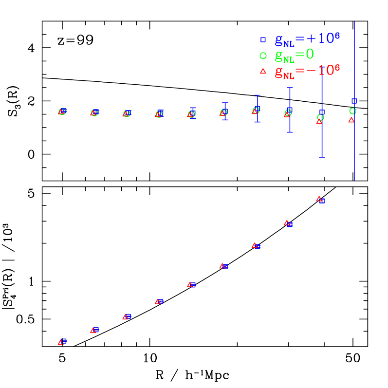
Fig. 1 displays the initial skewness (top panel) and kurtosis (bottom panel) obtained upon distributing the dark matter particles onto a regular 5123 mesh (i.e. of cell size 3h1Mpcabsent3superscript1Mpc\approx 3\ {\rm{\it h}^{-1}Mpc}) using the cloud-in-cell (CIC) interpolation scheme. Symbols represent the numerical results averaged over the realisations. Because S4Zelsuperscriptsubscript𝑆4ZelS_{4}^{\rm Zel} (which is the sole contribution to the kurtosis in the Gaussian case) varies considerably between the realisations, we only show the absolute difference |S4Pri|superscriptsubscript𝑆4Pri|S_{4}^{\rm Pri}| between the kurtosis in the non-Gaussian (gNL=±106subscript𝑔NLplus-or-minussuperscript106g_{\rm NL}=\pm 10^{6}) and the Gaussian (gNL=0subscript𝑔NL0g_{\rm NL}=0) runs. As expected, the skewness is very similar among the Gaussian and non-Gaussian simulations. While S3subscript𝑆3S_{3} in the simulations agrees well with the skewness induced by the Zel’dovich dynamics Eq. (3) (solid curve), it is gradually suppressed as the filtering radius R𝑅R approaches the cell size, presumably because of the finite resolution which smoothes also the fluctuations. Note that, in the simulations with nonzero gNLsubscript𝑔NLg_{\rm NL} and fNLsubscript𝑓NLf_{\rm NL}, there is a large primordial skewness which is of magnitude |S3Pri|similar-tosuperscriptsubscript𝑆3Priabsent|S_{3}^{\rm Pri}|\sim a few on scale R50h1Mpcless-than-or-similar-to𝑅50superscript1MpcR\lesssim 50\ {\rm{\it h}^{-1}Mpc}, consistent with theory. As can also be seen, the absolute value of the primordial kurtosis increases sharply with R𝑅R, in very good agreement with the theoretical prediction.
Refer to caption
Figure 1: Skewness and kurtosis of the initial (z=99𝑧99z=99) density field as a function of smoothing radius. While the top panel shows the sum of the contributions arising from the Zel’dovich dynamics and from primordial non-Gaussianity, S3=S3Zel+S3Prisubscript𝑆3superscriptsubscript𝑆3Zelsuperscriptsubscript𝑆3PriS_{3}=S_{3}^{\rm Zel}+S_{3}^{\rm Pri}, the bottom panel only shows the absolute value of the primordial kurtosis, |S4Pri|superscriptsubscript𝑆4Pri|S_{4}^{\rm Pri}|. Symbols represent the numerical results averaged over the realisations. They have been slightly shifted horizontally for clarity. Error bars show the scatter among the realisations for the models with gNL=106subscript𝑔NLsuperscript106g_{\rm NL}=10^{6}. Solid lines indicate the theoretical expectations.

II.3 The matter power spectrum

Non-Gaussian corrections to the primordial curvature perturbation can renormalise the input power spectrum of fluctuations used to seed the simulations. Since our simulations implement its unrenormalised version Δϕ2(k)=Aϕ(k/k0)ns1superscriptsubscriptΔitalic-ϕ2𝑘subscript𝐴italic-ϕsuperscript𝑘subscript𝑘0subscript𝑛𝑠1\Delta_{\phi}^{2}(k)=A_{\phi}(k/k_{0})^{n_{s}-1}, it is desirable to ascertain the effect of the local coupling term on the simulated density power spectrum before discussing the halo mass function and bias. For fNLsubscript𝑓NLf_{\rm NL} models with |fNL|100less-than-or-similar-tosubscript𝑓NL100|f_{\rm NL}|\lesssim 100, renormalisation effects are unlikely to be noticeable due to the limited dynamical range of current cosmological simulations 2008PhRvD..78l3519M . As we will see shortly however, they can be significant in simulations of gNLsubscript𝑔NLg_{\rm NL} models with similar level of non-Gaussianity.

The cubic order term gNLϕ3subscript𝑔NLsuperscriptitalic-ϕ3g_{\rm NL}\phi^{3} renormalises the amplitude Aϕsubscript𝐴italic-ϕA_{\phi} of the power spectrum of initial curvature perturbations to AϕAϕ+6gNLϕ2subscript𝐴italic-ϕsubscript𝐴italic-ϕ6subscript𝑔NLdelimited-⟨⟩superscriptitalic-ϕ2A_{\phi}\rightarrow A_{\phi}+6g_{\rm NL}\langle\phi^{2}\rangle, where

ϕ2=d3k(2π)3Pϕ(k).delimited-⟨⟩superscriptitalic-ϕ2superscript𝑑3𝑘superscript2𝜋3subscript𝑃italic-ϕ𝑘\langle\phi^{2}\rangle=\int\!\!\frac{d^{3}k}{(2\pi)^{3}}P_{\phi}(k)\;. (7)

For scale invariant initial conditions, ϕ2delimited-⟨⟩superscriptitalic-ϕ2\langle\phi^{2}\rangle has a logarithmic divergence at large and small scales (see 2008PhRvD..78l3519M for a more detailed discussion of perturbative corrections in non-Gaussian cosmologies). In practice, a low- and high-k𝑘k cutoff are naturally provided by the finite box size and the resolution of the simulations. Therefore, the effective amplitude of density fluctuations in non-Gaussian simulations with cubic coupling is σ8+δσ8subscript𝜎8𝛿subscript𝜎8\sigma_{8}+\delta\sigma_{8} with

δσ8𝛿subscript𝜎8\displaystyle\delta\sigma_{8} =3gNLϕ2absent3subscript𝑔NLdelimited-⟨⟩superscriptitalic-ϕ2\displaystyle=3g_{\rm NL}\langle\phi^{2}\rangle (8)
=3gNL(k0kmin)1ns[1(kminkmax)1ns]Aϕ1ns.absent3subscript𝑔NLsuperscriptsubscript𝑘0subscript𝑘min1subscript𝑛𝑠delimited-[]1superscriptsubscript𝑘minsubscript𝑘max1subscript𝑛𝑠subscript𝐴italic-ϕ1subscript𝑛𝑠\displaystyle=3g_{\rm NL}\left(\frac{k_{0}}{k_{\rm min}}\right)^{1-n_{s}}\left[1-\left(\frac{k_{\rm min}}{k_{\rm max}}\right)^{1-n_{s}}\right]\frac{A_{\phi}}{1-n_{s}}\;.

Recall that k0=0.02hMpc1subscript𝑘00.02superscriptMpc1k_{0}=0.02\ {\rm{\it h}Mpc^{-1}} is our choice of normalisation point, and kminsubscript𝑘mink_{\rm min} and kmaxsubscript𝑘maxk_{\rm max} are the integration limits set by the fundamental mode and the Nyquist frequency of the periodic cubical box over which the initial conditions are generated. Equivalently,

δσ8=3gNL(Lk02π)1ns[1Nns1]Aϕ1ns,𝛿subscript𝜎83subscript𝑔NLsuperscript𝐿subscript𝑘02𝜋1subscript𝑛𝑠delimited-[]1superscript𝑁subscript𝑛𝑠1subscript𝐴italic-ϕ1subscript𝑛𝑠\delta\sigma_{8}=3g_{\rm NL}\left(\frac{Lk_{0}}{2\pi}\right)^{1-n_{s}}\left[1-N^{n_{s}-1}\right]\frac{A_{\phi}}{1-n_{s}}\;, (9)

where N=1024𝑁1024N=1024 is the number of mesh points along one dimension. This result becomes δσ8=3gNLln(N)Aϕ𝛿subscript𝜎83subscript𝑔NL𝑁subscript𝐴italic-ϕ\delta\sigma_{8}=3g_{\rm NL}\ln(N)A_{\phi} in the scale-invariant limit ns1subscript𝑛𝑠1n_{s}\rightarrow 1. For the cosmological setup considered here, the absolute deviation is

δσ80.015(gNL106).𝛿subscript𝜎80.015subscript𝑔NLsuperscript106\delta\sigma_{8}\approx 0.015\left(\frac{g_{\rm NL}}{10^{6}}\right)\;. (10)

This correction is fairly large for the values of gNLsubscript𝑔NLg_{\rm NL} adopted here and, therefore, must be taken into account in the comparison between the theory and the simulations. As we will see below, this is especially important when studying the high mass tail of the halo mass function which is exponentially sensitive to the amplitude of density fluctuations.

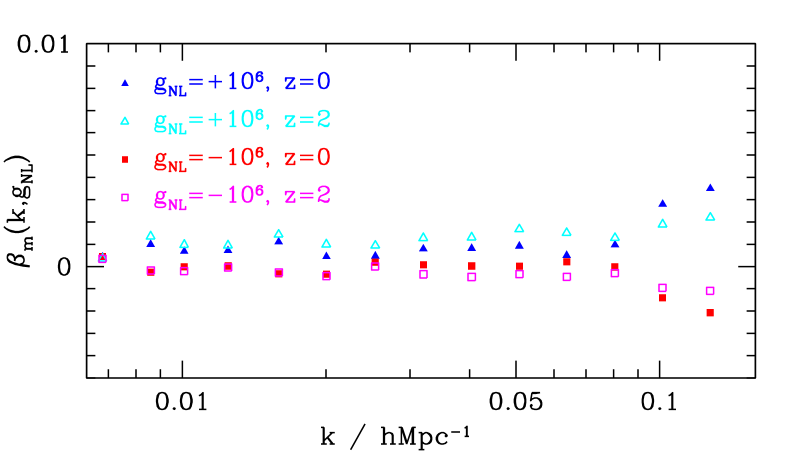
The cubic coupling term gNLϕ3subscript𝑔NLsuperscriptitalic-ϕ3g_{\rm NL}\phi^{3} can also induce a scale-dependent correction to the matter power spectrum which can be quantified by the fractional change βm(k,gNL)=Pmm(k,gNL)/Pmm(k,gNL=0)1subscript𝛽m𝑘subscript𝑔NLsubscript𝑃mm𝑘subscript𝑔NLsubscript𝑃mm𝑘subscript𝑔NL01\beta_{\rm m}(k,g_{\rm NL})=P_{\rm mm}(k,g_{\rm NL})/P_{\rm mm}(k,g_{\rm NL}=0)-1. In Fig. 2, symbols show the result of measuring βm(k,gNL)subscript𝛽m𝑘subscript𝑔NL\beta_{\rm m}(k,g_{\rm NL}) from the snapshots at z=0𝑧0z=0 and 2 after correction of the normalisation shift |2δσ8/σ8|=0.0372𝛿subscript𝜎8subscript𝜎80.037|2\delta\sigma_{8}/\sigma_{8}|=0.037. There is some evidence for a scale-dependent correction at wavenumber k0.1hMpc1greater-than-or-equivalent-to𝑘0.1superscriptMpc1k\gtrsim 0.1\ {\rm{\it h}Mpc^{-1}} but the resulting deviation is broadly consistent with zero. We will thus neglect βm(k,gNL)subscript𝛽m𝑘subscript𝑔NL\beta_{\rm m}(k,g_{\rm NL}) henceforth.

II.4 The halo multiplicity function

Haloes were identified using the MPI parallelised version of the AHF halo finder 2009arXiv0904.3662K which is based on the spherical overdensity (SO) finder developed by 2004MNRAS.351..399G . The main reason for using a SO finder is that it is more closely connected to the predictions of the spherical collapse model, on which most of the analytic formulae presented in this paper are based. Namely, the virial mass M𝑀M of a halo is defined by the radius at which the inner overdensity exceeds Δvir(z)subscriptΔvir𝑧\Delta_{\rm vir}(z) times the background density ρ¯(z)¯𝜌𝑧\bar{\rho}(z) 1992ApJ…399..405W ; 1994MNRAS.271..676L . The value of the overdensity threshold Δvir(z)subscriptΔvir𝑧\Delta_{\rm vir}(z) is obtained from the collapse of a spherical tophat perturbation and has a dependence on redshift through the matter density Ωm(z)subscriptΩ𝑚𝑧\Omega_{m}(z) 1996MNRAS.282..263E ; 1998ApJ…495…80B . We discard poorly resolved haloes and only study those containing at least 34 particles or, equivalently, with a mass larger than M=1013M/h𝑀superscript1013subscriptMdirect-productM=10^{13}\ {\rm M_{\odot}/{\it h}}.

Analytic arguments based on the Press-Schechter theory 1974ApJ…187..425P ; 1991ApJ…379..440B predict that the halo mass function n(M,z)𝑛𝑀𝑧n(M,z) is entirely specified by the distribution νf(ν)𝜈𝑓𝜈\nu f(\nu) of first-crossings, or multiplicity function

νf(ν)=M2n(M,z)ρ¯dlnMdlnν.𝜈𝑓𝜈superscript𝑀2𝑛𝑀𝑧¯𝜌𝑑𝑀𝑑𝜈\nu f(\nu)=M^{2}\,\frac{n(M,z)}{\bar{\rho}}\frac{d\ln M}{d\ln\nu}\;. (11)

The peak height ν(M,z)=δc(z)/σ(M)𝜈𝑀𝑧subscript𝛿c𝑧𝜎𝑀\nu(M,z)=\delta_{\rm c}(z)/\sigma(M) is the typical amplitude of fluctuations that produce haloes of mass M𝑀M by redshift z𝑧z. Here and henceforth, σ(M)𝜎𝑀\sigma(M) denotes the variance of the density field δMsubscript𝛿𝑀\delta_{M} smoothed on mass scale MR3proportional-to𝑀superscript𝑅3M\propto R^{3} and linearly extrapolated to present epoch, whereas δc(z)1.68D(0)/D(z)subscript𝛿c𝑧1.68𝐷0𝐷𝑧\delta_{\rm c}(z)\approx 1.68D(0)/D(z) is the critical linear overdensity for (spherical) collapse at redshift z𝑧z.

Despite the lack of a compelling theoretical description of the multiplicity function for Gaussian initial conditions, the fractional deviation from Gaussianity can be modelled accurately using the Press-Schechter formalism. In this approach, the halo mass function n(M,z)𝑛𝑀𝑧n(M,z) is related to the probability P(>δc,M)P(>\delta_{\rm c},M) that a region of mass M𝑀M exceeds the critical density for collapse δc(z)subscript𝛿c𝑧\delta_{\rm c}(z) through the relation n(M,z)=2(ρ¯/M)dP/dM𝑛𝑀𝑧2¯𝜌𝑀𝑑𝑃𝑑𝑀n(M,z)=-2\,(\bar{\rho}/M)\,dP/dM. The non-Gaussian fractional correction to the multiplicity function then is R(ν,gNL)f(ν,gNL)/f(ν,0)=(dP/dM)(>δc,M,gNL)/(dP/dM)(>δc,M,0)R(\nu,g_{\rm NL})\equiv f(\nu,g_{\rm NL})/f(\nu,0)=(dP/dM)(>\delta_{\rm c},M,g_{\rm NL})/(dP/dM)(>\delta_{\rm c},M,0). The level excursion probability P(>δc,M,gNL)P(>\delta_{\rm c},M,g_{\rm NL}) can be computed once the probability distribution function (PDF) of the smoothed density field δMsubscript𝛿𝑀\delta_{M}, P(δM)𝑃subscript𝛿𝑀P(\delta_{M}), is known. Here, we will consider the simple extensions proposed by 2008JCAP…04..014L and 2000ApJ…541…10M , in which P(δM)𝑃subscript𝛿𝑀P(\delta_{M}) is generically expressed as the inverse transform of a cumulant generating function. Both extensions have been shown to give reasonable agreement with numerical simulations of non-Gaussian cosmologies 2007MNRAS.382.1261G ; 2009MNRAS.396…85D ; 2009arXiv0902.2013G .
Refer to caption
Figure 2: Non-Gaussian fractional correction βm(k,gNL)=Pmm(k,gNL)/Pmm(k,0)1subscript𝛽m𝑘subscript𝑔NLsubscript𝑃mm𝑘subscript𝑔NLsubscript𝑃mm𝑘01\beta_{\rm m}(k,g_{\rm NL})=P_{\rm mm}(k,g_{\rm NL})/P_{\rm mm}(k,0)-1 to the matter power spectrum after subtracting a scale-independent normalisation shift 6gNLϕ26subscript𝑔NLdelimited-⟨⟩superscriptitalic-ϕ26g_{\rm NL}\langle\phi^{2}\rangle induced by the cubic coupling gNLϕ3subscript𝑔NLsuperscriptitalic-ϕ3g_{\rm NL}\phi^{3}.

In 2008JCAP…04..014L , the saddle-point technique is applied directly to P(δM)𝑃subscript𝛿𝑀P(\delta_{M}). The resulting Edgeworth expansion is then used to obtain P(>δc,M,gNL)P(>\delta_{\rm c},M,g_{\rm NL}). For fNLsubscript𝑓NLf_{\rm NL} non-Gaussianity, reference 2009MNRAS.396…85D found that the resulting non-Gaussian mass function agrees well with the simulations. For gNLsubscript𝑔NLg_{\rm NL} non-Gaussianity, neglecting cumulants other than the kurtosis S4Pri(M)superscriptsubscript𝑆4Pri𝑀S_{4}^{\rm Pri}(M) (Hereafter, we drop the superscript for conciseness) and truncating the series expansion at S4(M)subscript𝑆4𝑀S_{4}(M), the non-Gaussian fractional correction reads

RLV(ν,gNL)subscript𝑅LV𝜈subscript𝑔NL\displaystyle R_{\rm LV}(\nu,g_{\rm NL}) {1+14!σ2S4(ν44ν23)\displaystyle\approx\left\{1+\frac{1}{4!}\,\sigma^{2}S_{4}\left(\nu^{4}-4\nu^{2}-3\right)\right. (12)
14!σ2dS4dlnν(ν23)}exp[ν2δσ8]\displaystyle\qquad\left.-\frac{1}{4!}\sigma^{2}\frac{dS_{4}}{d\ln\nu}\left(\nu^{2}-3\right)\right\}\exp\left[\nu^{2}\delta\sigma_{8}\right]
={1+14!σ2S4(ν46ν2+3)\displaystyle=\left\{1+\frac{1}{4!}\,\sigma^{2}S_{4}\left(\nu^{4}-6\nu^{2}+3\right)\right. (13)
14!d(σ2S4)dlnν(ν23)}exp[ν2δσ8]\displaystyle\qquad\left.-\frac{1}{4!}\,\frac{d(\sigma^{2}S_{4})}{d\ln\nu}\left(\nu^{2}-3\right)\right\}\exp\left[\nu^{2}\delta\sigma_{8}\right]

after integration over regions above δc(z)subscript𝛿c𝑧\delta_{\rm c}(z). Note that we have omitted writing the redshift dependence explicitly. Strictly speaking however, R(ν,gNL)𝑅𝜈subscript𝑔NLR(\nu,g_{\rm NL}) depends distinctly upon the variables M𝑀M (or ν𝜈\nu) and z𝑧z due to the presence of σ2S4(M)superscript𝜎2subscript𝑆4𝑀\sigma^{2}S_{4}(M). Our notation is motivated by the fact that the measured non-Gaussian correction, as plotted in Fig.4, appears to depend mostly on the peak height. The exponential factor in the right-hand side is the correction induced by the renormalisation of the amplitude of linear density fluctuations, Eq. (10). For consistency, we have also used the Press-Schechter multiplicity function to derive this last term although a Sheth-Tormen mass function 1999MNRAS.308..119S may be more appropriate.

In 2000ApJ…541…10M , it is the level excursion probability P(>δc,M)P(>\delta_{\rm c},M) that is calculated within the saddle-point approximation. Including only a cubic coupling gNLϕ3subscript𝑔NLsuperscriptitalic-ϕ3g_{\rm NL}\phi^{3} and truncating the resulting expression at the kurtosis, we find

P(>δc,M,gNL)\displaystyle P(>\delta_{\rm c},M,g_{\rm NL}) (14)
12πσδc(1+3gNLσ2ϕ2S412σ2δc2)absent12𝜋𝜎subscript𝛿c13subscript𝑔NLsuperscript𝜎2delimited-⟨⟩superscriptitalic-ϕ2subscript𝑆412superscript𝜎2superscriptsubscript𝛿c2\displaystyle\quad\approx\frac{1}{\sqrt{2\pi}}\frac{\sigma}{\delta_{\rm c}}\left(1+3g_{\rm NL}\sigma^{2}\langle\phi^{2}\rangle-\frac{S_{4}}{12}\sigma^{2}\delta_{\rm c}^{2}\right)
×exp{δc22σ2[16gNLϕ2S412δc2]}absentsuperscriptsubscript𝛿c22superscript𝜎2delimited-[]16subscript𝑔NLdelimited-⟨⟩superscriptitalic-ϕ2subscript𝑆412superscriptsubscript𝛿c2\displaystyle\qquad\times\exp\left\{-\frac{\delta_{\rm c}^{2}}{2\sigma^{2}}\left[1-6g_{\rm NL}\langle\phi^{2}\rangle-\frac{S_{4}}{12}\,\delta_{\rm c}^{2}\right]\right\}

at first order in gNLsubscript𝑔NLg_{\rm NL}. Note that we have already included the renormalisation of the fluctuation amplitude. For rare events, σ1much-less-than𝜎1\sigma\ll 1 and the first parenthesis in the right-hand side can be neglected. To ensure that the resulting mass function is properly normalised, we follow 2009arXiv0906.1042V and use

νf(ν)=M2n(M,z,gNL)ρ¯dlnMdlnν.subscript𝜈𝑓subscript𝜈superscript𝑀2𝑛𝑀𝑧subscript𝑔NL¯𝜌𝑑𝑀𝑑subscript𝜈\nu_{\star}f(\nu_{\star})=M^{2}\,\frac{n(M,z,g_{\rm NL})}{\bar{\rho}}\frac{d\ln M}{d\ln\nu_{\star}}\;. (15)

for the non-Gaussian mass function, where ν=δ/σsubscript𝜈subscript𝛿𝜎\nu_{\star}=\delta_{\star}/\sigma, δ=δc12δσ8S4δc2/12subscript𝛿subscript𝛿c12𝛿subscript𝜎8subscript𝑆4superscriptsubscript𝛿c212\delta_{\star}=\delta_{\rm c}\sqrt{1-2\delta\sigma_{8}-S_{4}\delta_{\rm c}^{2}/12} 111 In local fNLsubscript𝑓NLf_{\rm NL} models, this formula only involves the skewness S3subscript𝑆3S_{3}. As it is incorrectly quoted in some of the literature on non-Gaussian halo mass functions, let us write down its explicit expression: RMVJ(ν,fNL)=exp[S3δc36σ2][δc26δdS3dlnσ+δδc],subscript𝑅MVJ𝜈subscript𝑓NLsubscript𝑆3superscriptsubscript𝛿c36superscript𝜎2delimited-[]superscriptsubscript𝛿c26subscript𝛿𝑑subscript𝑆3𝑑𝜎subscript𝛿subscript𝛿cR_{\rm MVJ}(\nu,f_{\rm NL})=\exp\left[\frac{S_{3}\delta_{\rm c}^{3}}{6\sigma^{2}}\right]\left[\frac{\delta_{\rm c}^{2}}{6\delta_{\star}}\frac{dS_{3}}{d\ln\sigma}+\frac{\delta_{\star}}{\delta_{\rm c}}\right]\;, or, in terms of the peak height ν=δc/σ𝜈subscript𝛿c𝜎\nu=\delta_{\rm c}/\sigma, RMVJ(ν,fNL)exp[ν36σS3][1ν3σS3ν6d(σS3)dlnν],subscript𝑅MVJ𝜈subscript𝑓NLsuperscript𝜈36𝜎subscript𝑆3delimited-[]1𝜈3𝜎subscript𝑆3𝜈6𝑑𝜎subscript𝑆3𝑑𝜈R_{\rm MVJ}(\nu,f_{\rm NL})\approx\exp\left[\frac{\nu^{3}}{6}\sigma S_{3}\right]\left[1-\frac{\nu}{3}\sigma S_{3}-\frac{\nu}{6}\frac{d(\sigma S_{3})}{d\ln\nu}\right]\;, after expanding δ=1S3δc/3subscript𝛿1subscript𝑆3subscript𝛿c3\delta_{\star}=\sqrt{1-S_{3}\delta_{\rm c}/3} at the first order. and f𝑓f is the same multiplicity function as in the Gaussian case. Taking the derivative of the level excursion probability then gives

(dP/dM)(>δc,M,gNL)(dP/dM)(>δc,M,0)\displaystyle\frac{(dP/dM)(>\delta_{\rm c},M,g_{\rm NL})}{(dP/dM)(>\delta_{\rm c},M,0)} exp[S4δc44!σ2+ν2δσ8]absentsubscript𝑆4superscriptsubscript𝛿c44superscript𝜎2superscript𝜈2𝛿subscript𝜎8\displaystyle\approx\exp\left[\frac{S_{4}\delta_{\rm c}^{4}}{4!\sigma^{2}}+\nu^{2}\delta\sigma_{8}\right] (16)
×(δδc+14!δc3δdS4dlnσ).absentsubscript𝛿subscript𝛿c14superscriptsubscript𝛿c3subscript𝛿𝑑subscript𝑆4𝑑𝜎\displaystyle\quad\times\left(\frac{\delta_{\star}}{\delta_{\rm c}}+\frac{1}{4!}\frac{\delta_{\rm c}^{3}}{\delta_{\star}}\frac{dS_{4}}{d\ln\sigma}\right)\;.

The fractional change in the multiplicity function eventually reads as

RMVJ(ν,gNL)subscript𝑅MVJ𝜈subscript𝑔NL\displaystyle R_{\rm MVJ}(\nu,g_{\rm NL}) exp[ν44!σ2S4+ν2δσ8]absentsuperscript𝜈44superscript𝜎2subscript𝑆4superscript𝜈2𝛿subscript𝜎8\displaystyle\approx\exp\left[\frac{\nu^{4}}{4!}\sigma^{2}S_{4}+\nu^{2}\delta\sigma_{8}\right] (17)
×{1ν28σ2S4ν24!d(σ2S4)dlnν}absent1superscript𝜈28superscript𝜎2subscript𝑆4superscript𝜈24𝑑superscript𝜎2subscript𝑆4𝑑𝜈\displaystyle\quad\times\left\{1-\frac{\nu^{2}}{8}\sigma^{2}S_{4}-\frac{\nu^{2}}{4!}\frac{d(\sigma^{2}S_{4})}{d\ln\nu}\right\}

after expanding δsubscript𝛿\delta_{\star} at the first order and ignoring the shift in the normalisation amplitude, i.e. δ±11S4δc2/24superscriptsubscript𝛿plus-or-minus1minus-or-plus1subscript𝑆4superscriptsubscript𝛿c224\delta_{\star}^{\pm 1}\approx 1\mp S_{4}\delta_{\rm c}^{2}/24. In the limit σ2S41much-less-thansuperscript𝜎2subscript𝑆41\sigma^{2}S_{4}\ll 1 and ν1much-greater-than𝜈1\nu\gg 1, the two theoretical expectations reduce to 1+ν4σ2S4/241superscript𝜈4superscript𝜎2subscript𝑆4241+\nu^{4}\sigma^{2}S_{4}/24. However, they differ in the coefficient of the ν2σ2S4superscript𝜈2superscript𝜎2subscript𝑆4\nu^{2}\sigma^{2}S_{4} term, which is 1/414-1/4 and 1/818-1/8 for the LV and MVJ formula, respectively. Therefore, we shall also consider the approximation

R(ν,gNL)𝑅𝜈subscript𝑔NL\displaystyle R(\nu,g_{\rm NL}) =exp[ν44!σ2S4+ν2δσ8]absentsuperscript𝜈44superscript𝜎2subscript𝑆4superscript𝜈2𝛿subscript𝜎8\displaystyle=\exp\left[\frac{\nu^{4}}{4!}\sigma^{2}S_{4}+\nu^{2}\delta\sigma_{8}\right] (18)
×{1ν24σ2S4ν24!d(σ2S4)dlnν},absent1superscript𝜈24superscript𝜎2subscript𝑆4superscript𝜈24𝑑superscript𝜎2subscript𝑆4𝑑𝜈\displaystyle\quad\times\left\{1-\frac{\nu^{2}}{4}\sigma^{2}S_{4}-\frac{\nu^{2}}{4!}\frac{d(\sigma^{2}S_{4})}{d\ln\nu}\right\}\;,

which is designed to match better the Edgeworth expansion of 2008JCAP…04..014L when the peak height is ν1similar-to𝜈1\nu\sim 1.

Calculating the fractional change in the mass function requires knowledge of the kurtosis S4(M)gNLS4(1)(M)subscript𝑆4𝑀subscript𝑔NLsuperscriptsubscript𝑆41𝑀S_{4}(M)\equiv g_{\rm NL}S_{4}^{(1)}(M) of the smoothed density field δMsubscript𝛿𝑀\delta_{M}, which we compute analytically using the general formula (valid for n3𝑛3n\geq 3)

σ2n2Sn(1)(M)superscript𝜎2𝑛2superscriptsubscript𝑆𝑛1𝑀\displaystyle\sigma^{2n-2}S_{n}^{(1)}(M) =n!(i=1n1d3ki(2π)3αM(ki)Pϕ(ki))absent𝑛superscriptsubscriptproduct𝑖1𝑛1superscript𝑑3subscript𝑘𝑖superscript2𝜋3subscript𝛼𝑀subscript𝑘𝑖subscript𝑃italic-ϕsubscript𝑘𝑖\displaystyle=n!\left(\prod_{i=1}^{n-1}\int\!\!\frac{d^{3}k_{i}}{(2\pi)^{3}}\,\alpha_{M}(k_{i})P_{\phi}(k_{i})\right)
×αM(|𝐤1++𝐤n1|),absentsubscript𝛼𝑀subscript𝐤1subscript𝐤𝑛1\displaystyle\quad\times\alpha_{M}\bigl{(}|{\bf k}_{1}+\cdots+{\bf k}_{n-1}|\bigr{)}\;, (19)

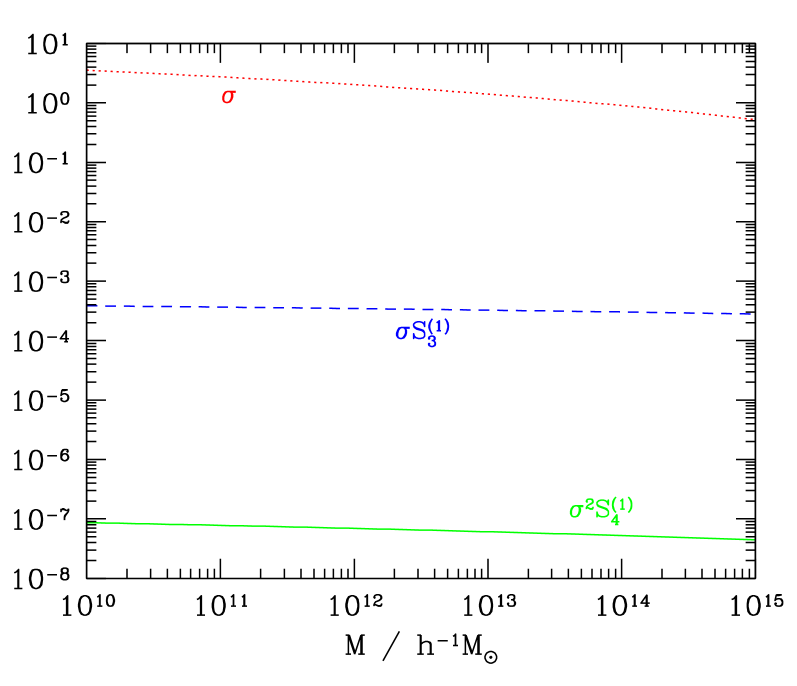
where αM(k)αR(k,z=0)subscript𝛼𝑀𝑘subscript𝛼𝑅𝑘𝑧0\alpha_{M}(k)\equiv\alpha_{R}(k,z=0) in what follows. Over the mass range probed by our simulations, 1013M5×1015M/hless-than-or-similar-tosuperscript1013𝑀less-than-or-similar-to5superscript1015subscriptMdirect-product10^{13}\lesssim M\lesssim 5\times 10^{15}\ {\rm M_{\odot}/{\it h}}, the normalised kurtosis σ2S4(1)(M)superscript𝜎2superscriptsubscript𝑆41𝑀\sigma^{2}S_{4}^{(1)}(M) is a monotonic decreasing function of M𝑀M that varies in the narrow range 46×107similar-toabsent46superscript107\sim 4-6\times 10^{-7} for the top-hat filter assumed here (see Fig. 3). Note also that the σ2S4superscript𝜎2subscript𝑆4\sigma^{2}S_{4} term dominates the total contribution to the non-Gaussian correction eqs. (13), (17) and (18) when the peak height is ν2greater-than-or-equivalent-to𝜈2\nu\gtrsim 2 (One finds |d(σ2S4)/dlnν|0.1σ2S4less-than-or-similar-to𝑑superscript𝜎2subscript𝑆4𝑑𝜈0.1superscript𝜎2subscript𝑆4|d(\sigma^{2}S_{4})/d\ln\nu|\lesssim 0.1\sigma^{2}S_{4}).

Refer to caption
Figure 3: Variance σ𝜎\sigma (dotted), skewness σS3(1)𝜎superscriptsubscript𝑆31\sigma S_{3}^{(1)} (dashed) and kurtosis σ2S4(1)superscript𝜎2superscriptsubscript𝑆41\sigma^{2}S_{4}^{(1)} (solid) of the smoothed linear density field δMsubscript𝛿𝑀\delta_{M} as a function of mass scale M𝑀M.
Refer to caption
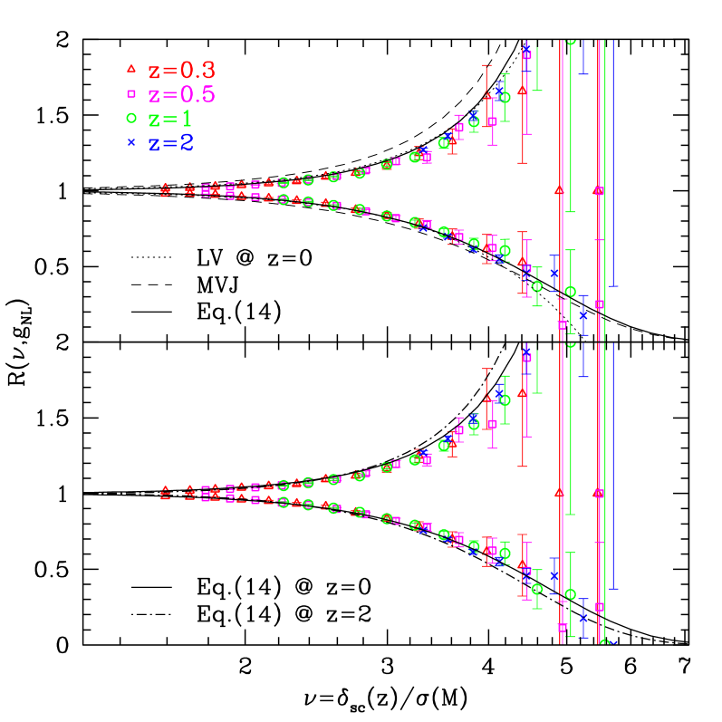
Figure 4: Top panel : Fractional correction to the Gaussian multiplicity function of dark matter haloes as a function of the peak height ν(M,z)𝜈𝑀𝑧\nu(M,z) for a coupling parameter gNL=±106subscript𝑔NLplus-or-minussuperscript106g_{\rm NL}=\pm 10^{6}. The dotted, dashed and solid curves show the theoretical predictions eqs. (13), (17) and (18) at z=0𝑧0z=0, respectively. Error bars denote Poisson errors. For illustration, M=1015M/h𝑀superscript1015subscriptMdirect-productM=10^{15}\ {\rm M_{\odot}/{\it h}} corresponds to ν=3.2𝜈3.2\nu=3.2, 5.2, 7.7 at redshift z=0𝑧0z=0, 1 and 2, respectively. Similarly, M=1014M/h𝑀superscript1014subscriptMdirect-productM=10^{14}\ {\rm M_{\odot}/{\it h}} and 1013M/hsuperscript1013subscriptMdirect-product10^{13}\ {\rm M_{\odot}/{\it h}} correspond to ν=1.9𝜈1.9\nu=1.9, 3, 4.5 and 1.2, 1.9, 2.9 respectively. Bottom panel : a comparison with equation (18) evaluated at z=0𝑧0z=0 and 2.

The fractional correction is plotted in Fig. 4 for the haloes extracted from the simulations at redshift z=0.3𝑧0.3z=0.3, 0.5, 1 and 2. In the top panel, the data are compared to the theoretical predictions eqs. (13), (17) and (18) evaluated at z=0𝑧0z=0. As we can see, the level of non-Gaussianity in the halo multiplicity function is consistent with the theory. Our approximation (18) performs equally well regardless of the sign of gNLsubscript𝑔NLg_{\rm NL}. It agrees better with the measurements than the formulae of 2000ApJ…541…10M which significantly overestimates the data for gNL=106subscript𝑔NLsuperscript106g_{\rm NL}=10^{6}, and than that of 2008JCAP…04..014L which is not always positive definite for gNL=106subscript𝑔NLsuperscript106g_{\rm NL}=-10^{6}. The bottom panel shows that the discrepancy somewhat worsens at higher redshift, especially in the case gNL=106subscript𝑔NLsuperscript106g_{\rm NL}=10^{6}. However, it is possible the agreement may be improved by adding higher order powers of σ2S4superscript𝜎2subscript𝑆4\sigma^{2}S_{4} and higher order cumulants.

To conclude this section, one should keep in mind that all these extensions are based on Press-Schechter and, therefore, provide a bad fit to the Gaussian mass function of haloes. In this respect, excursion set approaches may be more promising since they seem to reproduce both the Gaussian halo counts and the dependence on fNLsubscript𝑓NLf_{\rm NL} 2009arXiv0905.1702L ; 2009MNRAS.399.1482L .

III The non-Gaussian bias shift

III.1 Theoretical considerations

In order to calculate the scale-dependent bias correction induced by the gNLsubscript𝑔NLg_{\rm NL} coupling term to the correlation of haloes of mass M𝑀M collapsing at redshift z𝑧z, we follow 2008ApJ…677L..77M and consider the two-point correlation ξhh(𝐫)subscript𝜉hh𝐫\xi_{\rm hh}({\bf r}) of regions of the smoothed density field δMsubscript𝛿𝑀\delta_{M} above a threshold δc(z)=ν(z)σsubscript𝛿𝑐𝑧𝜈𝑧𝜎\delta_{c}(z)=\nu(z)\sigma. The two-point correlation function of this level excursion set, which was originally derived by 1986ApJ…310L..21M , can be expressed in the high threshold approximation as

ξhh(𝐫)subscript𝜉hh𝐫\displaystyle\xi_{\rm hh}({\bf r}) =1+exp{n=2j=1n1νnσnj!(nj)!\displaystyle=-1+\exp\left\{\sum_{n=2}^{\infty}\sum_{j=1}^{n-1}\frac{\nu^{n}\sigma^{-n}}{j!(n-j)!}\right. (20)
×ξ(n)(𝐱1,,𝐱1,𝐱2,,𝐱2jtimes(nj)times)},\displaystyle\qquad\left.\times\xi^{(n)}\!\left(\begin{array}[]{cc}{\bf x}_{1},\cdots,{\bf x}_{1},&{\bf x}_{2},\cdots,{\bf x}_{2}\\ j~{}\mbox{times}&(n-j)~{}\mbox{times}\end{array}\right)\right\}\;, (23)

where 𝐫=𝐱1𝐱2𝐫subscript𝐱1subscript𝐱2{\bf r}={\bf x}_{1}-{\bf x}_{2}. For the non-Gaussian model considered here, the leading-order correction induced by non-zero three-point and four-point correlations of the density field reads

ΔξhhΔsubscript𝜉hh\displaystyle\Delta\xi_{\rm hh} =ν3σ3ξ(3)(𝐱1,𝐱1,𝐱2)+ν4σ4[13ξ(4)(𝐱1,𝐱1,𝐱1,𝐱2)\displaystyle=\frac{\nu^{3}}{\sigma^{3}}\xi^{(3)}({\bf x}_{1},{\bf x}_{1},{\bf x}_{2})+\frac{\nu^{4}}{\sigma^{4}}\left[\frac{1}{3}\xi^{(4)}({\bf x}_{1},{\bf x}_{1},{\bf x}_{1},{\bf x}_{2})\right.
+14ξ(4)(𝐱1,𝐱1,𝐱2,𝐱2)].\displaystyle\qquad\left.+\frac{1}{4}\xi^{(4)}({\bf x}_{1},{\bf x}_{1},{\bf x}_{2},{\bf x}_{2})\right]\;. (24)

The non-Gaussian correction ΔPhhΔsubscript𝑃hh\Delta P_{\rm hh} to the power spectrum of biased tracers is obtained by Fourier transforming this expression.

In the case fNL=0subscript𝑓NL0f_{\rm NL}=0 and gNL0subscript𝑔NL0g_{\rm NL}\neq 0, only the four-point functions contribute at first order. It should also be noted that, at linear order, ξ(2)(𝐱1,𝐱2)superscript𝜉2subscript𝐱1subscript𝐱2\xi^{(2)}({\bf x}_{1},{\bf x}_{2}) amounts to a renormalisation of the linear bias and, therefore, does not contribute to the scale-dependent correction. Details of the calculation can be found in Appendix A. In short, the non-Gaussian correction ΔPhhΔsubscript𝑃hh\Delta P_{\rm hh} in the limit of long wavelength k1much-less-than𝑘1k\ll 1 is given by the Fourier transform of ν4ξ(4)(𝐱1,𝐱1,𝐱2,𝐱2)/3σ4superscript𝜈4superscript𝜉4subscript𝐱1subscript𝐱1subscript𝐱2subscript𝐱23superscript𝜎4\nu^{4}\xi^{(4)}({\bf x}_{1},{\bf x}_{1},{\bf x}_{2},{\bf x}_{2})/3\sigma^{4},

ΔPhh(k)Δsubscript𝑃hh𝑘\displaystyle\Delta P_{\rm hh}(k) =gNLν4S3(1)(M)αM(k)Pϕ(k)absentsubscript𝑔NLsuperscript𝜈4superscriptsubscript𝑆31𝑀subscript𝛼𝑀𝑘subscript𝑃italic-ϕ𝑘\displaystyle=g_{\rm NL}\nu^{4}\,S_{3}^{(1)}\!(M)\alpha_{M}(k)P_{\phi}(k) (25)
=gNLbL2(z)δc2(z)S3(1)(M)αM(k)Pϕ(k),absentsubscript𝑔NLsuperscriptsubscript𝑏L2𝑧superscriptsubscript𝛿𝑐2𝑧superscriptsubscript𝑆31𝑀subscript𝛼𝑀𝑘subscript𝑃italic-ϕ𝑘\displaystyle=g_{\rm NL}b_{\rm L}^{2}(z)\delta_{c}^{2}(z)\,S_{3}^{(1)}\!(M)\alpha_{M}(k)P_{\phi}(k)\;,

where we have used bL(z)=ν2/δc(z)subscript𝑏L𝑧superscript𝜈2subscript𝛿𝑐𝑧b_{\rm L}(z)=\nu^{2}/\delta_{c}(z) as is appropriate for high density peaks. The smoothing window that appears in αM(k)subscript𝛼𝑀𝑘\alpha_{M}(k) effectively makes little difference because we are considering the limit where k1superscript𝑘1k^{-1} is much larger than the smoothing radius, so we will omit it in the following. For small non-Gaussianity, we can also write ΔPhh2bLΔbκPδ(k)Δsubscript𝑃hh2subscript𝑏LΔsubscript𝑏𝜅subscript𝑃𝛿𝑘\Delta P_{\rm hh}\approx 2b_{\rm L}\Delta b_{\kappa}P_{\delta}(k) where Pδ(k)=αM2Pϕ(k)subscript𝑃𝛿𝑘superscriptsubscript𝛼𝑀2subscript𝑃italic-ϕ𝑘P_{\delta}(k)=\alpha_{M}^{2}P_{\phi}(k) is the power spectrum of the smoothed density field. The scale-dependent bias correction Δbκ(k,gNL)Δsubscript𝑏𝜅𝑘subscript𝑔NL\Delta b_{\kappa}(k,g_{\rm NL}) can eventually be recast into the form

Δbκ(k,gNL)Δsubscript𝑏𝜅𝑘subscript𝑔NL\displaystyle\Delta b_{\kappa}(k,g_{\rm NL}) =12gNLbL(z)δc2(z)S3(1)(M)αM1(k)absent12subscript𝑔NLsubscript𝑏L𝑧superscriptsubscript𝛿𝑐2𝑧superscriptsubscript𝑆31𝑀superscriptsubscript𝛼𝑀1𝑘\displaystyle=\frac{1}{2}g_{\rm NL}b_{\rm L}(z)\delta_{c}^{2}(z)\,S_{3}^{(1)}\!(M)\alpha_{M}^{-1}(k) (26)
=34gNLbL(z)δc2(0)D(0)D(z)2S3(1)(M)ΩmH02k2T(k)absent34subscript𝑔NLsubscript𝑏L𝑧superscriptsubscript𝛿𝑐20𝐷0𝐷superscript𝑧2superscriptsubscript𝑆31𝑀subscriptΩmsuperscriptsubscript𝐻02superscript𝑘2𝑇𝑘\displaystyle=\frac{3}{4}g_{\rm NL}b_{\rm L}(z)\delta_{c}^{2}(0)\frac{D(0)}{D(z)^{2}}\,S_{3}^{(1)}\!(M)\frac{\Omega_{\rm m}H_{0}^{2}}{k^{2}T(k)}
=14gNLδc(z)S3(1)(M)Δbκ(k,fNL=1),absent14subscript𝑔NLsubscript𝛿𝑐𝑧superscriptsubscript𝑆31𝑀Δsubscript𝑏𝜅𝑘subscript𝑓NL1\displaystyle=\frac{1}{4}g_{\rm NL}\delta_{c}(z)\,S_{3}^{(1)}\!(M)\,\Delta b_{\kappa}(k,f_{\rm NL}=1)\;,

where Δbκ(k,fNL)Δsubscript𝑏𝜅𝑘subscript𝑓NL\Delta b_{\kappa}(k,f_{\rm NL}) is the scale-independent bias induced by the quadratic coupling fNLϕ2subscript𝑓NLsuperscriptitalic-ϕ2f_{\rm NL}\phi^{2}, Eq. (2). We have also assumed the Eulerian bias prescription b(M)=1+bL(M)𝑏𝑀1subscript𝑏L𝑀b(M)=1+b_{\rm L}(M).

Refer to caption
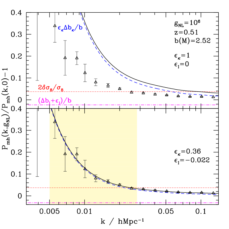
Figure 5: Top panel : Non-Gaussian bias correction computed from the halo-matter power spectrum of haloes of mass M>2×10¹³M/h𝑀2superscript1013subscriptMdirect-productM>2\times 10^{13}\ {\rm M_{\odot}/{\it h}} extracted from the snapshot at z=0.5𝑧0.5z=0.5 (filled symbols). The solid curve represents Pmh(k,gNL)/Pmh(k,0)1subscript𝑃mh𝑘subscript𝑔NLsubscript𝑃mh𝑘01P_{\rm mh}(k,g_{\rm NL})/P_{\rm mh}(k,0)-1 with a non-Gaussian bias shift Δb(k,gNL)Δ𝑏𝑘subscript𝑔NL\Delta b(k,g_{\rm NL}) given by Eq. (29). The dashed, dotted and dotted-dashed curves show three separate contributions that arise at first order in gNLsubscript𝑔NLg_{\rm NL}. Bottom panel : Δb(k,gNL)Δ𝑏𝑘subscript𝑔NL\Delta b(k,g_{\rm NL}) is replaced by the theoretical model Eq. (30). The shaded region indicates the data points used to fit the parameters ϵκsubscriptitalic-ϵ𝜅\epsilon_{\kappa} and ϵIsubscriptitalic-ϵI\epsilon_{\rm I}. Error bars indicate the scatter among 5 realisations.

The change in the mean number density of haloes also creates a scale-independent shift which we denote by ΔbI(gNL)Δsubscript𝑏Isubscript𝑔NL\Delta b_{\rm I}(g_{\rm NL}). As shown in 2009MNRAS.396…85D for fNLsubscript𝑓NLf_{\rm NL} models, the inclusion of this correction noticeably improves the agreement with the simulations at wavenumber k0.1hMpc1less-than-or-similar-to𝑘0.1superscriptMpc1k\lesssim 0.1\ {\rm{\it h}Mpc^{-1}}. Using a peak-background split and considering the limit of small non-Gaussianity, this contribution reads

ΔbI(gNL)Δsubscript𝑏Isubscript𝑔NL\displaystyle\Delta b_{\rm I}(g_{\rm NL}) =1σνln[R(ν,gNL)]absent1𝜎𝜈𝑅𝜈subscript𝑔NL\displaystyle=-\frac{1}{\sigma}\frac{\partial}{\partial\nu}\ln\bigl{[}R(\nu,g_{\rm NL})\bigr{]}
1σ[13!(ν33ν)σ2S4+2νδσ8\displaystyle\approx-\frac{1}{\sigma}\left[\frac{1}{3!}\left(\nu^{3}-3\nu\right)\sigma^{2}S_{4}+2\nu\delta\sigma_{8}\right. (27)
+14!(ν38ν)d(σ2S4)dlnνν4!d2(σ2S4)dlnν2]\displaystyle\qquad\left.+\frac{1}{4!}\left(\nu^{3}-8\nu\right)\frac{d(\sigma^{2}S_{4})}{d\ln\nu}-\frac{\nu}{4!}\frac{d^{2}(\sigma^{2}S_{4})}{d\ln\nu^{2}}\right]

after truncating ΔbIΔsubscript𝑏I\Delta b_{\rm I} at first order in gNLsubscript𝑔NLg_{\rm NL} This approximation should perform reasonably well for moderate values of the peak height, ν4less-than-or-similar-to𝜈4\nu\lesssim 4, for which the fractional change in the mass function, equation (18), matches well the numerical data. It is worth noticing that ΔbI(gNL)Δsubscript𝑏Isubscript𝑔NL\Delta b_{\rm I}(g_{\rm NL}) has a sign opposite to that of gNLsubscript𝑔NLg_{\rm NL} because the bias decreases when the mass function goes up. ΔbI(gNL)Δsubscript𝑏Isubscript𝑔NL\Delta b_{\rm I}(g_{\rm NL}) also includes a correction induced by the renormalisation of σ8subscript𝜎8\sigma_{8}. In practice, we estimate ΔbI(gNL)Δsubscript𝑏Isubscript𝑔NL\Delta b_{\rm I}(g_{\rm NL}) for a given halo sample by evaluating σ2S4superscript𝜎2subscript𝑆4\sigma^{2}S_{4} and ν𝜈\nu at the scale corresponding to the average halo mass M¯¯𝑀\bar{M} of the sample, as it is unclear to which extent R(ν,gNL)𝑅𝜈subscript𝑔NLR(\nu,g_{\rm NL}) agrees with the data in the limit MMmuch-greater-than𝑀subscript𝑀M\gg M_{\star}.

III.2 Comparison with the simulations

To assess the effect of primordial non-Gaussianity on the halo bias, we will consider the ratios

Pmh(k,gNL)Pmh(k,0)1subscript𝑃mh𝑘subscript𝑔NLsubscript𝑃mh𝑘01\displaystyle\frac{P_{\rm mh}(k,g_{\rm NL})}{P_{\rm mh}(k,0)}-1 =Δb(k,gNL)b(M)+2δσ8σ8absentΔ𝑏𝑘subscript𝑔NL𝑏𝑀2𝛿subscript𝜎8subscript𝜎8\displaystyle=\frac{\Delta b(k,g_{\rm NL})}{b(M)}+2\frac{\delta\sigma_{8}}{\sigma_{8}} (28)
Phh(k,gNL)Phh(k,0)1subscript𝑃hh𝑘subscript𝑔NLsubscript𝑃hh𝑘01\displaystyle\frac{P_{\rm hh}(k,g_{\rm NL})}{P_{\rm hh}(k,0)}-1 =(1+Δb(k,gNL)b(M))2+2δσ8σ81,absentsuperscript1Δ𝑏𝑘subscript𝑔NL𝑏𝑀22𝛿subscript𝜎8subscript𝜎81\displaystyle=\left(1+\frac{\Delta b(k,g_{\rm NL})}{b(M)}\right)^{2}+2\frac{\delta\sigma_{8}}{\sigma_{8}}-1\;,

where Δb(k,gNL)Δ𝑏𝑘subscript𝑔NL\Delta b(k,g_{\rm NL}) is generally the sum of a scale-dependent and a scale-independent term. One should bear in mind that the scale-independent shift 2δσ8/σ82𝛿subscript𝜎8subscript𝜎82\delta\sigma_{8}/\sigma_{8} arises from the matter power spectrum and, therefore, is distinct from the term 2νδσ8/σ2𝜈𝛿subscript𝜎8𝜎-2\nu\delta\sigma_{8}/\sigma appearing in ΔbIΔsubscript𝑏I\Delta b_{\rm I}. Following 2009MNRAS.396…85D , we shall also quantify the departure from the theoretical scaling as a function of wavemode amplitude with the ratio Δbs/ΔbtΔsuperscript𝑏𝑠Δsuperscript𝑏𝑡\Delta b^{s}/\Delta b^{t}, where ΔbsΔsuperscript𝑏𝑠\Delta b^{s} is the non-Gaussian bias correction measured from the simulation and ΔbtΔsuperscript𝑏𝑡\Delta b^{t} is Eq. (30).

We interpolate the dark matter particles and halo centres onto a regular cubical mesh. The resulting dark matter and halo fluctuation fields are then Fourier transformed to yield the matter-matter, halo-matter and halo-halo power spectra Pmm(k)subscript𝑃mm𝑘P_{\rm mm}(k), Pmh(k)subscript𝑃mh𝑘P_{\rm mh}(k) and Phh(k)subscript𝑃hh𝑘P_{\rm hh}(k), respectively. These power spectra are measured for a range of halo masses and redshifts, covering the relevant range of statistical properties corresponding to the available data sets of galaxy or quasar populations with different luminosities and bias. Note that these quantities are computed on a 5123 grid, whose Nyquist wavenumber is sufficiently large (1hMpc1absent1superscriptMpc1\approx 1\ {\rm{\it h}Mpc^{-1}}) to allow for an accurate measurement of the power in wavemodes of amplitude k0.1hMpc1less-than-or-similar-to𝑘0.1superscriptMpc1k\lesssim 0.1\ {\rm{\it h}Mpc^{-1}}. The halo power spectrum is corrected for the shot-noise due to the discrete nature of dark matter haloes, which we assume to be the standard Poisson term 1/n¯h1subscript¯𝑛h1/\bar{n}_{\rm h}. This discreteness correction is negligible for Pmm(k)subscript𝑃mm𝑘P_{\rm mm}(k) due to the large number of dark matter particles. Yet another important quantity is the linear halo bias b(M)𝑏𝑀b(M) which must be measured accurately from the Gaussian simulations as it controls the magnitude of the scale-dependent shift. Here, we shall use the ratio Pmh(k)/Pmm(k)subscript𝑃mh𝑘subscript𝑃mm𝑘P_{\rm mh}(k)/P_{\rm mm}(k) as a proxy for the halo bias since it is less sensitive to shot-noise.
Refer to caption
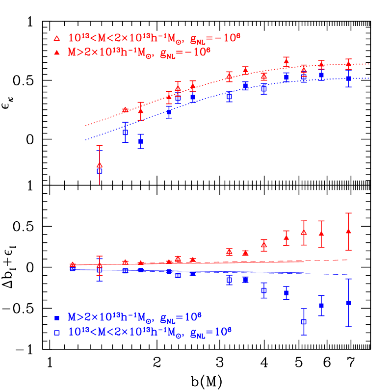
Figure 6: Best-fitting ϵκsubscriptitalic-ϵ𝜅\epsilon_{\kappa} and ΔbI+ϵIΔsubscript𝑏Isubscriptitalic-ϵI\Delta b_{\rm I}+\epsilon_{\rm I} as a function of halo bias and gNL=±106subscript𝑔NLplus-or-minussuperscript106g_{\rm NL}=\pm 10^{6}, for two different mass cuts as indicated in the Figure. In the top panel, the dotted curve is our best fit to ϵκ(b,gNL)subscriptitalic-ϵ𝜅𝑏subscript𝑔NL\epsilon_{\kappa}(b,g_{\rm NL}). In the bottom panel, the solid and dashed lines show the scale-independent shift ΔbIΔsubscript𝑏I\Delta b_{\rm I} predicted by a peak-background split, Eq. (III.1), for the low and high mass samples, respectively.
Refer to caption
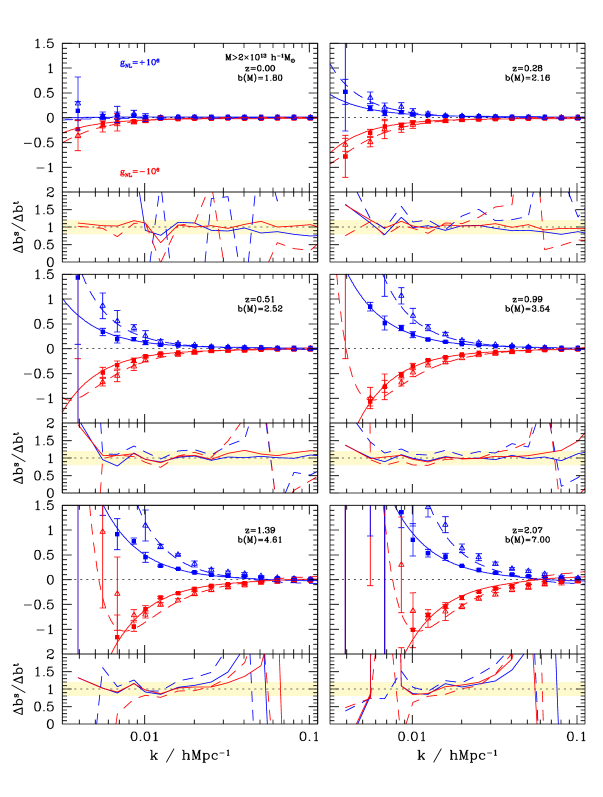
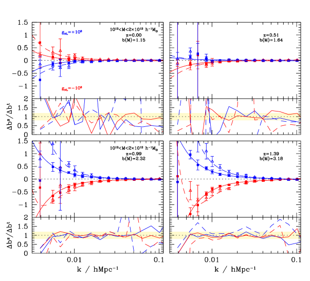
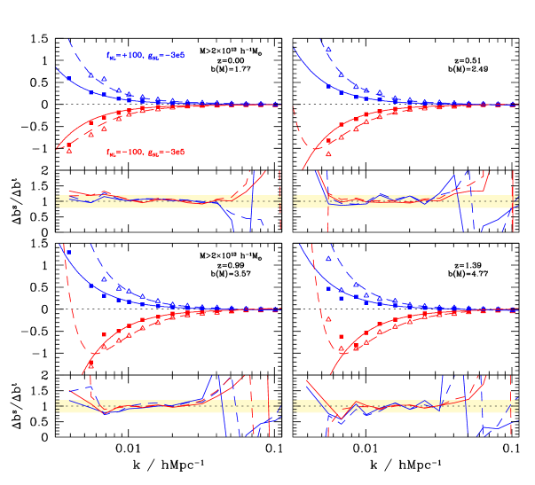
Figure 7: Non-Gaussian bias correction measured in the simulation outputs at redshift 0<z<20𝑧20<z<2 for haloes of mass M>2×10¹³M/h𝑀2superscript1013subscriptMdirect-productM>2\times 10^{13}\ {\rm M_{\odot}/{\it h}}. In each panel, the upper plot shows the ratio Phh(k,gNL)/Phh(k,0)1subscript𝑃hh𝑘subscript𝑔NLsubscript𝑃hh𝑘01P_{\rm hh}(k,g_{\rm NL})/P_{\rm hh}(k,0)-1 (dashed curves, empty symbols) and Pmh(k,gNL)/Pmh(k,0)1subscript𝑃mh𝑘subscript𝑔NLsubscript𝑃mh𝑘01P_{\rm mh}(k,g_{\rm NL})/P_{\rm mh}(k,0)-1 (solid curves, filled symbols). The error bars represent the scatter among 5 realisations. The respective output redshift and linear halo bias are also quoted. The bottom of each panel displays the departure from the theoretical prediction, Δbs/ΔbtΔsuperscript𝑏𝑠Δsuperscript𝑏𝑡\Delta b^{s}/\Delta b^{t}. The shaded area indicates the domain where the deviation is less than 20 per cent. The parameters ϵκsubscriptitalic-ϵ𝜅\epsilon_{\kappa} and ϵIsubscriptitalic-ϵI\epsilon_{\rm I} are fitted individually to each sample. For illustration, ϵκsubscriptitalic-ϵ𝜅\epsilon_{\kappa} takes the best-fit values 0.06 and 0.60 for the lowest and highest biased samples, respectively.
Refer to caption
Figure 8: Same as Fig. 7 but for haloes in the mass range 1013<M<2×10¹³M/hsuperscript1013𝑀2superscript1013subscriptMdirect-product10^{13}<M<2\times 10^{13}\ {\rm M_{\odot}/{\it h}}.

III.2.1 An effective non-Gaussian bias correction

Summarizing the analytical considerations of Sec. III.1, non-Gaussianity of the gNLsubscript𝑔NLg_{\rm NL} type add a correction Δb(k,gNL)Δ𝑏𝑘subscript𝑔NL\Delta b(k,g_{\rm NL}) to the bias b(k)𝑏𝑘b(k) of dark matter haloes which is at leading order

Δb(k,gNL)=Δbκ(k,gNL)+ΔbI(gNL),Δ𝑏𝑘subscript𝑔NLΔsubscript𝑏𝜅𝑘subscript𝑔NLΔsubscript𝑏Isubscript𝑔NL\Delta b(k,g_{\rm NL})=\Delta b_{\kappa}(k,g_{\rm NL})+\Delta b_{\rm I}(g_{\rm NL})\;, (29)

We found, however, that this theoretical expectation significantly overestimates the magnitude of the non-Gaussian bias shift measured from the simulations. This is exemplified in the top panel of Fig. 5, where Pmh(k,gNL)/Pmh(k,0)1subscript𝑃mh𝑘subscript𝑔NLsubscript𝑃mh𝑘01P_{\rm mh}(k,g_{\rm NL})/P_{\rm mh}(k,0)-1 is plotted for haloes of mass M>2×10¹³M/h𝑀2superscript1013subscriptMdirect-productM>2\times 10^{13}\ {\rm M_{\odot}/{\it h}} identified at z=0.5𝑧0.5z=0.5. Clearly, the predicted scale-dependent correction ΔbκΔsubscript𝑏𝜅\Delta b_{\kappa} is much steeper than measured from the halo samples. In order to improve the agreement with the numerical data, we modify the above relation as follows :

Δb(k,gNL)=ϵκΔbκ(k,gNL)+[ΔbI(gNL)+ϵI],Δ𝑏𝑘subscript𝑔NLsubscriptitalic-ϵ𝜅Δsubscript𝑏𝜅𝑘subscript𝑔NLdelimited-[]Δsubscript𝑏Isubscript𝑔NLsubscriptitalic-ϵI\Delta b(k,g_{\rm NL})=\epsilon_{\kappa}\,\Delta b_{\kappa}(k,g_{\rm NL})+\bigl{[}\Delta b_{\rm I}(g_{\rm NL})+\epsilon_{\rm I}\bigr{]}\;, (30)

and treat ϵκsubscriptitalic-ϵ𝜅\epsilon_{\kappa} and ϵIsubscriptitalic-ϵI\epsilon_{\rm I} as free parameters that we fit to our measurements of the cross-power spectrum (weighted by the scatter among 5 realisations) in the range 0.005k0.03hMpc10.005𝑘0.03superscriptMpc10.005\leq k\leq 0.03\ {\rm{\it h}Mpc^{-1}} where the scale-dependent effect is largest. The bottom panel of Fig. 5 shows the resulting best-fit contributions ϵκΔbκsubscriptitalic-ϵ𝜅Δsubscript𝑏𝜅\epsilon_{\kappa}\Delta b_{\kappa} and ΔbI+ϵIΔsubscript𝑏Isubscriptitalic-ϵI\Delta b_{\rm I}+\epsilon_{\rm I} for the halo sample mentioned above. As seen in Fig. 6, ϵκsubscriptitalic-ϵ𝜅\epsilon_{\kappa} and ϵIsubscriptitalic-ϵI\epsilon_{\rm I} appear to depend mainly upon the linear halo bias b(M)𝑏𝑀b(M) and the coupling parameter gNLsubscript𝑔NLg_{\rm NL}, although dependencies on redshift or other halo observables are not excluded (The data is too noisy for a reliable estimate of these). The most striking feature of Fig. 6 is the functional dependence of ϵκsubscriptitalic-ϵ𝜅\epsilon_{\kappa} on b(M)𝑏𝑀b(M) and gNLsubscript𝑔NLg_{\rm NL}. Firstly, ϵκsubscriptitalic-ϵ𝜅\epsilon_{\kappa} is a monotonically increasing function of the bias and never reaches unity, even for the most biased samples for which the high peak approximation should be valid. Secondly, ϵκsubscriptitalic-ϵ𝜅\epsilon_{\kappa} is noticeably larger for gNL=106subscript𝑔NLsuperscript106g_{\rm NL}=-10^{6}, suggesting thereby that second (and higher) order contributions to the scale-dependent bias may be important. Furthermore, for b1.5less-than-or-similar-to𝑏1.5b\lesssim 1.5 where the high peak approximation breaks down, there is some evidence that the effect reverses sign. The bottom panel of Fig. 6 shows that the scale-independent correction has sign opposite to that of gNLsubscript𝑔NLg_{\rm NL}, in agreement with theoretical expectations from the peak-background split (see Sec.III.1). However, whereas for b3less-than-or-similar-to𝑏3b\lesssim 3 the magnitude of the correction is comparable to that predicted by Eq. (III.1), it is considerably larger for b3greater-than-or-equivalent-to𝑏3b\gtrsim 3, reaching up to 5-10 per cent of the linear halo bias.

Assuming ϵκsubscriptitalic-ϵ𝜅\epsilon_{\kappa} is a function of b(M)𝑏𝑀b(M) and gNLsubscript𝑔NLg_{\rm NL} only and asymptotes to a constant in the highly biased limit, we find that the following parametrised form

ϵκ(b,gNL)=c1c2gNLc31+exp(c4b)subscriptitalic-ϵ𝜅𝑏subscript𝑔NLsubscript𝑐1subscript𝑐2subscript𝑔NLsubscript𝑐31subscript𝑐4𝑏\epsilon_{\kappa}(b,g_{\rm NL})=c_{1}-c_{2}\,g_{\rm NL}-\frac{c_{3}}{1+\exp(c_{4}b)} (31)

captures reasonably well the increase of ϵκsubscriptitalic-ϵ𝜅\epsilon_{\kappa} with halo bias for 1.5<b(M)<71.5𝑏𝑀71.5<b(M)<7. The best-fit values of the parameters are

c1=0.59±0.03,c2=(6.0±0.9)×108formulae-sequencesubscript𝑐1plus-or-minus0.590.03subscript𝑐2plus-or-minus6.00.9superscript108\displaystyle c_{1}=0.59\pm 0.03,\quad c_{2}=(6.0\pm 0.9)\times 10^{-8} (32)
c3=2.1±0.5,c4=0.88±0.13.formulae-sequencesubscript𝑐3plus-or-minus2.10.5subscript𝑐4plus-or-minus0.880.13\displaystyle c_{3}=2.1\pm 0.5,\quad c_{4}=0.88\pm 0.13\;.

We do not provide a fitting formula for ϵIsubscriptitalic-ϵI\epsilon_{\rm I} (or ΔbI+ϵIΔsubscript𝑏Isubscriptitalic-ϵI\Delta b_{\rm I}+\epsilon_{\rm I}) since it is not directly measurable in real data.

Since both the kurtosis of the initial density field and the mass function of dark matter haloes are in fairly good agreement with theoretical expectations, the discrepancy in the scale-dependent bias Δbκ(k,gNL)Δsubscript𝑏𝜅𝑘subscript𝑔NL\Delta b_{\kappa}(k,g_{\rm NL}) indicates that it is the high peak approximation considered here which is inaccurate, even in the limit b(M)1much-greater-than𝑏𝑀1b(M)\gg 1 where it is supposed to work best. Our perturbative approach may be one of the reasons for this mismatch. Namely, we have derived the scale-dependent bias Δbκ(k,gNL)Δsubscript𝑏𝜅𝑘subscript𝑔NL\Delta b_{\kappa}(k,g_{\rm NL}) under the assumption that the non-Gaussian correction to the halo power spectrum is small whereas, for most of the bias range covered by our halo catalogues, the effect is in fact already very large at k0.01hMpc1less-than-or-similar-to𝑘0.01superscriptMpc1k\lesssim 0.01\ {\rm{\it h}Mpc^{-1}}. Note, however, that for the quadratic coupling fNLϕ2subscript𝑓NLsuperscriptitalic-ϕ2f_{\rm NL}\phi^{2}, this perturbative treatment predicts an effect of the right magnitude 2009MNRAS.396…85D . Explaining these findings clearly requires a better theoretical understanding, which we leave for a future investigation. Notwithstanding this, the phenomenological prescription (30) with parameters ϵκsubscriptitalic-ϵ𝜅\epsilon_{\kappa} and ϵIsubscriptitalic-ϵI\epsilon_{\rm I} fitted to the data provides, as we will see below, a good description of the large-scale halo power spectrum in simulations of gNLsubscript𝑔NLg_{\rm NL} models.

III.2.2 Non-Gaussian bias from auto- and cross-power spectra

We have measured auto- and cross-power spectra for a range of halo masses and redshifts spanning the range 0<z<20𝑧20<z<2. The ratios defined in Eq.(28) are shown in Figs 7 and 8 as a function of wavenumber for the mass threshold M>2×10¹³M/h𝑀2superscript1013subscriptMdirect-productM>2\times 10^{13}\ {\rm M_{\odot}/{\it h}} and the mass bin 1013<M<2×10¹³M/hsuperscript1013𝑀2superscript1013subscriptMdirect-product10^{13}<M<2\times 10^{13}\ {\rm M_{\odot}/{\it h}}, respectively. The fractional deviation Δbs/ΔbtΔsuperscript𝑏𝑠Δsuperscript𝑏𝑡\Delta b^{s}/\Delta b^{t} is also shown at the bottom of each panel. The shaded region indicates a departure less than 20 per cent. Error bars denote the scatter around the mean and, therefore, may underestimate the true errors as they are computed from a small number of realisations. Note that, in order to reduce the impact of sampling variance, we first compute the ratios Pmh(k,gNL)/Pmh(k,0)subscript𝑃mh𝑘subscript𝑔NLsubscript𝑃mh𝑘0P_{\rm mh}(k,g_{\rm NL})/P_{\rm mh}(k,0) and Phh(k,gNL)/Phh(k,0)subscript𝑃hh𝑘subscript𝑔NLsubscript𝑃hh𝑘0P_{\rm hh}(k,g_{\rm NL})/P_{\rm hh}(k,0) for each realisation before calculating the average.

As we can see, once ϵκsubscriptitalic-ϵ𝜅\epsilon_{\kappa} and ϵIsubscriptitalic-ϵI\epsilon_{\rm I} are fitted to the ratio of cross-power spectra, the theoretical prediction Eq. (30) provides a reasonable description of the non-Gaussian bias in the halo power spectrum Phhsubscript𝑃hhP_{\rm hh}, indicating that non-Gaussianity does not generate much stochasticity and the predicted scaling Δbκ(k,gNL)k2T(k)1proportional-toΔsubscript𝑏𝜅𝑘subscript𝑔NLsuperscript𝑘2𝑇superscript𝑘1\Delta b_{\kappa}(k,g_{\rm NL})\propto k^{-2}T(k)^{-1} applies equally well for the auto- and cross-power spectrum. This was also found to be true in fNLsubscript𝑓NLf_{\rm NL} models 2009MNRAS.396…85D . The inclusion of a scale-independent correction ΔbI+ϵIΔsubscript𝑏Isubscriptitalic-ϵI\Delta b_{\rm I}+\epsilon_{\rm I} significantly improve the agreement at k0.03hMpc1less-than-or-similar-to𝑘0.03superscriptMpc1k\lesssim 0.03\ {\rm{\it h}Mpc^{-1}}. For the highly biased samples b>4𝑏4b>4 however, this correction is so large that the non-Gaussian bias shift reverses sign at wavenumber k0.05hMpc1greater-than-or-equivalent-to𝑘0.05superscriptMpc1k\gtrsim 0.05\ {\rm{\it h}Mpc^{-1}}. Such an effect is not seen in the simulations, but we expect large deviations from the relation (30) in that range of wavenumber, where second- and higher-order corrections induced by the cubic coupling gNLϕ3subscript𝑔NLsuperscriptitalic-ϕ3g_{\rm NL}\phi^{3} together with the nonlinear bias created by the gravitational evolution of matter density fluctuations may become important. Even though the data is noisier due to the low number density of haloes, it is worth noting that, for the highly biased samples at k0.01hMpc1less-than-or-similar-to𝑘0.01superscriptMpc1k\lesssim 0.01\ {\rm{\it h}Mpc^{-1}}, the cross-power spectrum Pmh(k,gNL=106)subscript𝑃mh𝑘subscript𝑔NLsuperscript106P_{\rm mh}(k,g_{\rm NL}=-10^{6}) goes negative while Phh(k,gNL=106)subscript𝑃hh𝑘subscript𝑔NLsuperscript106P_{\rm hh}(k,g_{\rm NL}=-10^{6}) remains positive and increases sharply, in agreement with the analytic prediction. Still, there is some evidence that the ratio Phh(k,gNL=106)/Phh(k,0)1subscript𝑃hh𝑘subscript𝑔NLsuperscript106subscript𝑃hh𝑘01P_{\rm hh}(k,g_{\rm NL}=-10^{6})/P_{\rm hh}(k,0)-1 saturates at a value noticeably larger than -1 before the sharp upturn, whereas our model predicts 2δσ8/σ810.962𝛿subscript𝜎8subscript𝜎810.962\delta\sigma_{8}/\sigma_{8}-1\approx-0.96 at the minimum.

Fig. 8 further explore the effect in the low mass samples, for which the z=0𝑧0z=0 haloes with b(M)1.15𝑏𝑀1.15b(M)\approx 1.15 constitute an almost unbiased sample of the density field. In this case, the sign of the scale-dependent contribution is reversed, namely, the large-scale halo power spectrum in simulations of gNL=106subscript𝑔NLsuperscript106g_{\rm NL}=-10^{6} is enhanced relative to that of the Gaussian ones. This is in rough agreement with the theory, which predicts a similar effect for b(M)<1𝑏𝑀1b(M)<1. Again, haloes with a similar bias also have a comparable scale-dependent and scale-independent bias regardless of mass or redshift. Finally, note that the sample at z=1.39𝑧1.39z=1.39 shown in Fig. 8 corresponds closely to the quasar sample used by 2008JCAP…08..031S , for which z=1.8𝑧1.8z=1.8 and b=2.7𝑏2.7b=2.7.

IV Constraints on the coupling parameter gNLsubscript𝑔NLg_{\rm NL}

IV.1 Constraints on gNLsubscript𝑔NLg_{\rm NL} from current large-scale structure data

Reference 2008JCAP…08..031S took advantage of the scale-dependence of the bias to constrain fNLsubscript𝑓NLf_{\rm NL} from a sample of highly biased luminous red galaxies (LRGs) and quasars (QSOs). It is straightforward to translate their 2-σ𝜎\sigma limit 29<fNL<+6929subscript𝑓NL69-29<f_{\rm NL}<+69 into a constraint on gNLsubscript𝑔NLg_{\rm NL} since the non-Gaussian scale-dependent bias Δbκ(k,gNL)Δsubscript𝑏𝜅𝑘subscript𝑔NL\Delta b_{\kappa}(k,g_{\rm NL}) has the same functional form as Δbκ(k,fNL)Δsubscript𝑏𝜅𝑘subscript𝑓NL\Delta b_{\kappa}(k,f_{\rm NL}).

Constraints will arise mostly from the QSO sample at median redshift z=1.8𝑧1.8z=1.8, which covers a large comoving volume and is highly biased, b=2.7𝑏2.7b=2.7. In light of our results (see Fig. 6), we expect the parameter ϵκ(b,gNL)subscriptitalic-ϵ𝜅𝑏subscript𝑔NL\epsilon_{\kappa}(b,g_{\rm NL}) to vary with gNLsubscript𝑔NLg_{\rm NL}. However, in order to simplify the analysis, we will assume that, at fixed b𝑏b, ϵκ(b,gNL)subscriptitalic-ϵ𝜅𝑏subscript𝑔NL\epsilon_{\kappa}(b,g_{\rm NL}) is given by the mean of ϵκ(b,gNL=±106)subscriptitalic-ϵ𝜅𝑏subscript𝑔NLplus-or-minussuperscript106\epsilon_{\kappa}(b,g_{\rm NL}=\pm 10^{6}). For a sample with bias b2.7similar-to𝑏2.7b\sim 2.7, this implies ϵκ0.4similar-to-or-equalssubscriptitalic-ϵ𝜅0.4\epsilon_{\kappa}\simeq 0.4. Furthermore, assuming the typical mass of QSO-hosting haloes is 1013M/hsimilar-toabsentsuperscript1013subscriptMdirect-product\sim 10^{13}\ {\rm M_{\odot}/{\it h}} yields S3(1)(M)2.3×10⁴similar-to-or-equalssuperscriptsubscript𝑆31𝑀2.3superscript104S_{3}^{(1)}\!(M)\simeq 2.3\times 10^{-4}. Hence, the multiplicative factor (1/4)δc(z)ϵκS3(1)(M)14subscript𝛿c𝑧subscriptitalic-ϵ𝜅superscriptsubscript𝑆31𝑀(1/4)\,\delta_{\rm c}(z)\epsilon_{\kappa}S_{3}^{(1)}\!(M) is approximately 8.4×10⁵similar-to-or-equalsabsent8.4superscript105\simeq 8.4\times 10^{-5}. Our limits on gNLsubscript𝑔NLg_{\rm NL} thus are

3.5×10⁵<gNL<+8.2×1053.5superscript105subscript𝑔NL8.2superscript105-3.5\times 10^{5}<g_{\rm NL}<+8.2\times 10^{5} (33)

at 95% confidence level. The scale-independent correction ΔbI+ϵIΔsubscript𝑏Isubscriptitalic-ϵI\Delta b_{\rm I}+\epsilon_{\rm I} is not directly measured as it adds up to the bias b𝑏b which is fitted to the data. For the limits obtained here, |ΔbI+ϵI|Δsubscript𝑏Isubscriptitalic-ϵI|\Delta b_{\rm I}+\epsilon_{\rm I}| should be much smaller than b𝑏b and can thus be ignored. Note also that, whereas the non-Gaussian bias scales as D(z)1𝐷superscript𝑧1D(z)^{-1} in fNLsubscript𝑓NLf_{\rm NL} models, we have Δb(k,gNL)D(z)2proportional-toΔ𝑏𝑘subscript𝑔NL𝐷superscript𝑧2\Delta b(k,g_{\rm NL})\propto D(z)^{-2} for gNLsubscript𝑔NLg_{\rm NL} non-Gaussianity, so one can achieve relatively larger gains from measurements of high redshift tracers. In fact, the extent to which one can improve the observational bounds will strongly depend on our ability to minimize the impact of sampling variance caused by the random nature of the wavemodes, and the shot-noise caused by the discrete nature of the tracers. By comparing differently biased tracers of the same surveyed volume 2009PhRvL.102b1302S and suitably weighting galaxies (e.g. by the mass of their host halo) 2009JCAP…03..004S ; 2009PhRvL.103i1303S , it should be possible to circumvent these problems and considerably improve the detection level.

IV.2 Predictions for future LSS surveys

References 2008ApJ…684L…1C ; 2008PhRvD..78l3519M ; 2009PhRvL.102b1302S ; 2008arXiv0810.0323M applied the Fisher matrix formalism to forecast constraints on fNLsubscript𝑓NLf_{\rm NL} from forthcoming galaxy redshift surveys. Here, we will simply try to estimate the detection limit for gNLsubscript𝑔NLg_{\rm NL}. Following 2008PhRvD..78l3519M ; 2008ApJ…684L…1C , we consider a (nearly spherical) survey of volume V𝑉V. Assuming the Fourier modes are still uncorrelated and Gaussian distributed, the total signal-to-noise squared reads

(SN)2V4π2kminkmax𝑑kk2[(1+Δbκb)21]2superscript𝑆𝑁2𝑉4superscript𝜋2superscriptsubscriptsubscript𝑘minsubscript𝑘maxdifferential-d𝑘superscript𝑘2superscriptdelimited-[]superscript1Δsubscript𝑏𝜅𝑏212\left(\frac{S}{N}\right)^{2}\approx\frac{V}{4\pi^{2}}\int_{k_{\rm min}}^{k_{\rm max}}\!\!dk\,k^{2}\left[\left(1+\frac{\Delta b_{\kappa}}{b}\right)^{2}-1\right]^{2} (34)

in the limit where sampling variance dominates the errors. Here, kminπ/V1/3similar-tosubscript𝑘min𝜋superscript𝑉13k_{\rm min}\sim\pi/V^{1/3} is the smallest wavemode accessible and kmaxsubscript𝑘maxk_{\rm max} is not necessarily finite since the integral does converge as one takes kmaxsubscript𝑘maxk_{\rm max} to infinity. Substituting the expression Eq. (26) for the scale-dependent bias Δbκ(k,gNL)Δsubscript𝑏𝜅𝑘subscript𝑔NL\Delta b_{\kappa}(k,g_{\rm NL}) and setting T(k)1𝑇𝑘1T(k)\equiv 1 over the wavenumber range across which the integral is performed, we arrive at

(SN)2Vπ2(k2)2(1kmin1kmax),superscript𝑆𝑁2𝑉superscript𝜋2superscriptsuperscriptsubscript𝑘221subscript𝑘min1subscript𝑘max\left(\frac{S}{N}\right)^{2}\approx\frac{V}{\pi^{2}}(k_{\star}^{2})^{2}\left(\frac{1}{k_{\rm min}}-\frac{1}{k_{\rm max}}\right)\;, (35)

where

k25.0×1012gNLϵκ(11/b)D2(z)(S3(1)104)h2Mpc2.similar-to-or-equalssuperscriptsubscript𝑘25.0superscript1012subscript𝑔NLsubscriptitalic-ϵ𝜅11𝑏superscript𝐷2𝑧superscriptsubscript𝑆31superscript104superscript2superscriptMpc2k_{\star}^{2}\simeq 5.0\times 10^{-12}g_{\rm NL}\epsilon_{\kappa}\frac{(1-1/b)}{D^{2}(z)}\left(\frac{S_{3}^{(1)}}{10^{-4}}\right)\ {\rm{\it h}^{2}Mpc^{-2}}\;. (36)

We have also assumed |gNL|105less-than-or-similar-tosubscript𝑔NLsuperscript105|g_{\rm NL}|\lesssim 10^{5}, such that |k2|superscriptsubscript𝑘2|k_{\star}^{2}| is at most of the order of kmin2superscriptsubscript𝑘min2k_{\rm min}^{2} and the term linear in Δbκ/bΔsubscript𝑏𝜅𝑏\Delta b_{\kappa}/b dominates the signal. When kminkmaxmuch-less-thansubscript𝑘minsubscript𝑘maxk_{\rm min}\ll k_{\rm max}, we can further simplify (S/N)2superscript𝑆𝑁2(S/N)^{2} to

(SN)2superscript𝑆𝑁2\displaystyle\left(\frac{S}{N}\right)^{2} 8.1×10¹³gNL2ϵκ2(11b)2D(z)4absent8.1superscript1013superscriptsubscript𝑔NL2superscriptsubscriptitalic-ϵ𝜅2superscript11𝑏2𝐷superscript𝑧4\displaystyle\approx 8.1\times 10^{-13}g_{\rm NL}^{2}\epsilon_{\kappa}^{2}\,\left(1-\frac{1}{b}\right)^{2}D(z)^{-4}
×(S3(1)104)2(Vh3Gpc3)4/3.absentsuperscriptsuperscriptsubscript𝑆31superscript1042superscript𝑉superscript3superscriptGpc343\displaystyle\quad\times\left(\frac{S_{3}^{(1)}}{10^{-4}}\right)^{2}\left(\frac{V}{\ {\rm{\it h}^{-3}Gpc^{3}}}\right)^{4/3}\;. (37)

Note the strong sensitivity of the signal-to-noise squared to the growth factor D(z)𝐷𝑧D(z) (For fNLsubscript𝑓NLf_{\rm NL} non-Gaussianity, this dependence is only D(z)2𝐷superscript𝑧2D(z)^{-2}).

To highlight the improvement one could achieve with future galaxy surveys, it is useful to first calculate the detection limit for the SDSS LRG sample centred at z0.3similar-to𝑧0.3z\sim 0.3 and covering a volume v2h3Gpc3𝑣2superscript3superscriptGpc3v\approx 2\ {\rm{\it h}^{-3}Gpc^{3}}. Assuming a linear bias b=2𝑏2b=2 and a skewness parameter S3(1)2×10⁴similar-tosuperscriptsubscript𝑆312superscript104S_{3}^{(1)}\sim 2\times 10^{-4} appropriate for haloes of mass M10121013M/hsimilar-to𝑀superscript1012superscript1013subscriptMdirect-productM\sim 10^{12}-10^{13}\ {\rm M_{\odot}/{\it h}}, the minimum gNLsubscript𝑔NLg_{\rm NL} detectable at the 1-σ𝜎\sigma level is 106similar-to-or-equalsabsentsuperscript106\simeq 10^{6} for a correction factor ϵκ=0.3subscriptitalic-ϵ𝜅0.3\epsilon_{\kappa}=0.3 which we read off from Fig. 6. For a survey configuration analogous to SDSS-III/BOSS 222www.sdss3.org, with central redshift z=0.5𝑧0.5z=0.5 and a comoving volume V=6h3Gpc3𝑉6superscript3superscriptGpc3V=6\ {\rm{\it h}^{-3}Gpc^{3}}, the minimum gNLsubscript𝑔NLg_{\rm NL} would be 4×10⁵similar-toabsent4superscript105\sim 4\times 10^{5} for galaxies tracing haloes of similar mass and bias. Finally, for a configuration like EUCLID  333http://sci.esa.int/science-e/www/object/index.cfm?fobjectid=42266 with a V=100h3Gpc3𝑉100superscript3superscriptGpc3V=100\ {\rm{\it h}^{-3}Gpc^{3}} survey centred at z=1.4𝑧1.4z=1.4, the detection limit would be 2.1×10⁴similar-toabsent2.1superscript104\sim 2.1\times 10^{4}. Clearly, these limits are only indicative: they may be significantly improved by selecting highly biased, high redshift (single- or multi-)tracers. Nevertheless, this shows that future galaxy surveys should furnish interesting constraints on the size of the cubic coupling gNLϕ3subscript𝑔NLsuperscriptitalic-ϕ3g_{\rm NL}\phi^{3}.

IV.3 Predictions for CMB temperature anisotropies

The CMB trispectrum provides an alternative probe of local, non-quadratic correction to the Gaussian curvature perturbations, so it is interesting to assess the sensitivity of this statistics to the nonlinear parameter gNLsubscript𝑔NLg_{\rm NL}.

The temperature anisotropy field is conveniently decomposed into spherical harmonics, ΔT(𝐧^)/T=lmalmYlm(𝐧^)Δ𝑇^𝐧𝑇subscript𝑙𝑚superscriptsubscript𝑎𝑙𝑚superscriptsubscript𝑌𝑙𝑚^𝐧\Delta T({\bf\hat{n}})/T=\sum_{lm}a_{l}^{m}Y_{l}^{m}({\bf\hat{n}}). As shown in 2001PhRvD..64h3005H ; 2002PhRvD..66f3008O , statistical isotropy and invariance under parity transformation 𝐧^𝐧^^𝐧^𝐧{\bf\hat{n}}\rightarrow-{\bf\hat{n}} implies that the 4-point correlation of the spherical harmonic coefficients almsuperscriptsubscript𝑎𝑙𝑚a_{l}^{m} takes the form

al1m1al2m2al3m3al4m4delimited-⟨⟩superscriptsubscript𝑎subscript𝑙1subscript𝑚1superscriptsubscript𝑎subscript𝑙2subscript𝑚2superscriptsubscript𝑎subscript𝑙3subscript𝑚3superscriptsubscript𝑎subscript𝑙4subscript𝑚4\displaystyle\langle a_{l_{1}}^{m_{1}}a_{l_{2}}^{m_{2}}a_{l_{3}}^{m_{3}}a_{l_{4}}^{m_{4}}\rangle =LM(1)M(l1l2Lm1m2M)absentsubscript𝐿𝑀superscript1𝑀subscript𝑙1subscript𝑙2𝐿subscript𝑚1subscript𝑚2𝑀\displaystyle=\sum_{LM}(-1)^{M}\left(\begin{array}[]{ccc}l_{1}&l_{2}&L\\ m_{1}&m_{2}&-M\end{array}\right) (40)
×(l3l4Lm3m4M)Ql3l4l1l2(L).absentsubscript𝑙3subscript𝑙4𝐿subscript𝑚3subscript𝑚4𝑀superscriptsubscript𝑄subscript𝑙3subscript𝑙4subscript𝑙1subscript𝑙2𝐿\displaystyle\quad\times\left(\begin{array}[]{ccc}l_{3}&l_{4}&L\\ m_{3}&m_{4}&M\end{array}\right)Q_{l_{3}l_{4}}^{l_{1}l_{2}}(L)\;. (43)

Here, Ql3l4l1l2(L)superscriptsubscript𝑄subscript𝑙3subscript𝑙4subscript𝑙1subscript𝑙2𝐿Q_{l_{3}l_{4}}^{l_{1}l_{2}}(L) is the angular average trispectrum and brackets are Wigner-3j symbols. Statistical homogeneity also implies that Ql3l4l1l2(L)superscriptsubscript𝑄subscript𝑙3subscript𝑙4subscript𝑙1subscript𝑙2𝐿Q_{l_{3}l_{4}}^{l_{1}l_{2}}(L) is independent of position. The connected part of the trispectrum, Tl3l4l1l2(L)superscriptsubscript𝑇subscript𝑙3subscript𝑙4subscript𝑙1subscript𝑙2𝐿T_{l_{3}l_{4}}^{l_{1}l_{2}}(L), encodes information about non-Gaussianity and is obtained by subtracting a Gaussian piece constructed from the power spectra Clsubscript𝐶𝑙C_{l}. Eq.(40) can be inverted with the aid of the orthogonality of the Wigner-3j symbols to form an estimator for the CMB trispectrum.

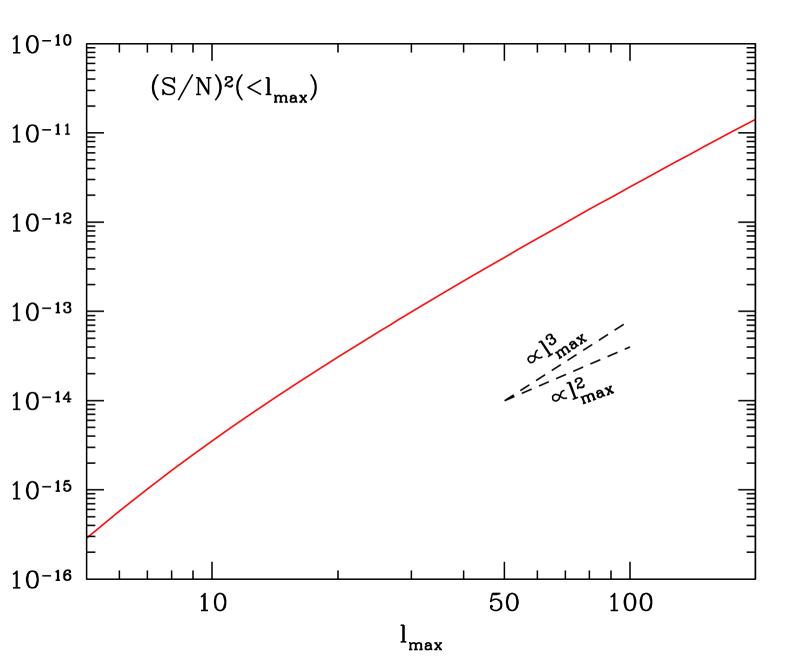
The signal-to-noise for the CMB trispectrum Tl3l4l1l2(L)superscriptsubscript𝑇subscript𝑙3subscript𝑙4subscript𝑙1subscript𝑙2𝐿T_{l_{3}l_{4}}^{l_{1}l_{2}}(L) summed up to a certain lmaxsubscript𝑙maxl_{\rm max} is 2002PhRvD..66f3008O

(SN)2(<lmax)l1>l2>l3>l4lmaxL|Tl3l4l1l2(L)|2(2L+1)Cl1Cl2Cl3Cl4annotatedsuperscript𝑆𝑁2absentsubscript𝑙maxsuperscriptsubscriptsubscript𝑙1subscript𝑙2subscript𝑙3subscript𝑙4subscript𝑙maxsubscript𝐿superscriptsuperscriptsubscript𝑇subscript𝑙3subscript𝑙4subscript𝑙1subscript𝑙2𝐿22𝐿1subscript𝐶subscript𝑙1subscript𝐶subscript𝑙2subscript𝐶subscript𝑙3subscript𝐶subscript𝑙4\left(\frac{S}{N}\right)^{2}\!\!(<l_{\rm max})\approx\sum_{l_{1}>l_{2}>l_{3}>l_{4}}^{l_{\rm max}}\sum_{L}\frac{|T_{l_{3}l_{4}}^{l_{1}l_{2}}(L)|^{2}}{(2L+1)C_{l_{1}}C_{l_{2}}C_{l_{3}}C_{l_{4}}} (44)

when cosmic variance dominates the errors. Otherwise, one shall include a contribution from the power spectrum of the detector noise to the Clsubscript𝐶𝑙C_{l}. Galactic foreground subtraction on a fraction 1fsky1subscript𝑓sky1-f_{\rm sky} would further reduce (S/N)2superscript𝑆𝑁2(S/N)^{2} by a factor of fskysubscript𝑓skyf_{\rm sky}.

Neglecting the ISW effect, the Sachs-Wolfe provides a useful order-of-magnitude estimate of the signal-to-noise as long as lmaxsubscript𝑙maxl_{\rm max} does not exceed 100less-than-or-similar-toabsent100\lesssim 100 1994ApJ…430..447G ; 2001PhRvD..63f3002K ; 2002PhRvD..66f3008O ; 2006PhRvD..73h3007K . The calculation is performed in Appendix B. We find that the signal-to-noise can be recast into the compact form

(SN)2(<lmax)annotatedsuperscript𝑆𝑁2absentsubscript𝑙max\displaystyle\left(\frac{S}{N}\right)^{2}\!\!(<l_{\rm max}) =92gNL2Aϕ2{161+1dxslmax3(x)tlmax(x)\displaystyle=\frac{9}{2}g_{\rm NL}^{2}A_{\phi}^{2}\left\{\frac{1}{6}\int_{-1}^{+1}\!\!dx\,s_{l_{\rm max}}^{3}(x)t_{l_{\rm max}}(x)\right.
+121+1dxrlmax2(x)slmax2(x)}\displaystyle\qquad+\left.\frac{1}{2}\int_{-1}^{+1}\!\!dx\,r_{l_{\rm max}}^{2}(x)s_{l_{\rm max}}^{2}(x)\right\} (45)

where the auxiliary functions rl(x)subscript𝑟𝑙𝑥r_{l}(x), sl(x)subscript𝑠𝑙𝑥s_{l}(x) and tl(x)subscript𝑡𝑙𝑥t_{l}(x) are defined as

rl(x)subscript𝑟𝑙𝑥\displaystyle r_{l}(x) =k=2l(2k+1)Pk(x)absentsuperscriptsubscript𝑘2𝑙2𝑘1subscript𝑃𝑘𝑥\displaystyle=\sum_{k=2}^{l}(2k+1)P_{k}(x) (46)
sl(x)subscript𝑠𝑙𝑥\displaystyle s_{l}(x) =k=2l(2k+1)k(k+1)Pk(x)absentsuperscriptsubscript𝑘2𝑙2𝑘1𝑘𝑘1subscript𝑃𝑘𝑥\displaystyle=\sum_{k=2}^{l}\frac{(2k+1)}{k(k+1)}P_{k}(x) (47)
tl(x)subscript𝑡𝑙𝑥\displaystyle t_{l}(x) =k=2l(2k+1)k(k+1)Pk(x).absentsuperscriptsubscript𝑘2𝑙2𝑘1𝑘𝑘1subscript𝑃𝑘𝑥\displaystyle=\sum_{k=2}^{l}(2k+1)k(k+1)P_{k}(x)\;. (48)

Here, Pl(x)subscript𝑃𝑙𝑥P_{l}(x) are Legendre polynomials. Note that we have excluded the monopole and dipole from the summation since these modes are unobservable. We have also assumed a nearly scale-invariant spectrum ns1subscript𝑛𝑠1n_{s}\approx 1.

Refer to caption
Figure 9: Signal-to-noise ratio squared for the CMB trispectrum as a function of the maximum multipole lmaxsubscript𝑙maxl_{\rm max}. We have assumed gNL=1subscript𝑔NL1g_{\rm NL}=1 and fsky=1subscript𝑓sky1f_{\rm sky}=1.

Figure. 9 shows the signal-to-noise ratio squared in the Sachs-Wolfe approximation for the CMB trispectrum assuming gNL=1subscript𝑔NL1g_{\rm NL}=1. Although this approximation breaks down for lmax100greater-than-or-equivalent-tosubscript𝑙max100l_{\rm max}\gtrsim 100, we have extended the calculation up to lmax=200subscript𝑙max200l_{\rm max}=200 so as to extrapolate more robustly the lmaxsubscript𝑙maxl_{\rm max}-dependence to small angular resolution. A power-law fit to (S/N)2superscript𝑆𝑁2(S/N)^{2} in the range 50lmax20050subscript𝑙max20050\leq l_{\rm max}\leq 200 gives

(SN)2(<lmax)2.43×10¹⁷gNL2(Aϕ109)2lmax2.6.similar-to-or-equalsannotatedsuperscript𝑆𝑁2absentsubscript𝑙max2.43superscript1017superscriptsubscript𝑔NL2superscriptsubscript𝐴italic-ϕsuperscript1092superscriptsubscript𝑙max2.6\left(\frac{S}{N}\right)^{2}\!\!(<l_{\rm max})\simeq 2.43\times 10^{-17}g_{\rm NL}^{2}\left(\frac{A_{\phi}}{10^{-9}}\right)^{2}l_{\rm max}^{2.6}\;. (49)

Our results appear consistent with the findings of 2002PhRvD..66f3008O shown in their Fig.2. However, our constant of proportionality is about 20-30 times larger, presumably because they adopted a lower fluctuation amplitude (compare also their prediction for the fNLsubscript𝑓NLf_{\rm NL} model with that of 2006PhRvD..73h3007K ). Adding the information encoded in temperature-polarization trispectra may enhance (S/N)2superscript𝑆𝑁2(S/N)^{2} by a factor of a few 2001PhRvD..64h3005H .

Assuming the scaling Eq.(49) persists well beyond the range over which the Sachs-Wolfe effect dominates, the minimum gNLsubscript𝑔NLg_{\rm NL} detectable at 1-σ𝜎\sigma level is gNL20similar-to-or-equalssubscript𝑔NL20g_{\rm NL}\simeq 20, 7.9, 3.2, 1.9 and 1.3×1041.3superscript1041.3\times 10^{4} for lmax=250subscript𝑙max250l_{\rm max}=250, 500, 1000, 1500 and 2000. A more realistic calculation should include the full radiation transfer function, detector noise etc. In this respect, detailed calculations have shown that, for the quadratic coupling fNLϕ2subscript𝑓NLsuperscriptitalic-ϕ2f_{\rm NL}\phi^{2}, (S/N)2superscript𝑆𝑁2(S/N)^{2} of the CMB bispectrum and trispectrum closely follows the behaviour obtained in the Sachs-Wolfe approximation 2002PhRvD..66f3008O ; 2006PhRvD..73h3007K . It seems reasonable, then, to expect that this is also true for gNLϕ3subscript𝑔NLsuperscriptitalic-ϕ3g_{\rm NL}\phi^{3}.

While our predictions are qualitative they show that, for the WMAP CMB temperature measurement  444http://map.gsfc.nasa.gov/ (which we approximate as a noise-free experiment with lmax250similar-tosubscript𝑙max250l_{\rm max}\sim 250), no detection of a significant trispectrum implies |gNL|2×10⁵subscript𝑔NL2superscript105|g_{\rm NL}|\leq 2\times 10^{5} at the 1-σ𝜎\sigma level. This is of the same order as the limit we derived from the QSO sample analyzed by 2008JCAP…08..031S . For a PLANCK-like experiment 555http://sci.esa.int/science-e/www/area/index.cfm?fareaid=17 (lmax1500similar-tosubscript𝑙max1500l_{\rm max}\sim 1500), no evidence for a trispectrum would imply |gNL|1.3×10⁴subscript𝑔NL1.3superscript104|g_{\rm NL}|\leq 1.3\times 10^{4} at the 1-σ𝜎\sigma level. This is comparable to the detection limit that could be achieved with an all-sky survey such as EUCLID.

V Effect of non-Gaussianity with non-zero fNLsubscript𝑓NLf_{\rm NL} and gNLsubscript𝑔NLg_{\rm NL}

In this Section, we examine the halo multiplicity function and large-scale bias in numerical simulations of structure formation with non-zero coupling parameters (fNL,gNL)=(±100,3×10⁵)subscript𝑓NLsubscript𝑔NLplus-or-minus1003superscript105(f_{\rm NL},g_{\rm NL})=(\pm 100,-3\times 10^{5}). We show that the results are consistent with those obtained from the simulations with non-vanishing gNLsubscript𝑔NLg_{\rm NL} solely.

V.1 Mass function

It is straightforward to calculate the fractional deviation from the Gaussian mass function, Eq.(18), to non-zero fNLsubscript𝑓NLf_{\rm NL} and gNLsubscript𝑔NLg_{\rm NL}. Again, we start with the MVJ formula and neglect second order corrections such as (σS3)2superscript𝜎subscript𝑆32(\sigma S_{3})^{2} etc. Adjusting the coefficient of the terms νσS3𝜈𝜎subscript𝑆3\nu\sigma S_{3} and ν2σ2S4superscript𝜈2superscript𝜎2subscript𝑆4\nu^{2}\sigma^{2}S_{4} to that of the small ν𝜈\nu expansion obtained by 2008JCAP…04..014L , we arrive at

R(ν,NL)𝑅𝜈NL\displaystyle R(\nu,{\rm NL}) =exp[ν33!σS3+ν44!σ2S4+ν2δσ8]absentsuperscript𝜈33𝜎subscript𝑆3superscript𝜈44superscript𝜎2subscript𝑆4superscript𝜈2𝛿subscript𝜎8\displaystyle=\exp\left[\frac{\nu^{3}}{3!}\sigma S_{3}+\frac{\nu^{4}}{4!}\sigma^{2}S_{4}+\nu^{2}\delta\sigma_{8}\right]
×{1ν2σS3ν6d(σS3)dlnν\displaystyle\quad\times\left\{1-\frac{\nu}{2}\sigma S_{3}-\frac{\nu}{6}\frac{d(\sigma S_{3})}{d\ln\nu}\right. (50)
ν24σ2S4ν24!d(σ2S4)dlnν},\displaystyle\qquad\quad\left.-\frac{\nu^{2}}{4}\sigma^{2}S_{4}-\frac{\nu^{2}}{4!}\frac{d(\sigma^{2}S_{4})}{d\ln\nu}\right\}\;,

where the shorthand notation NLNL{\rm NL} designates the combination (fNL,gNL)subscript𝑓NLsubscript𝑔NL(f_{\rm NL},g_{\rm NL}). In Fig. 10, this theoretical prediction is compared R(ν,NL)𝑅𝜈NLR(\nu,{\rm NL}) measured in non-Gaussian simulations of (fNL,gNL)=(±100,3×10⁵)subscript𝑓NLsubscript𝑔NLplus-or-minus1003superscript105(f_{\rm NL},g_{\rm NL})=(\pm 100,-3\times 10^{5}). We account for the fact that the amplitude of density fluctuations is renormalised by δσ80.0045𝛿subscript𝜎80.0045\delta\sigma_{8}\approx 0.0045. Fig. 10 demonstrates that our approximation is in good agreement with the data, although it slightly overestimates the effect at z=2𝑧2z=2 when fNL=100subscript𝑓NL100f_{\rm NL}=-100. For fNL=100subscript𝑓NL100f_{\rm NL}=100, the positive and negative contributions from the quadratic and cubic coupling, respectively, almost cancel each other and flatten the fractional deviation over most of the mass range probed by the simulations.

The scale-independent bias shift which arises from the change in the mean number density of haloes can again be estimated using the peak-background split. We find

ΔbI(NL)Δsubscript𝑏INL\displaystyle\Delta b_{\rm I}({\rm NL}) 1σ[13!(ν33ν)σ2S4+12(ν21)σS3.\displaystyle\approx-\frac{1}{\sigma}\biggl{[}\frac{1}{3!}\left(\nu^{3}-3\nu\right)\sigma^{2}S_{4}+\frac{1}{2}\left(\nu^{2}-1\right)\sigma S_{3}\biggr{.}
.+14!(ν38ν)d(σ2S4)dlnνν4!d2(σ2S4)dlnν2.\displaystyle\qquad\biggl{.}+\frac{1}{4!}\left(\nu^{3}-8\nu\right)\frac{d(\sigma^{2}S_{4})}{d\ln\nu}-\frac{\nu}{4!}\frac{d^{2}(\sigma^{2}S_{4})}{d\ln\nu^{2}}\biggr{.}
.+16(ν24)d(σS3)dlnν16d2(σS3)dlnν2.\displaystyle\qquad\biggl{.}+\frac{1}{6}\left(\nu^{2}-4\right)\frac{d(\sigma S_{3})}{d\ln\nu}-\frac{1}{6}\frac{d^{2}(\sigma S_{3})}{d\ln\nu^{2}}\biggr{.}
.+2νδσ8]\displaystyle\qquad\biggl{.}+2\nu\delta\sigma_{8}\biggr{]} (51)

at the first order in the nonlinear parameters fNLsubscript𝑓NLf_{\rm NL} and gNLsubscript𝑔NLg_{\rm NL}.

V.2 Bias

Having checked that the amount of non-Gaussianity in the mass function is also consistent with our simple theoretical expectation when both fNLsubscript𝑓NLf_{\rm NL} and gNLsubscript𝑔NLg_{\rm NL} are non-zero, we now turn to the clustering of dark matter haloes. As shown in Appendix A, the non-Gaussian correction to the halo power spectrum can be written down as

ΔPhh(k)Δsubscript𝑃hh𝑘\displaystyle\Delta P_{\rm hh}(k) =4fNLbL2δc(z)αM(k)Pϕ(k)absent4subscript𝑓NLsuperscriptsubscript𝑏L2subscript𝛿c𝑧subscript𝛼𝑀𝑘subscript𝑃italic-ϕ𝑘\displaystyle=4f_{\rm NL}b_{\rm L}^{2}\delta_{\rm c}(z)\alpha_{M}(k)P_{\phi}(k)
+4fNL2bL2δc2(z)Pϕ(k)+(gNL+43fNL2)4superscriptsubscript𝑓NL2superscriptsubscript𝑏L2superscriptsubscript𝛿c2𝑧subscript𝑃italic-ϕ𝑘subscript𝑔NL43superscriptsubscript𝑓NL2\displaystyle\quad+4f_{\rm NL}^{2}b_{\rm L}^{2}\delta_{\rm c}^{2}(z)P_{\phi}(k)+\left(g_{\rm NL}+\frac{4}{3}f_{\rm NL}^{2}\right)
×bL2δc2(z)S3(1)(M)αM(k)Pϕ(k).absentsuperscriptsubscript𝑏L2superscriptsubscript𝛿c2𝑧superscriptsubscript𝑆31𝑀subscript𝛼𝑀𝑘subscript𝑃italic-ϕ𝑘\displaystyle\qquad\times b_{\rm L}^{2}\delta_{\rm c}^{2}(z)S_{3}^{(1)}\!(M)\alpha_{M}(k)P_{\phi}(k)\;. (52)

If we set gNL=0subscript𝑔NL0g_{\rm NL}=0 and keep only the first two terms in the right-hand side, then the non-Gaussian (Eulerian) halo power spectrum can be cast into the form

Phh(k)=[b(M)+fNLbϕ(k)]2Pδ(k)subscript𝑃hh𝑘superscriptdelimited-[]𝑏𝑀subscript𝑓NLsubscript𝑏italic-ϕ𝑘2subscript𝑃𝛿𝑘P_{\rm hh}(k)=\bigl{[}b(M)+f_{\rm NL}b_{\phi}(k)\bigr{]}^{2}P_{\delta}(k) (53)

where the scale-dependent bias parameter bϕ(k)subscript𝑏italic-ϕ𝑘b_{\phi}(k) is

bϕ(k)=2[b(M)1]δc(z)αM1(k).subscript𝑏italic-ϕ𝑘2delimited-[]𝑏𝑀1subscript𝛿c𝑧superscriptsubscript𝛼𝑀1𝑘b_{\phi}(k)=2\bigl{[}b(M)-1\bigr{]}\delta_{\rm c}(z)\,\alpha_{M}^{-1}(k)\;. (54)

Note that reference 2008PhRvD..78l3519M obtained this relation by considering the halo power spectrum implied by a bias relation that is a local mapping of the density field. In practice, the term proportional to Pϕ(k)subscript𝑃italic-ϕ𝑘P_{\phi}(k) is negligible as it contributes only at very small wavenumber k0.001h1Mpcless-than-or-similar-to𝑘0.001superscript1Mpck\lesssim 0.001\ {\rm{\it h}^{-1}Mpc}. The third term in the right-hand side of Eq.(52) is derived in this paper for the first time. In the case gNL=0subscript𝑔NL0g_{\rm NL}=0, its magnitude relative to the term linear in fNLsubscript𝑓NLf_{\rm NL} is (1/3)fNLδc(z)S3(1)(M)13subscript𝑓NLsubscript𝛿c𝑧superscriptsubscript𝑆31𝑀(1/3)f_{\rm NL}\delta_{\rm c}(z)S_{3}^{(1)}\!(M), which is approximately 0.03similar-toabsent0.03\sim 0.03 at redshift z=1.8𝑧1.8z=1.8 and for a mass scale M=1013M/h𝑀superscript1013subscriptMdirect-productM=10^{13}\ {\rm M_{\odot}/{\it h}}. Although its contribution becomes increasingly important at higher redshift, it is fairly small for the values of fNLsubscript𝑓NLf_{\rm NL} considered here. Consequently, we shall employ the approximation

Δb(k,NL)Δ𝑏𝑘NL\displaystyle\Delta b(k,{\rm NL}) =ϵκΔbκ(k,gNL)+Δbκ(k,fNL)absentsubscriptitalic-ϵ𝜅Δsubscript𝑏𝜅𝑘subscript𝑔NLΔsubscript𝑏𝜅𝑘subscript𝑓NL\displaystyle=\epsilon_{\kappa}\,\Delta b_{\kappa}(k,g_{\rm NL})+\Delta b_{\kappa}(k,f_{\rm NL})
+[ΔbI(NL)+ϵI].delimited-[]Δsubscript𝑏INLsubscriptitalic-ϵI\displaystyle\quad+\bigl{[}\Delta b_{\rm I}({\rm NL})+\epsilon_{\rm I}\bigr{]}\;. (55)

to describe the non-Gaussian bias of dark matter haloes.
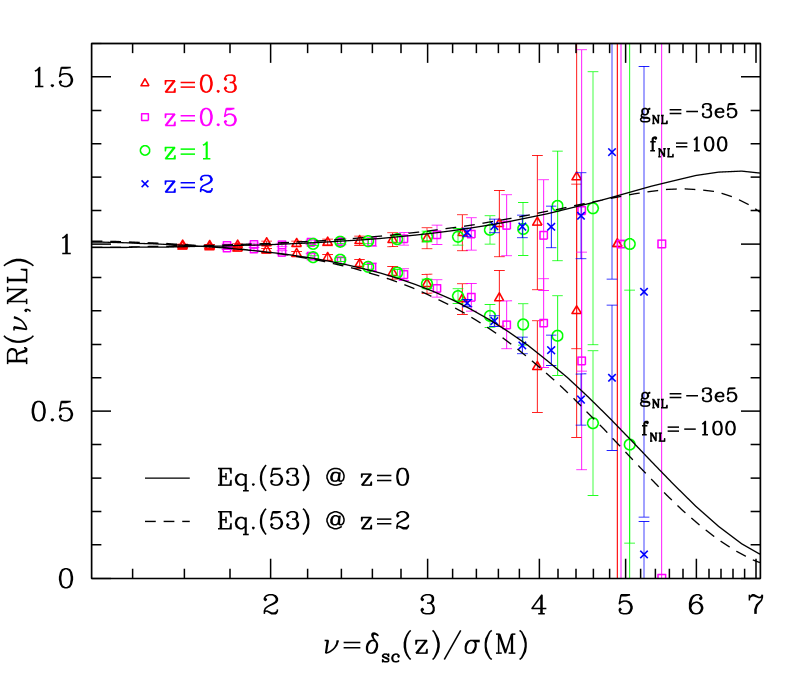
Refer to caption
Figure 10: Fractional correction to the Gaussian multiplicity function of dark matter haloes as a function of the peak height ν(M,z)𝜈𝑀𝑧\nu(M,z) for fNL=±100subscript𝑓NLplus-or-minus100f_{\rm NL}=\pm 100 and a cubic coupling parameter gNL=3×10⁵subscript𝑔NL3superscript105g_{\rm NL}=-3\times 10^{5}. The solid and dashed curves show the theoretical prediction Eq.(V.1) at z=0𝑧0z=0 and 2, respectively. Error bars denote Poisson errors.
Refer to caption
Figure 11: Non-Gaussian bias correction measured in the simulations with (fNL,gNL)=(±100,3×10⁵)subscript𝑓NLsubscript𝑔NLplus-or-minus1003superscript105(f_{\rm NL},g_{\rm NL})=(\pm 100,-3\times 10^{5}) for haloes of mass M>2×10¹³M/h𝑀2superscript1013subscriptMdirect-productM>2\times 10^{13}\ {\rm M_{\odot}/{\it h}}. Error bars are not shown as the data points are averaged over two realisations solely.

The quadratic coupling fNLϕ2subscript𝑓NLsuperscriptitalic-ϕ2f_{\rm NL}\phi^{2} also affect the matter power spectrum at leading order 2004PhRvD..69j3513S ; 2008MNRAS.390..438G , positive values of fNLsubscript𝑓NLf_{\rm NL} increasing the small scale power. However, the relative size of this k𝑘k-dependent correction, βm(k,fNL)subscript𝛽m𝑘subscript𝑓NL\beta_{\rm m}(k,f_{\rm NL}), is at a per cent level only in the weakly nonlinear regime k0.1hMpc1less-than-or-similar-to𝑘0.1superscriptMpc1k\lesssim 0.1\ {\rm{\it h}Mpc^{-1}} 2008PhRvD..78l3534T ; 2009MNRAS.396…85D and fades rapidly as one goes to larger scales. We will thus neglect it in what follows.

In Fig. 11, the result of measuring ratios of auto- and cross-power spectra in the simulations with (fNL,gNL)=(±100,3×10⁵)subscript𝑓NLsubscript𝑔NLplus-or-minus1003superscript105(f_{\rm NL},g_{\rm NL})=(\pm 100,-3\times 10^{5}) is shown at 0<z<1.50𝑧1.50<z<1.5 for the haloes with M>2×10¹³M/h𝑀2superscript1013subscriptMdirect-productM>2\times 10^{13}\ {\rm M_{\odot}/{\it h}}. We do not quote error bars since the data points are obtained by averaging over two realisations only. The solid and dashed curves show the theoretical prediction Eq. (55). The value of the multiplicative factor ϵκ(b,gNL)subscriptitalic-ϵ𝜅𝑏subscript𝑔NL\epsilon_{\kappa}(b,g_{\rm NL}) was obtained from the four-parameter formula Eq.(31), while ΔbI+ϵIΔsubscript𝑏Isubscriptitalic-ϵI\Delta b_{\rm I}+\epsilon_{\rm I} was individually fitted for each halo sample over the wavenumber range 0.005<k<0.03hMpc10.005𝑘0.03superscriptMpc10.005<k<0.03\ {\rm{\it h}Mpc^{-1}}. As can be seen, the theoretical expectation Eq. (55) agrees reasonably well with the numerical data. This demonstrates that the range of validity of the non-Gaussian bias formula Eq. (30) extends to smaller values of gNLsubscript𝑔NLg_{\rm NL} as well as models with non-vanishing fNLsubscript𝑓NLf_{\rm NL} and gNLsubscript𝑔NLg_{\rm NL}.

The lowest order, k𝑘k-dependent corrections to the Gaussian bias induced by the quadratic and the cubic coupling are fully degenerated in the halo power spectrum as they both scale as αM1(k)k2T(k)1proportional-tosuperscriptsubscript𝛼𝑀1𝑘superscript𝑘2𝑇superscript𝑘1\alpha_{M}^{-1}(k)\propto k^{-2}T(k)^{-1}. For the values of fNLsubscript𝑓NLf_{\rm NL} and gNLsubscript𝑔NLg_{\rm NL} and the halo mass range considered here, the ratio Δbκ(k,gNL)/Δbκ(k,fNL)Δsubscript𝑏𝜅𝑘subscript𝑔NLΔsubscript𝑏𝜅𝑘subscript𝑓NL\Delta b_{\kappa}(k,g_{\rm NL})/\Delta b_{\kappa}(k,f_{\rm NL}) increases approximately from 0.25 to 0.5 when the redshift increases from z=0𝑧0z=0 to 2. It is unclear whether higher order corrections could help breaking such a degeneracy. A more promising alternative may be to measure the bispectrum of dark matter haloes, which carries much more information about the shape of the primordial three-point function than the power spectrum of bias tracers 2009arXiv0904.0497J ; 2009arXiv0905.0717S . However, this is beyond the scope of this paper.

VI Discussion

In this paper we explored the effect of a local cubic coupling gNLϕ3subscript𝑔NLsuperscriptitalic-ϕ3g_{\rm NL}\phi^{3} on the mass function and bias of dark matter haloes. We derived analytical expressions for these statistics and tested them against the outcome of numerical simulations.

We showed that current theoretical predictions of the non-Gaussian correction to the mass function reasonably agree with the simulations. The LV formula 2008JCAP…04..014L appears to provide a better fit to the data than the MVJ formula 2000ApJ…541…10M , in agreement with some of the literature on the subject 2007MNRAS.376..343K ; 2008PhRvD..77l3514D . The two approximations can be combined to provide an accurate description if one adjusts the low-ν𝜈\nu expansion of the latter so as to match that of the former.

We found that the magnitude of the non-Gaussian scale-dependent bias Δbκ(k,gNL)Δsubscript𝑏𝜅𝑘subscript𝑔NL\Delta b_{\kappa}(k,g_{\rm NL}) is suppressed relative to a theoretical prediction based on the statistics of highly overdense regions, even on linear scales k0.01hMpc1less-than-or-similar-to𝑘0.01superscriptMpc1k\lesssim 0.01\ {\rm{\it h}Mpc^{-1}}. This suppression is stronger for the low biased samples b3less-than-or-similar-to𝑏3b\lesssim 3 and, at fixed value of b𝑏b, for positive values of gNLsubscript𝑔NLg_{\rm NL}. We were able to fit the measured halo bias at the expense of introducing two free parameters, ϵκsubscriptitalic-ϵ𝜅\epsilon_{\kappa} and ϵIsubscriptitalic-ϵI\epsilon_{\rm I}, that depend mostly on the halo bias b(M)𝑏𝑀b(M) and the coupling parameter gNLsubscript𝑔NLg_{\rm NL}. These parameters quantify the departure from the theoretical scale-dependent and scale-independent non-Gaussian bias correction, respectively. We provide a simple fitting formula for ϵκ(b,gNL)subscriptitalic-ϵ𝜅𝑏subscript𝑔NL\epsilon_{\kappa}(b,g_{\rm NL}), Eq.(31), which should be used when analyzing observational data. In non-Gaussian simulations of the fNLsubscript𝑓NLf_{\rm NL} type, the data also hint at a (possibly fNLsubscript𝑓NLf_{\rm NL}-dependent) suppression of the non-Gaussian scale-dependent bias relative to theory for wavemodes k0.03hMpc1less-than-or-similar-to𝑘0.03superscriptMpc1k\lesssim 0.03\ {\rm{\it h}Mpc^{-1}} 2009MNRAS.396…85D ; 2008arXiv0811.4176P ; 2009arXiv0902.2013G , but the effect is much weaker than seen in our simulations of gNLsubscript𝑔NLg_{\rm NL} models. Clearly, these results require a better theoretical modelling of the non-Gaussian halo bias.

Reference 2009arXiv0902.2013G argued that both the MVJ and LV analytic formula can be reconciled with measurements of the non-Gaussian fractional correction to the mass function once non-spherical collapse is included. In practice, the critical density for collapse is replaced by δcqδcsubscript𝛿c𝑞subscript𝛿c\delta_{\rm c}\rightarrow\sqrt{q}\delta_{\rm c}, where the value q=0.75𝑞0.75q=0.75 is obtained from a fit to the mass function measured in simulations 2002MNRAS.329…61S . Reference 2009arXiv0903.1251M claimed that such a relation is a consequence of the diffusive nature of the critical threshold for collapse. Their model predicts q0.8similar-to-or-equals𝑞0.8q\simeq 0.8, in good agreement with the findings of 2009arXiv0902.2013G . However, we found that substituting δcqδcsubscript𝛿c𝑞subscript𝛿c\delta_{\rm c}\rightarrow\sqrt{q}\delta_{\rm c} in Eq.(18) only modestly improve the agreement with the data. Regarding the non-Gaussian bias, it is not obvious how one could justify the replacement δcqδcsubscript𝛿c𝑞subscript𝛿c\delta_{\rm c}\rightarrow\sqrt{q}\delta_{\rm c} given that the linear bias of our (Gaussian) halo samples converges towards the spherical collapse prediction ν2/δcsuperscript𝜈2subscript𝛿c\nu^{2}/\delta_{\rm c} for large peak height.

A important ingredient is the choice of the halo identification algorithm. While we used a spherical overdensity (SO) finder, reference 2009arXiv0903.1251M considered a Friends-of-Friends (FoF) finder with a linking length b=0.2𝑏0.2b=0.2. The question of how the spherical overdensity masses can be mapped onto friends-of-friends masses remains a matter of debate 2009ApJ…692..217L . Clealy however, since the peak height depends on the halo mass M𝑀M through the variance σ(M)𝜎𝑀\sigma(M), any systematic difference will be reflected in the value of ν𝜈\nu associated to a specific halo sample. This will in turn affects the size of the fractional deviation from the Gaussian mass function at some specified peak height. The sensitivity of the non-Gaussian mass function and bias to the halo finder will be presented elsewhere.

The observational bound on fNLsubscript𝑓NLf_{\rm NL} inferred by 2008JCAP…08..031S from the clustering of a high redshift sample of quasars can be straightforwardly translated into a limit on gNLsubscript𝑔NLg_{\rm NL} since Δbκ(k,gNL)Δsubscript𝑏𝜅𝑘subscript𝑔NL\Delta b_{\kappa}(k,g_{\rm NL}) also scales as k2T(k)1superscript𝑘2𝑇superscript𝑘1k^{-2}T(k)^{-1} at low wavenumber. We have obtained

3.5×10⁵<gNL<+8.2×10⁵(95%).3.5superscript105subscript𝑔NL8.2superscript105percent95-3.5\times 10^{5}<g_{\rm NL}<+8.2\times 10^{5}~{}~{}(95\%). (56)

These are the first limits derived on gNLsubscript𝑔NLg_{\rm NL}. While they are too weak to provide interesting constraints on inflationary scenarios such as the curvaton model, future all-sky redshift surveys should improve them by a factor of 100similar-toabsent100\sim 100. Future CMB observations, including PLANCK, should also improve the limits derived here by an order of magnitude. With these improvements we expect that, in the next decade, realistic models of cubic type non-Gaussianity will be tested with real observations.

Acknowledgements

We thank Paolo Creminelli and Leonardo Senatore for useful discussions. We acknowledge support from the Swiss National Foundation under contract No. 200021-116696/1 and WCU grant R32-2008-000-10130-0.

Appendix A Non-Gaussian bias in the high peak limit

In this Appendix, we detail the derivation of the scale-dependent bias correction induced by the gNLsubscript𝑔NLg_{\rm NL} coupling to the two-point correlation of dark matter haloes. We follow 2008ApJ…677L..77M and approximate the latter by the two-point correlation ξhh(𝐫)subscript𝜉hh𝐫\xi_{\rm hh}({\bf r}) of regions of the smoothed density field δMsubscript𝛿𝑀\delta_{M} with a peak height ν1much-greater-than𝜈1\nu\gg 1.

A.1 case gNL0subscript𝑔NL0g_{\rm NL}\neq 0 only

In this case, only the four-point correlations of the density field contribute at the first order. The leading-order correction to the correlation of tresholded regions thus reads as

Δξhh=ν4σ4[13ξ(4)(𝐱1,𝐱1,𝐱1,𝐱2)+14ξ(4)(𝐱1,𝐱1,𝐱2,𝐱2)].Δsubscript𝜉hhsuperscript𝜈4superscript𝜎4delimited-[]13superscript𝜉4subscript𝐱1subscript𝐱1subscript𝐱1subscript𝐱214superscript𝜉4subscript𝐱1subscript𝐱1subscript𝐱2subscript𝐱2\Delta\xi_{\rm hh}=\frac{\nu^{4}}{\sigma^{4}}\left[\frac{1}{3}\xi^{(4)}({\bf x}_{1},{\bf x}_{1},{\bf x}_{1},{\bf x}_{2})+\frac{1}{4}\xi^{(4)}({\bf x}_{1},{\bf x}_{1},{\bf x}_{2},{\bf x}_{2})\right]\;. (57)

The four-point correlations ξ(4)superscript𝜉4\xi^{(4)} are Fourier transform of the trispectrum of the density field, Tδ(𝐤1,𝐤2,𝐤3,𝐤4)subscript𝑇𝛿subscript𝐤1subscript𝐤2subscript𝐤3subscript𝐤4T_{\delta}({\bf k}_{1},{\bf k}_{2},{\bf k}_{3},{\bf k}_{4}), with conservation of momentum enforced. Linearly extrapolating the density field to present epoch, the latter can be expressed as

Tδ(𝐤1,𝐤2,𝐤3,𝐤4)=(i=14αM(ki))TΦ(𝐤1,𝐤2,𝐤3,𝐤4),subscript𝑇𝛿subscript𝐤1subscript𝐤2subscript𝐤3subscript𝐤4superscriptsubscriptproduct𝑖14subscript𝛼𝑀subscript𝑘𝑖subscript𝑇Φsubscript𝐤1subscript𝐤2subscript𝐤3subscript𝐤4T_{\delta}({\bf k}_{1},{\bf k}_{2},{\bf k}_{3},{\bf k}_{4})=\left(\prod_{i=1}^{4}\alpha_{M}(k_{i})\right)\,T_{\Phi}({\bf k}_{1},{\bf k}_{2},{\bf k}_{3},{\bf k}_{4})\;, (58)

where the expression for the trispectrum of primordial curvature perturbation

TΦ(𝐤1,𝐤2,𝐤3,𝐤4)=6gNL[Pϕ(k1)Pϕ(k2)Pϕ(k3)+(cyclic)]subscript𝑇Φsubscript𝐤1subscript𝐤2subscript𝐤3subscript𝐤46subscript𝑔NLdelimited-[]subscript𝑃italic-ϕsubscript𝑘1subscript𝑃italic-ϕsubscript𝑘2subscript𝑃italic-ϕsubscript𝑘3(cyclic)T_{\Phi}({\bf k}_{1},{\bf k}_{2},{\bf k}_{3},{\bf k}_{4})=6g_{\rm NL}\bigl{[}P_{\phi}(k_{1})P_{\phi}(k_{2})P_{\phi}(k_{3})+\mbox{(cyclic)}\bigr{]} (59)

follows straightforwardly from the Fourier mode relation

Φ(𝐤)=ϕ(𝐤)+gNLd3k1(2π)3d3k2(2π)3ϕ(𝐤1)ϕ(𝐤2)ϕ(𝐤𝐤1𝐤2).Φ𝐤italic-ϕ𝐤subscript𝑔NLsuperscript𝑑3subscript𝑘1superscript2𝜋3superscript𝑑3subscript𝑘2superscript2𝜋3italic-ϕsubscript𝐤1italic-ϕsubscript𝐤2italic-ϕ𝐤subscript𝐤1subscript𝐤2\Phi({\bf k})=\phi({\bf k})+g_{\rm NL}\!\int\!\!\frac{d^{3}k_{1}}{(2\pi)^{3}}\!\int\!\!\frac{d^{3}k_{2}}{(2\pi)^{3}}\phi({\bf k}_{1})\phi({\bf k}_{2})\phi({\bf k}-{\bf k}_{1}-{\bf k}_{2})\;. (60)

Density and curvature perturbations are related through the Poisson equation, whose scale-dependence is reflected in the function αM(k)=αR(k,z=0)subscript𝛼𝑀𝑘subscript𝛼𝑅𝑘𝑧0\alpha_{M}(k)=\alpha_{R}(k,z=0) defined in Eq. (6). Combining these relations gives

ξ(4)(𝐱1,𝐱1,𝐱1,𝐱2)superscript𝜉4subscript𝐱1subscript𝐱1subscript𝐱1subscript𝐱2\displaystyle\xi^{(4)}({\bf x}_{1},{\bf x}_{1},{\bf x}_{1},{\bf x}_{2}) =6gNL(i=13d3ki(2π)3αM(ki)Pϕ(ki))[1+3Pϕ(k123)Pϕ(k3)]αM(k123)ei𝐤123𝐫absent6subscript𝑔NLsuperscriptsubscriptproduct𝑖13superscript𝑑3subscript𝑘𝑖superscript2𝜋3subscript𝛼𝑀subscript𝑘𝑖subscript𝑃italic-ϕsubscript𝑘𝑖delimited-[]13subscript𝑃italic-ϕsubscript𝑘123subscript𝑃italic-ϕsubscript𝑘3subscript𝛼𝑀subscript𝑘123superscript𝑒𝑖subscript𝐤123𝐫\displaystyle=6g_{\rm NL}\left(\prod_{i=1}^{3}\int\!\!\frac{d^{3}k_{i}}{(2\pi)^{3}}\,\alpha_{M}(k_{i})P_{\phi}(k_{i})\right)\left[1+3\,\frac{P_{\phi}(k_{123})}{P_{\phi}(k_{3})}\right]\alpha_{M}(k_{123})\,e^{i{\bf k}_{123}\cdot{\bf r}} (61)
ξ(4)(𝐱1,𝐱1,𝐱2,𝐱2)superscript𝜉4subscript𝐱1subscript𝐱1subscript𝐱2subscript𝐱2\displaystyle\xi^{(4)}({\bf x}_{1},{\bf x}_{1},{\bf x}_{2},{\bf x}_{2}) =6gNL(i=13d3ki(2π)3αM(ki)Pϕ(ki))[1+2Pϕ(k123)Pϕ(k1)+Pϕ(k123)Pϕ(k3)]αM(k123)ei𝐤12𝐫,absent6subscript𝑔NLsuperscriptsubscriptproduct𝑖13superscript𝑑3subscript𝑘𝑖superscript2𝜋3subscript𝛼𝑀subscript𝑘𝑖subscript𝑃italic-ϕsubscript𝑘𝑖delimited-[]12subscript𝑃italic-ϕsubscript𝑘123subscript𝑃italic-ϕsubscript𝑘1subscript𝑃italic-ϕsubscript𝑘123subscript𝑃italic-ϕsubscript𝑘3subscript𝛼𝑀subscript𝑘123superscript𝑒𝑖subscript𝐤12𝐫\displaystyle=6g_{\rm NL}\left(\prod_{i=1}^{3}\int\!\!\frac{d^{3}k_{i}}{(2\pi)^{3}}\,\alpha_{M}(k_{i})P_{\phi}(k_{i})\right)\left[1+2\frac{P_{\phi}(k_{123})}{P_{\phi}(k_{1})}+\frac{P_{\phi}(k_{123})}{P_{\phi}(k_{3})}\right]\alpha_{M}(k_{123})\,e^{i{\bf k}_{12}\cdot{\bf r}}\;, (62)

where we have defined 𝐤ijl=𝐤i+𝐤j++𝐤lsubscript𝐤𝑖𝑗𝑙subscript𝐤𝑖subscript𝐤𝑗subscript𝐤𝑙{\bf k}_{ij\cdots l}={\bf k}_{i}+{\bf k}_{j}+\,\cdots\,+{\bf k}_{l} for shorthand convenience. Since we will examine the effect of non-Gaussianity on Fourier space statistics only, we take the Fourier transform of the four-point functions. After some simplification, we arrive at

d3rξ(4)(𝐱1,𝐱1,𝐱1,𝐱2)ei𝐤𝐫superscript𝑑3𝑟superscript𝜉4subscript𝐱1subscript𝐱1subscript𝐱1subscript𝐱2superscript𝑒𝑖𝐤𝐫\displaystyle\int\!\!d^{3}r\,\xi^{(4)}({\bf x}_{1},{\bf x}_{1},{\bf x}_{1},{\bf x}_{2})e^{-i{\bf k}\cdot{\bf r}} =6gNLαM(k)Pϕ(k)d3k1(2π)3αM(k1)Pϕ(k1)d3k2(2π)3αM(k2)Pϕ(k2)absent6subscript𝑔NLsubscript𝛼𝑀𝑘subscript𝑃italic-ϕ𝑘superscript𝑑3subscript𝑘1superscript2𝜋3subscript𝛼𝑀subscript𝑘1subscript𝑃italic-ϕsubscript𝑘1superscript𝑑3subscript𝑘2superscript2𝜋3subscript𝛼𝑀subscript𝑘2subscript𝑃italic-ϕsubscript𝑘2\displaystyle=6g_{\rm NL}\alpha_{M}(k)P_{\phi}(k)\int\!\!\frac{d^{3}k_{1}}{(2\pi)^{3}}\alpha_{M}(k_{1})P_{\phi}(k_{1})\int\!\!\frac{d^{3}k_{2}}{(2\pi)^{3}}\alpha_{M}(k_{2})P_{\phi}(k_{2})
×αM(|𝐤+𝐤12|)[3+Pϕ(|𝐤+𝐤12|)Pϕ(k)]absentsubscript𝛼𝑀𝐤subscript𝐤12delimited-[]3subscript𝑃italic-ϕ𝐤subscript𝐤12subscript𝑃italic-ϕ𝑘\displaystyle\qquad\times\alpha_{M}\bigl{(}|{\bf k}+{\bf k}_{12}|\bigr{)}\left[3+\frac{P_{\phi}\bigl{(}|{\bf k}+{\bf k}_{12}|\bigr{)}}{P_{\phi}(k)}\right] (63)
d3rξ(4)(𝐱1,𝐱1,𝐱2,𝐱2)ei𝐤𝐫superscript𝑑3𝑟superscript𝜉4subscript𝐱1subscript𝐱1subscript𝐱2subscript𝐱2superscript𝑒𝑖𝐤𝐫\displaystyle\int\!\!d^{3}r\,\xi^{(4)}({\bf x}_{1},{\bf x}_{1},{\bf x}_{2},{\bf x}_{2})e^{-i{\bf k}\cdot{\bf r}} =6gNLd3k1(2π)3αM(k1)αM(|𝐤+𝐤1|)Pϕ(k1)Pϕ(|𝐤+𝐤1|)d3k2(2π)3αM(k2)absent6subscript𝑔NLsuperscript𝑑3subscript𝑘1superscript2𝜋3subscript𝛼𝑀subscript𝑘1subscript𝛼𝑀𝐤subscript𝐤1subscript𝑃italic-ϕsubscript𝑘1subscript𝑃italic-ϕ𝐤subscript𝐤1superscript𝑑3subscript𝑘2superscript2𝜋3subscript𝛼𝑀subscript𝑘2\displaystyle=6g_{\rm NL}\int\!\!\frac{d^{3}k_{1}}{(2\pi)^{3}}\alpha_{M}(k_{1})\alpha_{M}(|{\bf k}+{\bf k}_{1}|)P_{\phi}(k_{1})P_{\phi}\bigl{(}|{\bf k}+{\bf k}_{1}|\bigr{)}\int\!\!\frac{d^{3}k_{2}}{(2\pi)^{3}}\alpha_{M}(k_{2})
×αM(|𝐤+𝐤2|)Pϕ(k2)[1+2Pϕ(|𝐤+𝐤2|)Pϕ(|𝐤+𝐤1|)+Pϕ(|𝐤+𝐤2|)Pϕ(k2)].absentsubscript𝛼𝑀𝐤subscript𝐤2subscript𝑃italic-ϕsubscript𝑘2delimited-[]12subscript𝑃italic-ϕ𝐤subscript𝐤2subscript𝑃italic-ϕ𝐤subscript𝐤1subscript𝑃italic-ϕ𝐤subscript𝐤2subscript𝑃italic-ϕsubscript𝑘2\displaystyle\qquad\times\alpha_{M}\bigl{(}|{\bf k}+{\bf k}_{2}|\bigr{)}P_{\phi}(k_{2})\left[1+2\frac{P_{\phi}\bigl{(}|{\bf k}+{\bf k}_{2}|\bigr{)}}{P_{\phi}\bigl{(}|{\bf k}+{\bf k}_{1}|\bigr{)}}+\frac{P_{\phi}\bigl{(}|{\bf k}+{\bf k}_{2}|\bigr{)}}{P_{\phi}(k_{2})}\right]\;. (64)

For realistic values of the spectral index (ns1similar-tosubscript𝑛𝑠1n_{s}\sim 1), the products αM(|𝐤+𝐤i|)Pϕ(|𝐤+𝐤i|)subscript𝛼𝑀𝐤subscript𝐤𝑖subscript𝑃italic-ϕ𝐤subscript𝐤𝑖\alpha_{M}(|{\bf k}+{\bf k}_{i}|)P_{\phi}(|{\bf k}+{\bf k}_{i}|) appearing in the right-hand side of the above equalities formally diverges whenever 𝐤+𝐤1=0𝐤subscript𝐤10{\bf k}+{\bf k}_{1}=0 due to the ultraviolet divergence of Pϕ(k)subscript𝑃italic-ϕ𝑘P_{\phi}(k). To cure this problem, one can set Pϕ(k)=0subscript𝑃italic-ϕ𝑘0P_{\phi}(k)=0 for sufficiently small wavenumbers or excise a thin shell centred at wavenumber kisubscript𝑘𝑖k_{i} from the integral. In the large-scale limit kkimuch-less-than𝑘subscript𝑘𝑖k\ll k_{i}, the ratio Pϕ(|𝐤+𝐤i|)/Pϕ(k)subscript𝑃italic-ϕ𝐤subscript𝐤𝑖subscript𝑃italic-ϕ𝑘P_{\phi}(|{\bf k}+{\bf k}_{i}|)/P_{\phi}(k) vanishes whereas Pϕ(|𝐤+𝐤i|)/Pϕ(ki)subscript𝑃italic-ϕ𝐤subscript𝐤𝑖subscript𝑃italic-ϕsubscript𝑘𝑖P_{\phi}(|{\bf k}+{\bf k}_{i}|)/P_{\phi}(k_{i}) tends towards unity. In this case, the above expressions reduce to

d3rξ(4)(𝐱1,𝐱1,𝐱1,𝐱2)ei𝐤𝐫3gNLσ4S3(1)(M)αM(k)Pϕ(k)+6gNLαM(k)d3k1(2π)3αM(k1)Pϕ(k1)d3k2(2π)3αM(k2)Pϕ(k2)αM(k12)Pϕ(k12),superscript𝑑3𝑟superscript𝜉4subscript𝐱1subscript𝐱1subscript𝐱1subscript𝐱2superscript𝑒𝑖𝐤𝐫3subscript𝑔NLsuperscript𝜎4superscriptsubscript𝑆31𝑀subscript𝛼𝑀𝑘subscript𝑃italic-ϕ𝑘6subscript𝑔NLsubscript𝛼𝑀𝑘superscript𝑑3subscript𝑘1superscript2𝜋3subscript𝛼𝑀subscript𝑘1subscript𝑃italic-ϕsubscript𝑘1superscript𝑑3subscript𝑘2superscript2𝜋3subscript𝛼𝑀subscript𝑘2subscript𝑃italic-ϕsubscript𝑘2subscript𝛼𝑀subscript𝑘12subscript𝑃italic-ϕsubscript𝑘12\int\!\!d^{3}r\,\xi^{(4)}({\bf x}_{1},{\bf x}_{1},{\bf x}_{1},{\bf x}_{2})e^{-i{\bf k}\cdot{\bf r}}\approx 3g_{\rm NL}\,\sigma^{4}S_{3}^{(1)}\!(M)\,\alpha_{M}(k)P_{\phi}(k)\\ +6g_{\rm NL}\alpha_{M}(k)\int\!\!\frac{d^{3}k_{1}}{(2\pi)^{3}}\alpha_{M}(k_{1})P_{\phi}(k_{1})\int\!\!\frac{d^{3}k_{2}}{(2\pi)^{3}}\alpha_{M}(k_{2})P_{\phi}(k_{2})\alpha_{M}(k_{12})P_{\phi}(k_{12})\;, (65)

and

d3rξ(4)(𝐱1,𝐱1,𝐱2,𝐱2)ei𝐤𝐫24gNLσ2d3k1(2π)3αM2(k1)Pϕ2(k1).superscript𝑑3𝑟superscript𝜉4subscript𝐱1subscript𝐱1subscript𝐱2subscript𝐱2superscript𝑒𝑖𝐤𝐫24subscript𝑔NLsuperscript𝜎2superscript𝑑3subscript𝑘1superscript2𝜋3superscriptsubscript𝛼𝑀2subscript𝑘1superscriptsubscript𝑃italic-ϕ2subscript𝑘1\hbox to0.0pt{$\displaystyle\int\!\!d^{3}r\,\xi^{(4)}({\bf x}_{1},{\bf x}_{1},{\bf x}_{2},{\bf x}_{2})e^{-i{\bf k}\cdot{\bf r}}$\hss}\\ \approx 24g_{\rm NL}\,\sigma^{2}\int\!\!\frac{d^{3}k_{1}}{(2\pi)^{3}}\,\alpha_{M}^{2}(k_{1})P_{\phi}^{2}(k_{1})\;. (66)

Only the first term in the right-hand side of Eq.(65) is not well behaved in the limit k0𝑘0k\rightarrow 0 where it becomes proportional to kns2superscript𝑘subscript𝑛𝑠2k^{n_{s}-2}. The second scales as k2superscript𝑘2k^{2}, while the Fourier transform of ξ(4)(𝐱1,𝐱1,𝐱2,𝐱2)superscript𝜉4subscript𝐱1subscript𝐱1subscript𝐱2subscript𝐱2\xi^{(4)}({\bf x}_{1},{\bf x}_{1},{\bf x}_{2},{\bf x}_{2}) asymptotes to a constant. A similar decomposition also arises in fNLsubscript𝑓NLf_{\rm NL} models. For this type of non-Gaussianity, the first order correction is furnished by the three-point function ξ(3)(𝐱1,𝐱1,𝐱2)superscript𝜉3subscript𝐱1subscript𝐱1subscript𝐱2\xi^{(3)}({\bf x}_{1},{\bf x}_{1},{\bf x}_{2}), whose Fourier transform can be split into the familiar term 2fNLσ2αM(k)Pϕ(k)2subscript𝑓NLsuperscript𝜎2subscript𝛼𝑀𝑘subscript𝑃italic-ϕ𝑘2f_{\rm NL}\sigma^{2}\alpha_{M}(k)P_{\phi}(k), and a second piece given by

12fNLαM(k)d3k1(2π)3αM2(k1)Pϕ2(k1).12subscript𝑓NLsubscript𝛼𝑀𝑘superscript𝑑3subscript𝑘1superscript2𝜋3superscriptsubscript𝛼𝑀2subscript𝑘1superscriptsubscript𝑃italic-ϕ2subscript𝑘1\frac{1}{2}f_{\rm NL}\alpha_{M}(k)\int\!\!\frac{d^{3}k_{1}}{(2\pi)^{3}}\,\alpha_{M}^{2}(k_{1})P_{\phi}^{2}(k_{1})\;. (67)

In both quadratic and cubic local non-Gaussianity, the term proportional to αM(k)subscript𝛼𝑀𝑘\alpha_{M}(k) can be neglected since, at the pivot point k=k0𝑘subscript𝑘0k=k_{0}, its magnitude relative to the term involving αM(k)Pϕ(k)subscript𝛼𝑀𝑘subscript𝑃italic-ϕ𝑘\alpha_{M}(k)P_{\phi}(k) is only 𝒪(0.01)𝒪0.01{\cal O}(0.01) and 𝒪(106)𝒪superscript106{\cal O}(10^{-6}), respectively. Moreover, it decreases as one goes to larger scales. By contrast, it is not so obvious how to handle the term (66). In the non-Gaussian halo power spectrum, this term would appear multiplied by ν4/(4σ4)superscript𝜈44superscript𝜎4\nu^{4}/(4\sigma^{4}),

6gNLbL2δc2(z)σ2d3k1(2π)3αM2(k1)Pϕ2(k1)6subscript𝑔NLsuperscriptsubscript𝑏L2superscriptsubscript𝛿c2𝑧superscript𝜎2superscript𝑑3subscript𝑘1superscript2𝜋3superscriptsubscript𝛼𝑀2subscript𝑘1superscriptsubscript𝑃italic-ϕ2subscript𝑘1\displaystyle 6\,g_{\rm NL}b_{\rm L}^{2}\frac{\delta_{\rm c}^{2}(z)}{\sigma^{2}}\int\!\!\frac{d^{3}k_{1}}{(2\pi)^{3}}\alpha_{M}^{2}(k_{1})P_{\phi}^{2}(k_{1}) (68)
6×10⁴gNLbL2D2(0)D2(z)(M1013M/h)0.375.similar-to-or-equalsabsent6superscript104subscript𝑔NLsuperscriptsubscript𝑏L2superscript𝐷20superscript𝐷2𝑧superscript𝑀superscript1013subscriptMdirect-product0.375\displaystyle\qquad\simeq 6\times 10^{-4}g_{\rm NL}b_{\rm L}^{2}\,\frac{D^{2}(0)}{D^{2}(z)}\left(\frac{M}{10^{13}\ {\rm M_{\odot}/{\it h}}}\right)^{0.375}\;.

The approximation (second line) holds for 1013M1014M/hsuperscript1013𝑀superscript1014subscriptMdirect-product10^{13}\leq M\leq 10^{14}\ {\rm M_{\odot}/{\it h}}. For gNL=106subscript𝑔NLsuperscript106g_{\rm NL}=10^{6} and bL3greater-than-or-equivalent-tosubscript𝑏L3b_{\rm L}\gtrsim 3, this can be much larger than the typical shot-noise correction applied to the halo power spectra we measure in the simulations (see below). For gNL=106subscript𝑔NLsuperscript106g_{\rm NL}=-10^{6}, this will certainly produce a halo power spectrum which is negative at sufficiently low wavenumber. It is plausible that higher order counter-terms in the expansion Eq.(23) renormalises its value. However, such a calculation is beyond the scope of this paper, so the simplest choice is to ignore this term in the following of the analysis. Hence, we can approximate the non-Gaussian correction ΔPhhΔsubscript𝑃hh\Delta P_{\rm hh} in the limit of long wavelength k1much-less-than𝑘1k\ll 1 by the Fourier transform of ν4ξ(4)(𝐱1,𝐱1,𝐱2,𝐱2)/3σ4superscript𝜈4superscript𝜉4subscript𝐱1subscript𝐱1subscript𝐱2subscript𝐱23superscript𝜎4\nu^{4}\xi^{(4)}({\bf x}_{1},{\bf x}_{1},{\bf x}_{2},{\bf x}_{2})/3\sigma^{4}, Eq. (25).

A.2 case gNLsubscript𝑔NLg_{\rm NL} and fNLsubscript𝑓NLf_{\rm NL} non-zero

In addition to the first order trispectrum induced by gNLϕ3subscript𝑔NLsuperscriptitalic-ϕ3g_{\rm NL}\phi^{3}, Eq. (59), the quadratic coupling fNLϕ2subscript𝑓NLsuperscriptitalic-ϕ2f_{\rm NL}\phi^{2} generates the bispectrum at leading order

BΦ(𝐤1,𝐤2,𝐤3)=2fNL[P(k1)P(k2)+(cyclic)],subscript𝐵Φsubscript𝐤1subscript𝐤2subscript𝐤32subscript𝑓NLdelimited-[]𝑃subscript𝑘1𝑃subscript𝑘2(cyclic)B_{\Phi}({\bf k}_{1},{\bf k}_{2},{\bf k}_{3})=2f_{\rm NL}\bigl{[}P(k_{1})P(k_{2})+\mbox{(cyclic)}\bigr{]}\;, (69)

and an additional, albeit second order, contribution to the trispectrum 2006PhRvD..73b1301B ; 2006PhRvD..74l3519B ; 2006PhRvD..74l1301H ,

TΦ(𝐤1,𝐤2,𝐤3,𝐤4)subscript𝑇Φsubscript𝐤1subscript𝐤2subscript𝐤3subscript𝐤4\displaystyle T_{\Phi}({\bf k}_{1},{\bf k}_{2},{\bf k}_{3},{\bf k}_{4}) =4fNL2[Pϕ(k13)Pϕ(k3)Pϕ(k4).\displaystyle=4f_{\rm NL}^{2}\bigl{[}P_{\phi}(k_{13})P_{\phi}(k_{3})P_{\phi}(k_{4})\bigr{.}
.+11permutations].\displaystyle\qquad\bigl{.}+11~{}\mbox{permutations}\bigr{]}\;. (70)

The bispectrum (69) induces a three-point contribution (ν3/σ3)ξ(3)(𝐱1,𝐱1,𝐱2)superscript𝜈3superscript𝜎3superscript𝜉3subscript𝐱1subscript𝐱1subscript𝐱2(\nu^{3}/\sigma^{3})\xi^{(3)}({\bf x}_{1},{\bf x}_{1},{\bf x}_{2}) to the power spectrum of biased tracers which is calculated in 2008ApJ…677L..77M . Upon Fourier transformation, it reads as

ΔPhh(k)=4fNLbL2δc(z)αM(k)Pϕ(k).Δsubscript𝑃hh𝑘4subscript𝑓NLsuperscriptsubscript𝑏L2subscript𝛿c𝑧subscript𝛼𝑀𝑘subscript𝑃italic-ϕ𝑘\Delta P_{\rm hh}(k)=4f_{\rm NL}b_{\rm L}^{2}\delta_{\rm c}(z)\alpha_{M}(k)P_{\phi}(k)\;. (71)

We follow the steps outlined above to calculate the contribution from the second order trispectrum (70). After some algebra, the Fourier transform of the four-point correlations of the density field can be written down as

d3rξ(4)(𝐱1,𝐱1,𝐱1,𝐱2)ei𝐤𝐫superscript𝑑3𝑟superscript𝜉4subscript𝐱1subscript𝐱1subscript𝐱1subscript𝐱2superscript𝑒𝑖𝐤𝐫\displaystyle\int\!\!d^{3}r\,\xi^{(4)}({\bf x}_{1},{\bf x}_{1},{\bf x}_{1},{\bf x}_{2})e^{-i{\bf k}\cdot{\bf r}} =8fNL2αM(k)Pϕ(k)d3k1(2π)3αM(k1)Pϕ(k1)d3k2(2π)3αM(k2)Pϕ(k2)αM(|𝐤+𝐤12|)absent8superscriptsubscript𝑓NL2subscript𝛼𝑀𝑘subscript𝑃italic-ϕ𝑘superscript𝑑3subscript𝑘1superscript2𝜋3subscript𝛼𝑀subscript𝑘1subscript𝑃italic-ϕsubscript𝑘1superscript𝑑3subscript𝑘2superscript2𝜋3subscript𝛼𝑀subscript𝑘2subscript𝑃italic-ϕsubscript𝑘2subscript𝛼𝑀𝐤subscript𝐤12\displaystyle=8f_{\rm NL}^{2}\alpha_{M}(k)P_{\phi}(k)\int\!\!\frac{d^{3}k_{1}}{(2\pi)^{3}}\alpha_{M}(k_{1})P_{\phi}(k_{1})\int\!\!\frac{d^{3}k_{2}}{(2\pi)^{3}}\alpha_{M}(k_{2})P_{\phi}(k_{2})\alpha_{M}\bigl{(}|{\bf k}+{\bf k}_{12}|\bigr{)}
×{Pϕ(k12)Pϕ(k2)[1+Pϕ(|𝐤+𝐤12|)Pϕ(k)]+Pϕ(|𝐤+𝐤1|)Pϕ(k)+Pϕ(|𝐤+𝐤1|)Pϕ(k1)\displaystyle\quad\times\left\{\frac{P_{\phi}(k_{12})}{P_{\phi}(k_{2})}\left[1+\frac{P_{\phi}\bigl{(}|{\bf k}+{\bf k}_{12}|\bigr{)}}{P_{\phi}(k)}\right]+\frac{P_{\phi}\bigl{(}|{\bf k}+{\bf k}_{1}|\bigr{)}}{P_{\phi}(k)}+\frac{P_{\phi}\bigl{(}|{\bf k}+{\bf k}_{1}|\bigr{)}}{P_{\phi}(k_{1})}\right.
+Pϕ(|𝐤+𝐤1|)Pϕ(|𝐤+𝐤12|)Pϕ(k1)Pϕ(k2)+Pϕ(|𝐤+𝐤1|)Pϕ(|𝐤+𝐤12|)Pϕ(k)Pϕ(k2)}\displaystyle\qquad\quad\left.+\frac{P_{\phi}\bigl{(}|{\bf k}+{\bf k}_{1}|\bigr{)}P_{\phi}\bigl{(}|{\bf k}+{\bf k}_{12}|\bigr{)}}{P_{\phi}(k_{1})P_{\phi}(k_{2})}+\frac{P_{\phi}\bigl{(}|{\bf k}+{\bf k}_{1}|\bigr{)}P_{\phi}\bigl{(}|{\bf k}+{\bf k}_{12}|\bigr{)}}{P_{\phi}(k)P_{\phi}(k_{2})}\right\} (72)

and

d3rξ(4)(𝐱1,𝐱1,𝐱2,𝐱2)ei𝐤𝐫superscript𝑑3𝑟superscript𝜉4subscript𝐱1subscript𝐱1subscript𝐱2subscript𝐱2superscript𝑒𝑖𝐤𝐫\displaystyle\int\!\!d^{3}r\,\xi^{(4)}({\bf x}_{1},{\bf x}_{1},{\bf x}_{2},{\bf x}_{2})e^{-i{\bf k}\cdot{\bf r}} =4fNL2d3k1(2π)3αM(k1)αM(|𝐤+𝐤1|)Pϕ(k1)d3k2(2π)3αM(k2)αM(|𝐤+𝐤2|)Pϕ(k2)absent4superscriptsubscript𝑓NL2superscript𝑑3subscript𝑘1superscript2𝜋3subscript𝛼𝑀subscript𝑘1subscript𝛼𝑀𝐤subscript𝐤1subscript𝑃italic-ϕsubscript𝑘1superscript𝑑3subscript𝑘2superscript2𝜋3subscript𝛼𝑀subscript𝑘2subscript𝛼𝑀𝐤subscript𝐤2subscript𝑃italic-ϕsubscript𝑘2\displaystyle=4f_{\rm NL}^{2}\int\!\!\frac{d^{3}k_{1}}{(2\pi)^{3}}\alpha_{M}(k_{1})\alpha_{M}\bigl{(}|{\bf k}+{\bf k}_{1}|\bigr{)}P_{\phi}(k_{1})\int\!\!\frac{d^{3}k_{2}}{(2\pi)^{3}}\alpha_{M}(k_{2})\alpha_{M}\bigl{(}|{\bf k}+{\bf k}_{2}|\bigr{)}P_{\phi}(k_{2})
×{Pϕ(|𝐤+𝐤12|)[1+2Pϕ(|𝐤+𝐤1|)Pϕ(k2)+Pϕ(|𝐤+𝐤1|)Pϕ(|𝐤+𝐤2|)Pϕ(k1)Pϕ(k2)]\displaystyle\quad\times\left\{P_{\phi}\bigl{(}|{\bf k}+{\bf k}_{12}|\bigr{)}\left[1+2\frac{P_{\phi}\bigl{(}|{\bf k}+{\bf k}_{1}|\bigr{)}}{P_{\phi}(k_{2})}+\frac{P_{\phi}\bigl{(}|{\bf k}+{\bf k}_{1}|\bigr{)}P_{\phi}\bigl{(}|{\bf k}+{\bf k}_{2}|\bigr{)}}{P_{\phi}(k_{1})P_{\phi}(k_{2})}\right]\right.
+Pϕ(k)[1+2Pϕ(|𝐤+𝐤1|)Pϕ(k1)+Pϕ(|𝐤+𝐤1|)Pϕ(|𝐤+𝐤2|)Pϕ(k1)Pϕ(k2)]subscript𝑃italic-ϕ𝑘delimited-[]12subscript𝑃italic-ϕ𝐤subscript𝐤1subscript𝑃italic-ϕsubscript𝑘1subscript𝑃italic-ϕ𝐤subscript𝐤1subscript𝑃italic-ϕ𝐤subscript𝐤2subscript𝑃italic-ϕsubscript𝑘1subscript𝑃italic-ϕsubscript𝑘2\displaystyle\qquad\quad\left.+P_{\phi}(k)\left[1+2\frac{P_{\phi}\bigl{(}|{\bf k}+{\bf k}_{1}|\bigr{)}}{P_{\phi}(k_{1})}+\frac{P_{\phi}\bigl{(}|{\bf k}+{\bf k}_{1}|\bigr{)}P_{\phi}\bigl{(}|{\bf k}+{\bf k}_{2}|\bigr{)}}{P_{\phi}(k_{1})P_{\phi}(k_{2})}\right]\right.
+2Pϕ(|𝐤+𝐤1|)[Pϕ(k12)Pϕ(k1)+Pϕ(k12)Pϕ(k2)]}.\displaystyle\qquad\quad\left.+2P_{\phi}\bigl{(}|{\bf k}+{\bf k}_{1}|\bigr{)}\left[\frac{P_{\phi}(k_{12})}{P_{\phi}(k_{1})}+\frac{P_{\phi}(k_{12})}{P_{\phi}(k_{2})}\right]\right\}\;. (73)

In the large-scale limit k0𝑘0k\rightarrow 0, these expressions asymptote to

d3rξ(4)(𝐱1,𝐱1,𝐱1,𝐱2)ei𝐤𝐫superscript𝑑3𝑟superscript𝜉4subscript𝐱1subscript𝐱1subscript𝐱1subscript𝐱2superscript𝑒𝑖𝐤𝐫\displaystyle\int\!\!d^{3}r\,\xi^{(4)}({\bf x}_{1},{\bf x}_{1},{\bf x}_{1},{\bf x}_{2})e^{-i{\bf k}\cdot{\bf r}} 4fNL2σ4S3(1)(M)αM(k)Pϕ(k)+8fNL2αM(k)d3k1(2π)3αM2(k1)Pϕ(k1)absent4superscriptsubscript𝑓NL2superscript𝜎4superscriptsubscript𝑆31𝑀subscript𝛼𝑀𝑘subscript𝑃italic-ϕ𝑘8superscriptsubscript𝑓NL2subscript𝛼𝑀𝑘superscript𝑑3subscript𝑘1superscript2𝜋3superscriptsubscript𝛼𝑀2subscript𝑘1subscript𝑃italic-ϕsubscript𝑘1\displaystyle\approx 4f_{\rm NL}^{2}\,\sigma^{4}S_{3}^{(1)}\!(M)\alpha_{M}(k)P_{\phi}(k)+8f_{\rm NL}^{2}\alpha_{M}(k)\int\!\!\frac{d^{3}k_{1}}{(2\pi)^{3}}\alpha_{M}^{2}(k_{1})P_{\phi}(k_{1})
×d3k2(2π)3αM2(k2)αM(k12)[Pϕ(k1)Pϕ(k2)+Pϕ(k1)Pϕ(k12)+Pϕ2(k12)]\displaystyle\qquad\times\int\!\!\frac{d^{3}k_{2}}{(2\pi)^{3}}\alpha_{M}^{2}(k_{2})\alpha_{M}(k_{12})\bigl{[}P_{\phi}(k_{1})P_{\phi}(k_{2})+P_{\phi}(k_{1})P_{\phi}(k_{12})+P_{\phi}^{2}(k_{12})\bigr{]} (74)
d3rξ(4)(𝐱1,𝐱1,𝐱2,𝐱2)ei𝐤𝐫superscript𝑑3𝑟superscript𝜉4subscript𝐱1subscript𝐱1subscript𝐱2subscript𝐱2superscript𝑒𝑖𝐤𝐫\displaystyle\int\!\!d^{3}r\,\xi^{(4)}({\bf x}_{1},{\bf x}_{1},{\bf x}_{2},{\bf x}_{2})e^{-i{\bf k}\cdot{\bf r}} 16fNL2σ4Pϕ(k)+16fNL2d3k1(2π)3αM2(k1)d3k2(2π)3αM2(k2)Pϕ(k2)Pϕ(k12)absent16superscriptsubscript𝑓NL2superscript𝜎4subscript𝑃italic-ϕ𝑘16superscriptsubscript𝑓NL2superscript𝑑3subscript𝑘1superscript2𝜋3superscriptsubscript𝛼𝑀2subscript𝑘1superscript𝑑3subscript𝑘2superscript2𝜋3superscriptsubscript𝛼𝑀2subscript𝑘2subscript𝑃italic-ϕsubscript𝑘2subscript𝑃italic-ϕsubscript𝑘12\displaystyle\approx 16f_{\rm NL}^{2}\sigma^{4}P_{\phi}(k)+16f_{\rm NL}^{2}\int\!\!\frac{d^{3}k_{1}}{(2\pi)^{3}}\,\alpha_{M}^{2}(k_{1})\int\!\!\frac{d^{3}k_{2}}{(2\pi)^{3}}\,\alpha_{M}^{2}(k_{2})P_{\phi}(k_{2})P_{\phi}(k_{12})
×[Pϕ(k1)+Pϕ(k2)].absentdelimited-[]subscript𝑃italic-ϕsubscript𝑘1subscript𝑃italic-ϕsubscript𝑘2\displaystyle\qquad\times\bigl{[}P_{\phi}(k_{1})+P_{\phi}(k_{2})\bigr{]}\;. (75)

Ignoring the second piece in the right-hand side of Eqs (74) and (75), the non-Gaussian correction to the halo power spectrum is then easily recast as Eq. (52).

Appendix B Signal-to-noise for the CMB trispectrum

The formalism for the CMB trispectrum has been established in 2001PhRvD..64h3005H ; 2002PhRvD..66f3008O . The invariance of the 4-point harmonic function of the CMB temperature anisotropy field under the 4! permutations of the coefficients alimisuperscriptsubscript𝑎subscript𝑙𝑖subscript𝑚𝑖a_{l_{i}}^{m_{i}} imposes constraints on the CMB trispectrum Tl3l4l1l2(L)superscriptsubscript𝑇subscript𝑙3subscript𝑙4subscript𝑙1subscript𝑙2𝐿T_{l_{3}l_{4}}^{l_{1}l_{2}}(L) which can be enforced by defining

Tl3l4l1l2(L)superscriptsubscript𝑇subscript𝑙3subscript𝑙4subscript𝑙1subscript𝑙2𝐿\displaystyle T_{l_{3}l_{4}}^{l_{1}l_{2}}(L) =Pl3l4l1l2(L)+(2L+1)L[(1)l2+l3.\displaystyle=P_{l_{3}l_{4}}^{l_{1}l_{2}}(L)+\left(2L+1\right)\sum_{L^{\prime}}\biggl{[}(-1)^{l_{2}+l_{3}}\biggr{.}
.×{l1l2Ll4l3L}Pl1l3l2l4(L)+(1)L+L.\displaystyle\qquad\biggl{.}\times\left\{\begin{array}[]{ccc}l_{1}&l_{2}&L\\ l_{4}&l_{3}&L^{\prime}\end{array}\right\}P_{l_{1}l_{3}}^{l_{2}l_{4}}(L^{\prime})+(-1)^{L+L^{\prime}}\biggr{.} (78)
.×{l1l2Ll3l4L}Pl1l4l3l2(L)],\displaystyle\qquad\biggl{.}\times\left\{\begin{array}[]{ccc}l_{1}&l_{2}&L\\ l_{3}&l_{4}&L^{\prime}\end{array}\right\}P_{l_{1}l_{4}}^{l_{3}l_{2}}(L^{\prime})\biggr{]}\;, (81)

where curly brackets are Wigner-6j symbols,

Pl3l4l1l2(L)superscriptsubscript𝑃subscript𝑙3subscript𝑙4subscript𝑙1subscript𝑙2𝐿\displaystyle P_{l_{3}l_{4}}^{l_{1}l_{2}}(L) =tl3l4l1l2(L)+(1)ilitl3l4l1l2(L)+(1)L+l3+l4absentsuperscriptsubscript𝑡subscript𝑙3subscript𝑙4subscript𝑙1subscript𝑙2𝐿superscript1subscript𝑖subscript𝑙𝑖superscriptsubscript𝑡subscript𝑙3subscript𝑙4subscript𝑙1subscript𝑙2𝐿superscript1𝐿subscript𝑙3subscript𝑙4\displaystyle=t_{l_{3}l_{4}}^{l_{1}l_{2}}(L)+(-1)^{\sum_{i}l_{i}}\,t_{l_{3}l_{4}}^{l_{1}l_{2}}(L)+(-1)^{L+l_{3}+l_{4}}
×tl4l3l1l2(L)+(1)L+l1+l2tl3l4l2l1(L),absentsuperscriptsubscript𝑡subscript𝑙4subscript𝑙3subscript𝑙1subscript𝑙2𝐿superscript1𝐿subscript𝑙1subscript𝑙2superscriptsubscript𝑡subscript𝑙3subscript𝑙4subscript𝑙2subscript𝑙1𝐿\displaystyle\qquad\times t_{l_{4}l_{3}}^{l_{1}l_{2}}(L)+(-1)^{L+l_{1}+l_{2}}t_{l_{3}l_{4}}^{l_{2}l_{1}}(L)\;, (82)

and the reduced trispectrum tl3l4l1l2(L)superscriptsubscript𝑡subscript𝑙3subscript𝑙4subscript𝑙1subscript𝑙2𝐿t_{l_{3}l_{4}}^{l_{1}l_{2}}(L) is symmetric under the exchange of its upper and lower indices and fully characterises the model.

The expansion coefficients almsuperscriptsubscript𝑎𝑙𝑚a_{l}^{m} are related to the primordial curvature perturbation Φ(𝐤)Φ𝐤\Phi({\bf k}) through

alm=4π(i)ld3k(2π)3Φ(𝐤)gTl(k)Ylm(𝐤^),superscriptsubscript𝑎𝑙𝑚4𝜋superscript𝑖𝑙superscript𝑑3𝑘superscript2𝜋3Φ𝐤subscript𝑔𝑇𝑙𝑘superscriptsubscript𝑌𝑙𝑚^𝐤a_{l}^{m}=4\pi(-i)^{l}\int\!\!\frac{d^{3}k}{(2\pi)^{3}}\Phi({\bf k})g_{{}_{Tl}}(k)Y_{l}^{m\star}({\bf\hat{k}})\;, (83)

where gTl(k)subscript𝑔𝑇𝑙𝑘g_{{}_{Tl}}(k) is the radiation transfer function. The reduced trispectrum can be calculated from this relation once the four-point function TΦ(𝐤1,𝐤2,𝐤3,𝐤4)subscript𝑇Φsubscript𝐤1subscript𝐤2subscript𝐤3subscript𝐤4T_{\Phi}({\bf k}_{1},{\bf k}_{2},{\bf k}_{3},{\bf k}_{4}) is specified. For a local cubic coupling gNLϕ3subscript𝑔NLsuperscriptitalic-ϕ3g_{\rm NL}\phi^{3},

tl3l4l1l2(L)superscriptsubscript𝑡subscript𝑙3subscript𝑙4subscript𝑙1subscript𝑙2𝐿\displaystyle t_{l_{3}l_{4}}^{l_{1}l_{2}}(L) =0𝑑rr2βl2(r)βl4(r)hl1Ll2hl3Ll4absentsuperscriptsubscript0differential-d𝑟superscript𝑟2subscript𝛽subscript𝑙2𝑟subscript𝛽subscript𝑙4𝑟subscriptsubscript𝑙1𝐿subscript𝑙2subscriptsubscript𝑙3𝐿subscript𝑙4\displaystyle=\int_{0}^{\infty}\!\!dr\,r^{2}\beta_{l_{2}}(r)\beta_{l_{4}}(r)h_{{}_{l_{1}Ll_{2}}}h_{{}_{l_{3}Ll_{4}}}
×[μl1(r)βl3(r)+βl1(r)μl3(r)]absentdelimited-[]subscript𝜇subscript𝑙1𝑟subscript𝛽subscript𝑙3𝑟subscript𝛽subscript𝑙1𝑟subscript𝜇subscript𝑙3𝑟\displaystyle\qquad\times\left[\mu_{l_{1}}(r)\beta_{l_{3}}(r)+\beta_{l_{1}}(r)\mu_{l_{3}}(r)\right] (84)

with

βl(r)subscript𝛽𝑙𝑟\displaystyle\beta_{l}(r) =2π0𝑑kk2Pϕ(k)gTl(k)jl(kr)absent2𝜋superscriptsubscript0differential-d𝑘superscript𝑘2subscript𝑃italic-ϕ𝑘subscript𝑔𝑇𝑙𝑘subscript𝑗𝑙𝑘𝑟\displaystyle=\frac{2}{\pi}\int_{0}^{\infty}\!\!dk\,k^{2}P_{\phi}(k)g_{{}_{Tl}}(k)j_{l}(kr) (85)
μl(r)subscript𝜇𝑙𝑟\displaystyle\mu_{l}(r) =2π0𝑑kk2gNLgTl(k)jl(kr),absent2𝜋superscriptsubscript0differential-d𝑘superscript𝑘2subscript𝑔NLsubscript𝑔𝑇𝑙𝑘subscript𝑗𝑙𝑘𝑟\displaystyle=\frac{2}{\pi}\int_{0}^{\infty}\!\!dk\,k^{2}g_{\rm NL}g_{{}_{Tl}}(k)j_{l}(kr)\;, (86)

and

hl1Ll2=14ππl1Ll2(l1l2L000).subscriptsubscript𝑙1𝐿subscript𝑙214𝜋subscript𝜋subscript𝑙1𝐿subscript𝑙2subscript𝑙1subscript𝑙2𝐿000h_{{}_{l_{1}Ll_{2}}}=\frac{1}{\sqrt{4\pi}}\,\pi_{{}_{l_{1}Ll_{2}}}\left(\begin{array}[]{ccc}l_{1}&l_{2}&L\\ 0&0&0\end{array}\right)\;. (87)

We also use the notation

πl1lj=(2l1+1)××(2lj+1).subscript𝜋subscript𝑙1subscript𝑙𝑗2subscript𝑙112subscript𝑙𝑗1\pi_{{}_{l_{1}\cdots l_{j}}}=\sqrt{(2l_{1}+1)\times\cdots\times(2l_{j}+1)}\;. (88)

Note that most of the contribution to tl3l4l1l2(L)superscriptsubscript𝑡subscript𝑙3subscript𝑙4subscript𝑙1subscript𝑙2𝐿t_{l_{3}l_{4}}^{l_{1}l_{2}}(L) comes from a small volume centred at the comoving distance rsubscript𝑟r_{\star} to the surface of last scattering.

The Sachs-Wolfe approximation gTl(k)jl(kr)/3subscript𝑔𝑇𝑙𝑘subscript𝑗𝑙𝑘subscript𝑟3g_{{}_{Tl}}(k)\approx-j_{l}(kr_{\star})/3 valid at low multipoles l100much-less-than𝑙100l\ll 100 provides a useful order-of-magnitude estimate 1994ApJ…430..447G ; 2001PhRvD..63f3002K ; 2002PhRvD..66f3008O ; 2006PhRvD..73h3007K . In this limit, we can approximate μl(r)subscript𝜇𝑙𝑟\mu_{l}(r) as gNLδD(rr)/(3r2)subscript𝑔NLsubscript𝛿𝐷𝑟subscript𝑟3superscriptsubscript𝑟2-g_{\rm NL}\delta_{D}(r-r_{\star})/(3r_{\star}^{2}) since we assume gNLsubscript𝑔NLg_{\rm NL} independent of wavenumber. Hence, the reduced trispectrum simplifies to

tl3l4l1l2(L)9gNLCl2SWCl4SW(Cl1SW+Cl3SW)hl1Ll2hl3Ll4,superscriptsubscript𝑡subscript𝑙3subscript𝑙4subscript𝑙1subscript𝑙2𝐿9subscript𝑔NLsuperscriptsubscript𝐶subscript𝑙2SWsuperscriptsubscript𝐶subscript𝑙4SWsuperscriptsubscript𝐶subscript𝑙1SWsuperscriptsubscript𝐶subscript𝑙3SWsubscriptsubscript𝑙1𝐿subscript𝑙2subscriptsubscript𝑙3𝐿subscript𝑙4t_{l_{3}l_{4}}^{l_{1}l_{2}}(L)\approx 9g_{\rm NL}C_{l_{2}}^{\rm SW}C_{l_{4}}^{\rm SW}\left(C_{l_{1}}^{\rm SW}+C_{l_{3}}^{\rm SW}\right)h_{{}_{l_{1}Ll_{2}}}h_{{}_{l_{3}Ll_{4}}}\;, (89)

Inserting this expression successively into eqs (82) and (81), the CMB trispectrum eventually reads as

Tl3l4l1l2(L)superscriptsubscript𝑇subscript𝑙3subscript𝑙4subscript𝑙1subscript𝑙2𝐿\displaystyle T_{l_{3}l_{4}}^{l_{1}l_{2}}(L) =272πgNL(2L+1)πl1l2l3l42absent272𝜋subscript𝑔NL2𝐿1superscriptsubscript𝜋subscript𝑙1subscript𝑙2subscript𝑙3subscript𝑙42\displaystyle=\frac{27}{2\pi}g_{\rm NL}\left(2L+1\right)\pi_{{}_{l_{1}l_{2}l_{3}l_{4}}}^{2} (90)
×(l1l2L000)(l3l4L000)absentsubscript𝑙1subscript𝑙2𝐿000subscript𝑙3subscript𝑙4𝐿000\displaystyle\quad\times\left(\begin{array}[]{ccc}l_{1}&l_{2}&L\\ 0&0&0\end{array}\right)\left(\begin{array}[]{ccc}l_{3}&l_{4}&L\\ 0&0&0\end{array}\right) (95)
×[Cl1SWCl2SWCl3SW+(cyclic)].absentdelimited-[]superscriptsubscript𝐶subscript𝑙1SWsuperscriptsubscript𝐶subscript𝑙2SWsuperscriptsubscript𝐶subscript𝑙3SW(cyclic)\displaystyle\quad\times\Bigl{[}C_{l_{1}}^{\rm SW}C_{l_{2}}^{\rm SW}C_{l_{3}}^{\rm SW}+\mbox{(cyclic)}\Bigr{]}\;.

where

ClSW=29π0𝑑kk2Pϕ(k)jl2(kr)2πAϕ9l(l+1).superscriptsubscript𝐶𝑙SW29𝜋superscriptsubscript0differential-d𝑘superscript𝑘2subscript𝑃italic-ϕ𝑘superscriptsubscript𝑗𝑙2𝑘subscript𝑟2𝜋subscript𝐴italic-ϕ9𝑙𝑙1C_{l}^{\rm SW}=\frac{2}{9\pi}\int_{0}^{\infty}\!\!dk\,k^{2}P_{\phi}(k)j_{l}^{2}(kr_{\star})\approx\frac{2\pi A_{\phi}}{9l(l+1)}\;. (96)

The last equality assumes a nearly scale-invariant spectrum ns1subscript𝑛𝑠1n_{s}\approx 1. The following relation between the Wigner-3j and 6j symbols (e.g., Appendix A of 2001PhRvD..64h3005H ),

l3(2l3+1)(1)Σ+l3l3m1m1{l1l2l3l1l2l3}×(l2l1l3m2m1m3)(l1l3l2m1m3m2)=(l1l2l3m1m2m)(l3l1l2mm1m2)subscriptsuperscriptsubscript𝑙32superscriptsubscript𝑙31superscript1Σsuperscriptsubscript𝑙3subscript𝑙3subscript𝑚1superscriptsubscript𝑚1subscript𝑙1subscript𝑙2subscript𝑙3superscriptsubscript𝑙1superscriptsubscript𝑙2superscriptsubscript𝑙3subscript𝑙2superscriptsubscript𝑙1superscriptsubscript𝑙3subscript𝑚2superscriptsubscript𝑚1superscriptsubscript𝑚3subscript𝑙1superscriptsubscript𝑙3superscriptsubscript𝑙2subscript𝑚1subscript𝑚3superscriptsubscript𝑚2subscript𝑙1subscript𝑙2subscript𝑙3subscript𝑚1subscript𝑚2𝑚subscript𝑙3superscriptsubscript𝑙1superscriptsubscript𝑙2𝑚superscriptsubscript𝑚1superscriptsubscript𝑚2\sum_{l_{3}^{\prime}}(2l_{3}^{\prime}+1)(-1)^{\Sigma+l_{3}^{\prime}-l_{3}-m_{1}-m_{1}^{\prime}}\left\{\begin{array}[]{ccc}l_{1}&l_{2}&l_{3}\\ l_{1}^{\prime}&l_{2}^{\prime}&l_{3}^{\prime}\end{array}\right\}\\ \times\left(\begin{array}[]{ccc}l_{2}&l_{1}^{\prime}&l_{3}^{\prime}\\ m_{2}&m_{1}^{\prime}&-m_{3}^{\prime}\end{array}\right)\left(\begin{array}[]{ccc}l_{1}&l_{3}^{\prime}&l_{2}^{\prime}\\ m_{1}&m_{3}&-m_{2}^{\prime}\end{array}\right)\\ =\left(\begin{array}[]{ccc}l_{1}&l_{2}&l_{3}\\ m_{1}&m_{2}&-m\end{array}\right)\left(\begin{array}[]{ccc}l_{3}&l_{1}^{\prime}&l_{2}^{\prime}\\ m&m_{1}^{\prime}&-m_{2}^{\prime}\end{array}\right) (97)

where Σ=l1+l2+l1+l2Σsubscript𝑙1subscript𝑙2superscriptsubscript𝑙1superscriptsubscript𝑙2\Sigma=l_{1}+l_{2}+l_{1}^{\prime}+l_{2}^{\prime} and the value of m𝑚m is set by the triangle condition, can be useful to derive Eq.(90). The signal-to-noise summed up to multipole lmaxsubscript𝑙maxl_{\rm max}, Eq. (44), then becomes

(SN)2(<lmax)=(272π)2gNL2l1>l2>l3>l4lmaxπl1l2l3l42annotatedsuperscript𝑆𝑁2absentsubscript𝑙maxsuperscript272𝜋2superscriptsubscript𝑔NL2superscriptsubscriptsubscript𝑙1subscript𝑙2subscript𝑙3subscript𝑙4subscript𝑙maxsuperscriptsubscript𝜋subscript𝑙1subscript𝑙2subscript𝑙3subscript𝑙42\displaystyle\left(\frac{S}{N}\right)^{2}\!\!(<l_{\rm max})=\left(\frac{27}{2\pi}\right)^{2}g_{\rm NL}^{2}\sum_{l_{1}>l_{2}>l_{3}>l_{4}}^{l_{\rm max}}\pi_{{}_{l_{1}l_{2}l_{3}l_{4}}}^{2}
×[Cl1SWCl2SWCl3SW+(cyclic)]2Cl1SWCl2SWCl3SWCl4SWabsentsuperscriptdelimited-[]superscriptsubscript𝐶subscript𝑙1SWsuperscriptsubscript𝐶subscript𝑙2SWsuperscriptsubscript𝐶subscript𝑙3SW(cyclic)2superscriptsubscript𝐶subscript𝑙1SWsuperscriptsubscript𝐶subscript𝑙2SWsuperscriptsubscript𝐶subscript𝑙3SWsuperscriptsubscript𝐶subscript𝑙4SW\displaystyle\qquad\times\frac{\bigl{[}C_{l_{1}}^{\rm SW}C_{l_{2}}^{\rm SW}C_{l_{3}}^{\rm SW}+\mbox{(cyclic)}\bigr{]}^{2}}{C_{l_{1}}^{\rm SW}C_{l_{2}}^{\rm SW}C_{l_{3}}^{\rm SW}C_{l_{4}}^{\rm SW}} (98)
×L=02lmax(2L+1)(l1l2L000)2(l3l4L000)2.\displaystyle\qquad\times\sum_{L=0}^{2l_{\rm max}}(2L+1)\left(\begin{array}[]{ccc}l_{1}&l_{2}&L\\ 0&0&0\end{array}\right)^{2}\left(\begin{array}[]{ccc}l_{3}&l_{4}&L\\ 0&0&0\end{array}\right)^{2}\;. (103)

We can recast the sum over the diagonal modes L𝐿L into a manifestly symmetric form with the aid of the Gaunt integral

121+1𝑑xPl1(x)Pl2(x)Pl3(x)=(l2l2l3000)212superscriptsubscript11differential-d𝑥subscript𝑃subscript𝑙1𝑥subscript𝑃subscript𝑙2𝑥subscript𝑃subscript𝑙3𝑥superscriptsubscript𝑙2subscript𝑙2subscript𝑙30002\frac{1}{2}\int_{-1}^{+1}\!\!dx\,P_{l_{1}}(x)P_{l_{2}}(x)P_{l_{3}}(x)=\left(\begin{array}[]{ccc}l_{2}&l_{2}&l_{3}\\ 0&0&0\end{array}\right)^{2} (104)

and the orthogonality relation

k=0(2k+1)Pk(x)Pk(y)=2δD(xy),superscriptsubscript𝑘02𝑘1subscript𝑃𝑘𝑥subscript𝑃𝑘𝑦2subscript𝛿𝐷𝑥𝑦\sum_{k=0}^{\infty}(2k+1)P_{k}(x)P_{k}(y)=2\delta_{D}(x-y)\;, (105)

where δDsubscript𝛿𝐷\delta_{D} is the Dirac delta. We find

L=02lmax(2L+1)(l1l2L000)2(l3l4L000)2superscriptsubscript𝐿02subscript𝑙max2𝐿1superscriptsubscript𝑙1subscript𝑙2𝐿0002superscriptsubscript𝑙3subscript𝑙4𝐿0002\displaystyle\sum_{L=0}^{2l_{\rm max}}(2L+1)\left(\begin{array}[]{ccc}l_{1}&l_{2}&L\\ 0&0&0\end{array}\right)^{2}\left(\begin{array}[]{ccc}l_{3}&l_{4}&L\\ 0&0&0\end{array}\right)^{2} (110)
=121+1𝑑xPl1(x)Pl2(x)Pl3(x)Pl4(x).absent12superscriptsubscript11differential-d𝑥subscript𝑃subscript𝑙1𝑥subscript𝑃subscript𝑙2𝑥subscript𝑃subscript𝑙3𝑥subscript𝑃subscript𝑙4𝑥\displaystyle\qquad=\frac{1}{2}\int_{-1}^{+1}\!\!dx\,P_{l_{1}}(x)P_{l_{2}}(x)P_{l_{3}}(x)P_{l_{4}}(x)\;.

There is a strict equality because the Wigner-3j symbols vanish for L>l1+l2𝐿subscript𝑙1subscript𝑙2L>l_{1}+l_{2}. Eq. (45) for the signal-to-noise then follows by replacing the above equality into Eq.(B) and summing over all the 4! permutations of the quadruplet (l1,l2,l3,l4)subscript𝑙1subscript𝑙2subscript𝑙3subscript𝑙4(l_{1},l_{2},l_{3},l_{4}). Although Eq. (45) becomes computationally expensive when lmax100much-greater-thansubscript𝑙max100l_{\rm max}\gg 100 (because we are summing over redundant configurations), we found that it is quite efficient for lmax200less-than-or-similar-tosubscript𝑙max200l_{\rm max}\lesssim 200.

Following 2006PhRvD..73h3007K , we can roughly estimate the dependence of the signal-to-noise squared on lmaxsubscript𝑙maxl_{\rm max} by considering only the contribution of the L=1𝐿1L=1 mode in Eq.(B). Consequently, the product of the Wigner-3j symbols squared reduces to l1l3δl11,l2δl31,l4similar-toabsentsubscript𝑙1subscript𝑙3subscript𝛿subscript𝑙11subscript𝑙2subscript𝛿subscript𝑙31subscript𝑙4\sim l_{1}l_{3}\,\delta_{l_{1}-1,l_{2}}\delta_{l_{3}-1,l_{4}} and yields (S/N)2lmax2proportional-tosuperscript𝑆𝑁2superscriptsubscript𝑙max2(S/N)^{2}\propto l_{\rm max}^{2}. However, including all L𝐿L modes as in Eq. (45) gives a steeper dependence, (S/N)2lmax2.6proportional-tosuperscript𝑆𝑁2superscriptsubscript𝑙max2.6(S/N)^{2}\propto l_{\rm max}^{2.6} (see Fig.9), due to the fact that the Wigner-3j symbols decay slowly with increasing L𝐿L. This is quite apparent in the classical limit l1,l2,L1much-greater-thansubscript𝑙1subscript𝑙2𝐿1l_{1},l_{2},L\gg 1, where

(l1l2L000)2superscriptsubscript𝑙1subscript𝑙2𝐿0002\displaystyle\left(\begin{array}[]{ccc}l_{1}&l_{2}&L\\ 0&0&0\end{array}\right)^{2} (113)
1π[(l1+l2)2L2]1/2[L2(l1l2)2]1/2.absent1𝜋superscriptdelimited-[]superscriptsubscript𝑙1subscript𝑙22superscript𝐿212superscriptdelimited-[]superscript𝐿2superscriptsubscript𝑙1subscript𝑙2212\displaystyle\qquad\approx\frac{1}{\pi}\bigl{[}(l_{1}+l_{2})^{2}-L^{2}\bigr{]}^{-1/2}\bigl{[}L^{2}-(l_{1}-l_{2})^{2}\bigr{]}^{-1/2}\;.

Clearly, the terms in the summation Eq.(B) decay only as 1/L1𝐿1/L for Ll1,l2much-greater-than𝐿subscript𝑙1subscript𝑙2L\gg l_{1},l_{2}. By contrast, the second order contribution to the CMB trispectrum induced by the quadratic coupling fNLϕ2subscript𝑓NLsuperscriptitalic-ϕ2f_{\rm NL}\phi^{2} adds an additional multiplicative factor of (CLSW)2superscriptsuperscriptsubscript𝐶𝐿SW2(C_{L}^{\rm SW})^{2} in the summation over the L𝐿L modes which increases the relative contribution of the low-L𝐿L modes (since these now decay as L5superscript𝐿5L^{-5}). This is the reason why considering only L10𝐿10L\leq 10 modes as done in 2006PhRvD..73h3007K still provides a good approximation to the signal-to-noise of the CMB trispectrum for the fNLsubscript𝑓NLf_{\rm NL} model.

References

  • (1) V. F. Mukhanov and G. V. Chibisov, Soviet Journal of Experimental and Theoretical Physics Letters 33, 532 (1981).
  • (2) A. A. Starobinsky, Physics Letters B 117, 175 (1982).
  • (3) S. W. Hawking, Physics Letters B 115, 295 (1982).
  • (4) A. H. Guth and S. Pi, Physical Review Letters 49, 1110 (1982).
  • (5) T. J. Allen, B. Grinstein, and M. B. Wise, Physics Letters B 197, 66 (1987).
  • (6) T. Falk, R. Rangarajan, and M. Srednicki, Phys. Rev. D46, 4232 (1992).
  • (7) A. Gangui, F. Lucchin, S. Matarrese, and S. Mollerach, ApJ430, 447 (1994).
  • (8) N. Bartolo, E. Komatsu, S. Matarrese, and A. Riotto, Phys. Rep. 402, 103 (2004).
  • (9) V. Acquaviva, N. Bartolo, S. Matarrese, and A. Riotto, Nuclear Physics B 667, 119 (2003).
  • (10) J. Maldacena, Journal of High Energy Physics 5, 13 (2003).
  • (11) E. Komatsu, A. Kogut, M. R. Nolta, C. L. Bennett, M. Halpern, G. Hinshaw, N. Jarosik, M. Limon, S. S. Meyer, L. Page, D. N. Spergel, G. S. Tucker, L. Verde, E. Wollack, and E. L. Wright, ”Astrophys. J. Supp.” 148, 119 (2003).
  • (12) P. Creminelli, L. Senatore, M. Zaldarriaga, and M. Tegmark, Journal of Cosmology and Astro-Particle Physics 3, 5 (2007).
  • (13) E. Komatsu, J. Dunkley, M. R. Nolta, C. L. Bennett, B. Gold, G. Hinshaw, N. Jarosik, D. Larson, M. Limon, L. Page, D. N. Spergel, M. Halpern, R. S. Hill, A. Kogut, S. S. Meyer, G. S. Tucker, J. L. Weiland, E. Wollack, and E. L. Wright, ApJS 180, 330 (2009).
  • (14) K. M. Smith, L. Senatore, and M. Zaldarriaga, ArXiv e-prints (2009).
  • (15) A. Curto, E. Martínez-González, P. Mukherjee, R. B. Barreiro, F. K. Hansen, M. Liguori, and S. Matarrese, Mon. Not. R. Astron. Soc. 393, 615 (2009).
  • (16) D. H. Lyth, C. Ungarelli, and D. Wands, Phys. Rev. D67, 023503 (2003).
  • (17) N. Bartolo, S. Matarrese, and A. Riotto, Phys. Rev. D69, 043503 (2004).
  • (18) K. Enqvist and S. Nurmi, Journal of Cosmology and Astro-Particle Physics 10, 13 (2005).
  • (19) K. A. Malik and D. H. Lyth, Journal of Cosmology and Astro-Particle Physics 9, 8 (2006).
  • (20) M. Sasaki, J. Väliviita, and D. Wands, Phys. Rev. D74, 103003 (2006).
  • (21) K. Enqvist and T. Takahashi, Journal of Cosmology and Astro-Particle Physics 9, 12 (2008).
  • (22) Q.-G. Huang and Y. Wang, Journal of Cosmology and Astro-Particle Physics 9, 25 (2008).
  • (23) K. Ichikawa, T. Suyama, T. Takahashi, and M. Yamaguchi, Phys. Rev. D78, 023513 (2008).
  • (24) P. Chingangbam and Q.-G. Huang, Journal of Cosmology and Astro-Particle Physics 4, 31 (2009).
  • (25) Q.-G. Huang, Journal of Cosmology and Astro-Particle Physics 11, 5 (2008).
  • (26) Q.-G. Huang, Journal of Cosmology and Astro-Particle Physics 6, 35 (2009).
  • (27) C. T. Byrnes and G. Tasinato, Journal of Cosmology and Astro-Particle Physics 8, 16 (2009).
  • (28) J.-L. Lehners and S. Renaux-Petel, Phys. Rev. D80, 063503 (2009).
  • (29) W. Hu, Phys. Rev. D64, 083005 (2001).
  • (30) T. Okamoto and W. Hu, Phys. Rev. D 66, 063008 (2002).
  • (31) N. Kogo and E. Komatsu, Phys. Rev. D 73, 083007 (2006).
  • (32) E. Komatsu, ArXiv Astrophysics e-prints (2002).
  • (33) M. Kunz, A. J. Banday, P. G. Castro, P. G. Ferreira, and K. M. Górski, Astrophys. J. Lett. 563, L99 (2001).
  • (34) F. Lucchin and S. Matarrese, ApJ330, 535 (1988).
  • (35) S. Colafrancesco, F. Lucchin, and S. Matarrese, ApJ345, 3 (1989).
  • (36) B. Grinstein and M. B. Wise, ApJ310, 19 (1986).
  • (37) S. Matarrese, F. Lucchin, and S. A. Bonometto, Astrophys. J. Lett. 310, L21 (1986).
  • (38) R. Scoccimarro, E. Sefusatti, and M. Zaldarriaga, Phys. Rev. D69, 103513 (2004).
  • (39) E. Sefusatti and E. Komatsu, Phys. Rev. D76, 083004 (2007).
  • (40) E. Sefusatti, ArXiv e-prints (2009).
  • (41) D. Jeong and E. Komatsu, ArXiv e-prints (2009).
  • (42) M. Kamionkowski, L. Verde, and R. Jimenez, Journal of Cosmology and Astro-Particle Physics 1, 10 (2009).
  • (43) T. Y. Lam and R. K. Sheth, Mon. Not. R. Astron. Soc. 395, 1743 (2009).
  • (44) C. Hikage, E. Komatsu, and T. Matsubara, ApJ653, 11 (2006).
  • (45) C. Hikage, P. Coles, M. Grossi, L. Moscardini, K. Dolag, E. Branchini, and S. Matarrese, Mon. Not. R. Astron. Soc. 385, 1613 (2008).
  • (46) N. Dalal, O. Doré, D. Huterer, and A. Shirokov, Phys. Rev. D77, 123514 (2008).
  • (47) S. Matarrese and L. Verde, Astrophys. J. Lett. 677, L77 (2008).
  • (48) A. Slosar, C. Hirata, U. Seljak, S. Ho, and N. Padmanabhan, Journal of Cosmology and Astro-Particle Physics 8, 31 (2008).
  • (49) N. Afshordi and A. J. Tolley, Phys. Rev. D78, 123507 (2008).
  • (50) C. Carbone, L. Verde, and S. Matarrese, Astrophys. J. Lett. 684, L1 (2008).
  • (51) U. Seljak, Physical Review Letters 102, 021302 (2009).
  • (52) E. Sefusatti, M. Liguori, A. P. S. Yadav, M. G. Jackson, and E. Pajer, ArXiv e-prints (2009).
  • (53) V. Desjacques, U. Seljak, and I. T. Iliev, Mon. Not. R. Astron. Soc. 396, 85 (2009).
  • (54) A. Pillepich, C. Porciani, and O. Hahn, ArXiv e-prints (2008).
  • (55) M. Grossi, L. Verde, C. Carbone, K. Dolag, E. Branchini, F. Iannuzzi, S. Matarrese, and L. Moscardini, ArXiv e-prints (2009).
  • (56) U. Seljak and M. Zaldarriaga, ApJ469, 437 (1996).
  • (57) V. Springel, Mon. Not. R. Astron. Soc. 364, 1105 (2005).
  • (58) Y. B. Zel’Dovich, A&A 5, 84 (1970).
  • (59) J. N. Fry, ApJ279, 499 (1984).
  • (60) M. H. Goroff, B. Grinstein, S.-J. Rey, and M. B. Wise, ApJ311, 6 (1986).
  • (61) F. R. Bouchet, R. Juszkiewicz, S. Colombi, and R. Pellat, Astrophys. J. Lett. 394, L5 (1992).
  • (62) F. Bernardeau, ApJ433, 1 (1994).
  • (63) R. Scoccimarro, Mon. Not. R. Astron. Soc. 299, 1097 (1998).
  • (64) P. McDonald, Phys. Rev. D78, 123519 (2008).
  • (65) S. R. Knollmann and A. Knebe, ArXiv e-prints (2009).
  • (66) S. P. D. Gill, A. Knebe, and B. K. Gibson, Mon. Not. R. Astron. Soc. 351, 399 (2004).
  • (67) M. S. Warren, P. J. Quinn, J. K. Salmon, and W. H. Zurek, ApJ399, 405 (1992).
  • (68) C. Lacey and S. Cole, Mon. Not. R. Astron. Soc. 271, 676 (1994).
  • (69) V. R. Eke, S. Cole, and C. S. Frenk, Mon. Not. R. Astron. Soc. 282, 263 (1996).
  • (70) G. L. Bryan and M. L. Norman, ApJ495, 80 (1998).
  • (71) W. H. Press and P. Schechter, ApJ187, 425 (1974).
  • (72) J. R. Bond, S. Cole, G. Efstathiou, and N. Kaiser, ApJ379, 440 (1991).
  • (73) M. Lo Verde, A. Miller, S. Shandera, and L. Verde, Journal of Cosmology and Astro-Particle Physics 4, 14 (2008).
  • (74) S. Matarrese, L. Verde, and R. Jimenez, ApJ541, 10 (2000).
  • (75) M. Grossi, K. Dolag, E. Branchini, S. Matarrese, and L. Moscardini, Mon. Not. R. Astron. Soc. 382, 1261 (2007).
  • (76) R. K. Sheth and G. Tormen, Mon. Not. R. Astron. Soc. 308, 119 (1999).
  • (77) P. Valageas, ArXiv e-prints (2009).
  • (78) T. Y. Lam and R. K. Sheth, ArXiv e-prints (2009).
  • (79) T. Y. Lam, R. K. Sheth, and V. Desjacques, Mon. Not. R. Astron. Soc. 399, 1482 (2009).
  • (80) A. Slosar, Journal of Cosmology and Astro-Particle Physics 3, 4 (2009).
  • (81) U. Seljak, N. Hamaus, and V. Desjacques, Physical Review Letters 103, 091303 (2009).
  • (82) P. McDonald and U. Seljak, ArXiv e-prints (2008).
  • (83) E. Komatsu and D. N. Spergel, Phys. Rev. D63, 063002 (2001).
  • (84) M. Grossi, E. Branchini, K. Dolag, S. Matarrese, and L. Moscardini, Mon. Not. R. Astron. Soc. 390, 438 (2008).
  • (85) A. Taruya, K. Koyama, and T. Matsubara, Phys. Rev. D78, 123534 (2008).
  • (86) X. Kang, P. Norberg, and J. Silk, Mon. Not. R. Astron. Soc. 376, 343 (2007).
  • (87) R. K. Sheth and G. Tormen, Mon. Not. R. Astron. Soc. 329, 61 (2002).
  • (88) M. Maggiore and A. Riotto, ArXiv e-prints (2009).
  • (89) Z. Lukić, D. Reed, S. Habib, and K. Heitmann, ApJ692, 217 (2009).
  • (90) L. Boubekeur and D. H. Lyth, Phys. Rev. D73, 021301 (2006).
  • (91) C. T. Byrnes, M. Sasaki, and D. Wands, Phys. Rev. D74, 123519 (2006).
  • (92) M.-X. Huang and G. Shiu, Phys. Rev. D74, 121301 (2006).